Chapter 9 Homopolar Linear Synchronous Motors (H-LSM): Modeling, Design, and Control

Search in book...
Toggle Font Controls
Create new playlist

Name your new playlist

Playlist description (optional)
Sign In

Email address

Password

Forgot Password?

or

Continue with Facebook

Continue with Google
Sign Up

Full Name

Email address

Confirm Email Address

Password

or

Continue with Facebook

Continue with Google

Modeling, Design, and Control

Homopolar linear synchronous motors (H-LSM) are characterized, in general, by a passive long (fixed) variable reluctance (segmented) ferromagnetic secondary and a short primary on board of the vehicle (mover) that contains an iron core, which hosts both dc coils as long as the core and a three-phase ac winding [1–15].

The dc coil(s) produces a homopolar, pulsating, airgap magnetic field, which is used for controlled electromagnetic suspension of the vehicle; its 2p pole fundamental ac component interacts with the 2p pole three-phase ac winding to produce propulsion (braking) force. Thus, H-LSM potentially provides integrated suspension and propulsion functions for the vehicle (MAGLEV) with a passive iron low-cost, variable-reluctance-solid-ferromagnetic-segmented track. The 10/1 or more ratio between levitation (attraction) and propulsive force can “cover” entirely the vehicle suspension for an acceleration of about 1 m/s², if the H-LSM primary weighs up to 10% of vehicle weight.

The recent progress in forced cooling and the IGBT (IGCT) inverter technologies lead to a low enough propulsion (levitation) equipment weight that allows enough room (weight) for a competitive payload. Besides transportation, H-LSM has been proposed for levitated transport in clean industrial rooms. The combined controlled propulsion-levitation properties of H-LSM are obtained at rather good overall efficiency (about 80% in low-speed industrial and urban transportation and about 85% for interurban (100 m/s or more) MAGLEVs). The power factor, above 0.8 in general, is very favorable for keeping the PWM converter on-board size (weight) and cost within reasonable bounds.

Though thoroughly investigated in the 1970s and 1980s up to a 4 ton experimental prototype (MAGNIBUS 01 [16]), the H-LSM has not been applied commercially yet for urban and interurban transport in spite of its high potential performance, as only two active guideway MAGLEV projects (in Germany and Japan) survived through the last decades among global economics ups and downs.

9.1 H-LSM: Construction and Principle Issues

A generic layout of H-LSM (Figure 9.1) emphasizes the following:

The short primary core may be made of longitudinal laminations separated by a solid body core (Figure 9.1a) or of transverse (U shape) lamination packs (Figure 9.1b), separated by insulation distancers to (from) the primary slots and teeth.
The dc winding may be built into one or two long coils that embrace the entire core length longitudinally.
The H-LSM is essentially a transverse field machine.
The passive, notched, ferromagnetic secondary, made of solid iron, exhibits magnetic anisotropy along the longitudinal (motion) direction; alternatively, it may be made of solid segments separated by air with 2τ periodicity (Figure 9.1c).
The τ –pole pitch ac winding may be made of two parts, each embracing one leg of the U core (Figure 9.2a) or may be made in one winding with eight-shape coils or straight coils (Figure 9.2b,c).
The eight-shape coils or the separate ac winding (Figure 9.2a) corresponds either to continuous solid, mild-steel-shifted (by τ) notched secondary or to straight secondary segments (Figure 9.1c). A typical winding is shown in Figure 9.3.
The separate windings may be executed with standard 1(2) layer chorded coils (to reduce end connections) or with three layers (only two of them are filled out) and y/τ = 2/3, when a further reduction of end connections is realized (Figure 9.4), if 2a/τ > 0.6–0.7.
As the three phases occupy different positions in the slots with respect to stator core, and their leakage inductances differ from each other, to balance the currents, the two windings have phases A and C in different positions in slots.
Only two out of three layers (in Figure 9.4) are occupied, but the free one may be used to blow air through, or a liquid, for better cooling.

Images

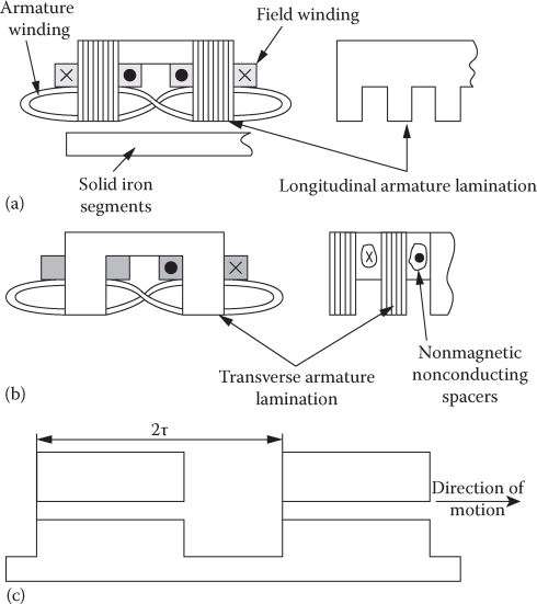
FIGURE 9.1 H-LSM layout (a) with longitudinal laminations primary core, (b) with transverse laminations, and (c) segmented and standard secondary solid care. (After Boldea, I. and Nasar, S.A., Linear Motion Electromagnetic Systems, John Wiley & Sons, New York, 1985.)

Images

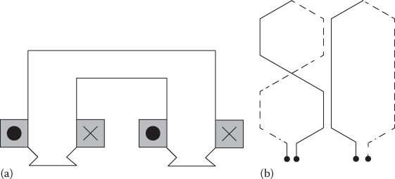
FIGURE 9.2 Armature coils: (a) segmented windings, (b) 8-shape (twisted) coils (c) straight coils. (After Boldea, I. and Nasar, S.A., Linear Motion Electromagnetic Systems, John Wiley & Sons, New York, 1985.)

Images

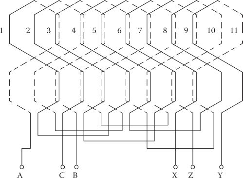
FIGURE 9.3 Typical q = 1 two-layer ac winding with 2/3 τ coil span with 8-shape coils (2p + 1 = 5-half-filled end poles as in LIMs). (After Boldea, I. and Nasar, S.A., Linear Motion Electromagnetic Systems, John Wiley & Sons, New York, 1985.)

Images

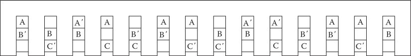
FIGURE 9.4 Three-layer ac winding (with short end connections) y/τ = 2/3, q = 1, 2p + 1 = 5).

9.2 DC Homopolar Excitation Airgap Flux Density and AC emf E₁

As the dc coils embrace the total H-LSM length, their airgap flux density pulsates with a period of 2τ but keeps the same polarity: opposite though below the two U core legs (Figure 9.5).

The secondary segment span (b_ps) varies around the pole pitch τ value; if larger levitation force is needed, τ_p = (1 ÷ 1.2)· τ, while when larger thrust is needed, τ_p=(0.7 ÷ 0.8)· τ; in the latter case, the normal (levitation) force is smaller. In general, to compromise between levitation and propulsion, τ_ps ≈ 1.0 × τ − g, where g = 10 ÷ 12 mm for urban (interurban) transportation and may go down to 1.0 ÷ 2.0 mm for industrial applications with a few meter long travels.

The calculation of the maximum airgap flux density, B₀_g, is rather straightforward:

B_{0 g} = \frac{μ_{0} \cdot W_{F} \cdot I_{F}}{2 g_{1} \cdot k_{C} (1 + k_{S})} (9.1)

$B_{0 g} = \frac{μ_{0} \cdot W_{F} \cdot I_{F}}{2 g_{1} \cdot k_{C} (1 + k_{S})} (9.1)$

where

W_FI_F is the field current mmf

g₁ is the airgap

k_C is the Carter coefficient:

k_{C} \approx \frac{1}{1 - γ \cdot \frac{b_{s l o t}}{τ_{s l o t}}}; γ \approx \frac{{(\frac{b_{s l o t}}{g_{1}})}^{2}}{5 + \frac{b_{s l o t}}{g_{1}}} (9.2)

$k_{C} \approx \frac{1}{1 - γ \cdot \frac{b_{s l o t}}{τ_{s l o t}}}; γ \approx \frac{{(\frac{b_{s l o t}}{g_{1}})}^{2}}{5 + \frac{b_{s l o t}}{g_{1}}} (9.2)$

Images

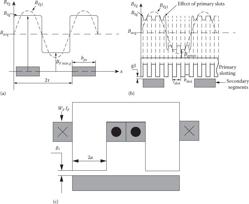
FIGURE 9.5 DC homopolar excitation airgap flux density: (a) ideal, (b) with primary slotting accounted for, and (c) transverse view.

k_S is the magnetic saturation coefficient; due to large airgap, even for heavy magnetic saturation, the value of k_S is expected to remain below 0.25. To obtain high normal and propulsion force densities, the value of B₀_g ≈ 1.3 ÷ 1.5 T. With an armature reaction flux density in the airgap of maximum 0.35 T, standard silicon U-shape transformer lamination cores may be used.

The minimum flux density in the airgap may be calculated using magnetic circuit method or FEM, but in general for g₁ = 10 mm, B_g_min ≈ (0.2 ÷ 0.24)B₀_g.

In a simpler calculation, a larger equivalent fictitious airgap g₂ may be used in between the track poles: g₂ ≈ 4· g, if τ/g > 10.

So the minimum airgap flux density B_F_min _g is

B_{F \min g} \approx \frac{g_{1}}{g_{2}} \cdot B_{0 g} \frac{1}{1 + k_{F r i n g e}} (9.3)

$B_{F \min g} \approx \frac{g_{1}}{g_{2}} \cdot B_{0 g} \frac{1}{1 + k_{F r i n g e}} (9.3)$

Using FEM, the more precise values of B₀_g and B_F_min _g may be found, and k_Fringe in (9.3) may be determined as a function of dc excitation mmf W_F · I_F for given machine geometry and airgap.

The airgap flux density fundamental B_Fg₁ is

B_{F g 1} \approx \frac{2}{π} \cdot (B_{a g} - B_{F \min g}) \cdot \sin (\frac{π}{2} \cdot \frac{τ_{p}}{τ}) (9.4)

$B_{F g 1} \approx \frac{2}{π} \cdot (B_{a g} - B_{F \min g}) \cdot \sin (\frac{π}{2} \cdot \frac{τ_{p}}{τ}) (9.4)$

In general, τ_p ≈ τ, as discussed before, for MAGLEVs; again, if only propulsion is needed, to minimize normal force, τ_p/τ ≈ 0.67 ÷ 0.7.

The emf per both ac winding legs is

E_{1} = π \cdot \sqrt{2} \cdot f_{1 r} \cdot ϕ_{p 1} \cdot k_{W_{1}} \cdot (2 W_{1}); ϕ_{p 1} = \frac{2}{π} B_{g 1} \cdot τ \cdot 2 a (9.5)

$E_{1} = π \cdot \sqrt{2} \cdot f_{1 r} \cdot ϕ_{p 1} \cdot k_{W_{1}} \cdot (2 W_{1}); ϕ_{p 1} = \frac{2}{π} B_{g 1} \cdot τ \cdot 2 a (9.5)$

where

E₁ is the phase RMS value of emf

W₁ is the turns per phase/primary leg

ϕ_p₁ is the ac flux/pole (peak value)

In (9.5), the two sides are connected in series (as for eight-shape-coil system); they may be connected in parallel also, to balance the normal force against track irregularities above the two U core legs alternatively; the two ac windings may be controlled by two 50% rating PWM inverters for more redundancy.

9.3 Armature Reaction and Magnetization Synchronous Inductances L_dm and L_qm

The three-phase ac winding produces, in turn, an armature reaction magnetic field in the airgap. Let us consider the ac traveling mmf J₁(x, t) as

J_{1} (x, t) = J_{1 m} \cdot \sin (\frac{π}{τ} x - ω_{1} t + δ_{i}) (9.6)

$J_{1} (x, t) = J_{1 m} \cdot \sin (\frac{π}{τ} x - ω_{1} t + δ_{i}) (9.6)$

where

J_{1 m} = \frac{3 \sqrt{2} \cdot k_{W_{1}} \cdot W_{1} \cdot I_{1}}{π \cdot p} (9.7)

$J_{1 m} = \frac{3 \sqrt{2} \cdot k_{W_{1}} \cdot W_{1} \cdot I_{1}}{π \cdot p} (9.7)$

and δ_i is the current power angle.

When in axis d, the armature reaction field “sees” the small airgap g₁ for the pole span and the large airgap g₂ in the interpole airgap zone; with transverse laminations, the magnetic field paths flow in the transverse plane and g₂ ≈ τ/π. Pure q axis current control is adequate for integrated suspension and propulsion control for decoupling the two functions; this situation is shown in Figure 9.6.

Based on the magnetic energy in the airgap W_md concept,

{(W_{m d})}_{δ_{i} = 0} = 3 X_{d m} \cdot I_{d}^{2}; {(W_{m q})}_{δ_{i} = \frac{π}{2}} = 3 X_{q m} \cdot I_{d}^{2} (9.8)

${(W_{m d})}_{δ_{i} = 0} = 3 X_{d m} \cdot I_{d}^{2}; {(W_{m q})}_{δ_{i} = \frac{π}{2}} = 3 X_{q m} \cdot I_{d}^{2} (9.8)$

with α = π · τ_p/τ, k = g₂/g₁:

X_{d m} \approx \frac{2}{π} [(\frac{α}{2} + \frac{1}{4} \sin 2 α) \cdot (1 - \frac{1}{k}) + \frac{π}{2 k}] X_{m} (9.9)

$X_{d m} \approx \frac{2}{π} [(\frac{α}{2} + \frac{1}{4} \sin 2 α) \cdot (1 - \frac{1}{k}) + \frac{π}{2 k}] X_{m} (9.9)$

X_{q m} \approx \frac{2}{π} [(\frac{α}{2} - \frac{1}{4} \sin 2 α) \cdot (1 - \frac{1}{k}) + \frac{π}{2 k}] X_{m} (9.10)

$X_{q m} \approx \frac{2}{π} [(\frac{α}{2} - \frac{1}{4} \sin 2 α) \cdot (1 - \frac{1}{k}) + \frac{π}{2 k}] X_{m} (9.10)$

Images

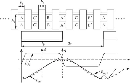
FIGURE 9.6 q axis reaction flux density.

where X_m is the magnetization inductance of the ac winding for smooth airgap (2g₁ · k_C) and including both U-shape leg ac coils in series (2W₁):

X_{m} = \frac{ω_{1} μ_{0} 6 {(2 W_{1} \cdot k_{W_{1}})}^{2} \cdot τ \cdot L}{2 g_{1} \cdot k_{C} \cdot (1 + k_{S}) \cdot p} (9.11)

$X_{m} = \frac{ω_{1} μ_{0} 6 {(2 W_{1} \cdot k_{W_{1}})}^{2} \cdot τ \cdot L}{2 g_{1} \cdot k_{C} \cdot (1 + k_{S}) \cdot p} (9.11)$

Again

2p is the poles of ac winding

k_C is the Carter coefficient

L = 2a is the width of one U core leg

The ac winding leakage reactance L_ls includes mainly the slot leakage and the end-connection leakage components. For “open slots” at both ends, the double-slot width (2b_S) is considered in the slot leakage inductance:

L_{l s} \approx 2 μ_{0} \frac{{(2 W_{1})}^{2}}{p_{1} \cdot q_{1}} (λ_{s} \cdot L + λ_{c} \cdot l_{l c}); X_{l s} = ω_{1} \cdot L_{l s} (9.12)

$L_{l s} \approx 2 μ_{0} \frac{{(2 W_{1})}^{2}}{p_{1} \cdot q_{1}} (λ_{s} \cdot L + λ_{c} \cdot l_{l c}); X_{l s} = ω_{1} \cdot L_{l s} (9.12)$

λ_{s} \approx \frac{h_{s}}{6 \cdot b_{s}}; λ_{c} \approx 0.66 \cdot q_{1}; l_{l c} \approx 2 \cdot τ (\frac{2}{3}) (9.13)

$λ_{s} \approx \frac{h_{s}}{6 \cdot b_{s}}; λ_{c} \approx 0.66 \cdot q_{1}; l_{l c} \approx 2 \cdot τ (\frac{2}{3}) (9.13)$

q₁ is the slots per pole per phase.

To complete the main parameter expressions, we add the ac winding resistance:

R_{s} = ρ_{c o} \cdot \frac{(2 W_{1}) \cdot j_{c o} \cdot W_{1} \cdot l_{c}}{(I_{1 n} \cdot W_{1})}; l_{c} = 2 L + 0.02 + l_{l c} (9.14)

$R_{s} = ρ_{c o} \cdot \frac{(2 W_{1}) \cdot j_{c o} \cdot W_{1} \cdot l_{c}}{(I_{1 n} \cdot W_{1})}; l_{c} = 2 L + 0.02 + l_{l c} (9.14)$

For the eight-shape coil in (9.14), 2W₁ becomes W₁, and l_c becomes 2l_c, where j_co is the rated (design) current density. The no-load steady-state voltage equation/phase is thus, as in a rotary synchronous machine,

{\underline{V}}_{S} = R_{S} {\underline{I}}_{S} + j X_{d} {\underline{I}}_{d} + j X_{q} {\underline{I}}_{q} - {\underline{E}}_{1} (9.15)

${\underline{V}}_{S} = R_{S} {\underline{I}}_{S} + j X_{d} {\underline{I}}_{d} + j X_{q} {\underline{I}}_{q} - {\underline{E}}_{1} (9.15)$

\begin{array}{l} {\underline{I}}_{S} = {\underline{I}}_{d} + {\underline{I}}_{q}; {\underline{E}}_{1} = - j X_{m a} {\underline{I}}_{F} \\ X_{d} = X_{l s} + X_{d m}; X_{q} = X_{l s} + X_{q m} \end{array} (9.16)

$\begin{array}{l} {\underline{I}}_{S} = {\underline{I}}_{d} + {\underline{I}}_{q}; {\underline{E}}_{1} = - j X_{m a} {\underline{I}}_{F} \\ X_{d} = X_{l s} + X_{d m}; X_{q} = X_{l s} + X_{q m} \end{array} (9.16)$

From (9.5), (9.1), and (9.3) and (9.4), the field armature coupling reactance X_ma is

X_{m a} \approx μ_{0} W_{1} \sqrt{2} k_{W_{1}} (2 W_{1}) W_{F} \cdot \frac{τ L}{k_{C} \cdot π^{2}} (\frac{1}{g_{1}} - \frac{1}{g_{2}}) \frac{1}{(1 + k_{S})} \sin \frac{π}{2} \frac{τ_{p}}{τ} (9.17)

$X_{m a} \approx μ_{0} W_{1} \sqrt{2} k_{W_{1}} (2 W_{1}) W_{F} \cdot \frac{τ L}{k_{C} \cdot π^{2}} (\frac{1}{g_{1}} - \frac{1}{g_{2}}) \frac{1}{(1 + k_{S})} \sin \frac{π}{2} \frac{τ_{p}}{τ} (9.17)$

Let us consider the general case of τ_p/τ ≠ 1 (X_dm ≠ X_qm or X_d ≠ X_q) and I_d ≠ 0 in the phasor diagram of Figure 9.7.

The electromagnetic power P_elm is, as in any SM,

P_{e l m} = 3 \cdot E_{1} \cdot I_{q} + 3 \cdot ω_{1} \cdot (L_{d} - L_{q}) \cdot I_{d} \cdot I_{q} = F_{x} \cdot 2 τ \cdot f_{1} (9.18)

$P_{e l m} = 3 \cdot E_{1} \cdot I_{q} + 3 \cdot ω_{1} \cdot (L_{d} - L_{q}) \cdot I_{d} \cdot I_{q} = F_{x} \cdot 2 τ \cdot f_{1} (9.18)$

Similarly the reactive power

Q_{1} = 3 \cdot E_{1} \cdot I_{d} + 3 \cdot (X_{d} \cdot I_{d}^{2} + X_{q} \cdot I_{q}^{2}) (9.19)

$Q_{1} = 3 \cdot E_{1} \cdot I_{d} + 3 \cdot (X_{d} \cdot I_{d}^{2} + X_{q} \cdot I_{q}^{2}) (9.19)$

Images

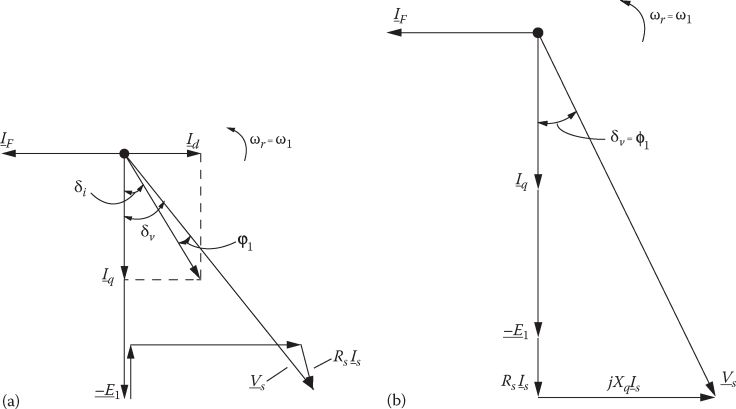
FIGURE 9.7 Phasor diagram of H-LSM with I_d ≠ 0, (a) and I_d = 0, (b).

F_{x} = (3 L_{m a} \cdot I_{F} \cdot I_{q} + 3 (L_{d} - L_{q}) \cdot I_{d} \cdot I_{q}) \cdot \frac{π}{τ} (9.20)

$F_{x} = (3 L_{m a} \cdot I_{F} \cdot I_{q} + 3 (L_{d} - L_{q}) \cdot I_{d} \cdot I_{q}) \cdot \frac{π}{τ} (9.20)$

Note: I_d, I_q are phase variables (RMS values of them).

The total magnetic energy in the machine W_mt when neglecting magnetic saturation is

W_{m t} \approx \frac{Q_{1}}{ω_{1}} (9.21)

$W_{m t} \approx \frac{Q_{1}}{ω_{1}} (9.21)$

and the normal (attraction) force F_n is

F_{n} = \frac{\partial W_{m t}}{\partial g_{1}} \approx - \frac{W_{m t}}{g_{1}} (9.22)

$F_{n} = \frac{\partial W_{m t}}{\partial g_{1}} \approx - \frac{W_{m t}}{g_{1}} (9.22)$

Thus, from the phasor diagram, I_d and I_q are

\begin{array}{l} I_{d} = \frac{(E_{1} - V_{S} \cdot \cos δ_{V}) \cdot X_{q} + R_{S} \cdot V_{S} \sin δ_{V}}{R_{S}^{2} + X_{d} \cdot X_{q}} \\ I_{q} = \frac{V_{S} \cdot (R_{S} \cdot \cos δ_{V} + X_{d} \cdot \sin δ_{V}) - R_{S} \cdot E_{1}}{R_{S}^{2} + X_{d} \cdot X_{q}} \end{array} (9.23)

$\begin{array}{l} I_{d} = \frac{(E_{1} - V_{S} \cdot \cos δ_{V}) \cdot X_{q} + R_{S} \cdot V_{S} \sin δ_{V}}{R_{S}^{2} + X_{d} \cdot X_{q}} \\ I_{q} = \frac{V_{S} \cdot (R_{S} \cdot \cos δ_{V} + X_{d} \cdot \sin δ_{V}) - R_{S} \cdot E_{1}}{R_{S}^{2} + X_{d} \cdot X_{q}} \end{array} (9.23)$

Finally, the power factor cos φ and efficiency η are

\cos φ = \frac{F_{X} \cdot 2 τ f_{1} + 3 \cdot R_{S} \cdot I_{S}^{2}}{3 \cdot V_{S} I_{S}}; η \approx \frac{1}{1 + \frac{3 \cdot R_{S} I_{S}^{2}}{F_{X} \cdot 2 τ \cdot f_{1}}}; I_{S}^{2} = I_{d}^{2} + I_{q}^{2} (9.24)

$\cos φ = \frac{F_{X} \cdot 2 τ f_{1} + 3 \cdot R_{S} \cdot I_{S}^{2}}{3 \cdot V_{S} I_{S}}; η \approx \frac{1}{1 + \frac{3 \cdot R_{S} I_{S}^{2}}{F_{X} \cdot 2 τ \cdot f_{1}}}; I_{S}^{2} = I_{d}^{2} + I_{q}^{2} (9.24)$

Example 9.1

For the so far developed preliminary theory, let us consider the following data: U_s = 90 m/s, 2p = 12 poles, τ = 0.45 m, L = 2a = 0.25 m, g₁ = 0.02 m (!), W₁ = 305 turns per phase, k_W₁ = 1 (winding factor, say, q₁ = 1, y/τ = 1), W_FI_F = 30,000 A turns, V_S = 3 kV(RMS value); τ_p/τ ≈ 1. It is required to calculate F_x_′ F_y_′ (F_n), η, cos φ versus power angle δ (δ_V).

Solution

Applying Equations 9.1 through 9.24, we get the results in Figure 9.8:

The results in Figure 9.8 warrant remarks such as the following:

For I_d = 0, which corresponds to δ_v ≈ 45°, sizeable rated thrust, normal force, and good power factor (cos φ > 0.8) and efficiency (η > 0.95) are obtained.
The dc winding copper (or aluminum) losses are not considered here but, even if they would, the losses would be up to 10% of rated power; the total efficiency would be then above 85%; but it will provide for both suspension and propulsion in MAGLEV applications.
The normal force to thrust ratio for δ_v = 45° is more than 12/1, which means that more thrust is available, if the maximum vehicle acceleration is limited to 1 m/s² with the H-LSM making 10% of vehicle total weight. When fully loaded with people or freight, the normal force to thrust will be around 10/1.
The earlier example is rather general, and no attempt at optimal design was made; the pole pitch τ = 0.45 m is rather high; 0.2 ÷ 0.25 m would be more adequate, as the U-shape core legs width L = 2a ≈ 0.2 ÷ 0.25 m, to reduce the track segments weight (and cost).
The maximum dc produced airgap flux density B₀_g could go as high as 1.6 T, for high saturation flux density, and, with an airgap g₁ = 10 mm, outstanding performance is to be expected, for integrated propulsion and suspension functions on MAGLEVs.

Images

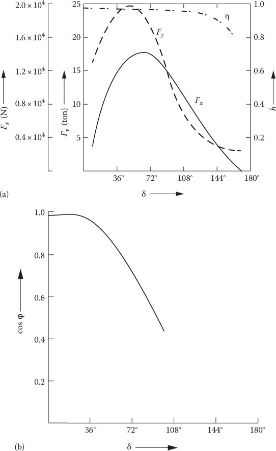
FIGURE 9.8 H-LSM steady-state characteristics: (a) thrust F_x, normal force F_y (F_n) and efficiency, (b) power factor. (After Boldea, I. and Nasar, S.A., Linear Motion Electric Machine, John Wiley & Sons, New York, 1976.)

9.4 Longitudinal end Effect in H-LSM

The dc field winding and the primary core have a limited length along the direction of motion; the latter moves at speed U_s with respect to the solid-iron secondary (track) segments (Figure 9.9).

These induced eddy currents in a secondary segment at its entry into the primary will decay in time, while the segment “travels” along the primary length; a similar effect occurs at a secondary segment exit from primary.

The eddy currents thus created manifest themselves in a drag force F_d, a reduction of normal force, and by additional losses (lower efficiency). These eddy current influences on performance are called the longitudinal end effect. As in Ref. [8], through a rather complete theory, it was demonstrated that the longitudinal end effect even at 100 m/s has a thrust and normal force reduction effect of less than 10%–15% (with similar effects on losses). We may treat here the longitudinal end effect by a simplified model, easier to use in optimization design. This is in sharp contrast to LIMs, where dynamic longitudinal effects at high speeds are much higher.

The main assumptions are the following:

The current induced in the secondary segments exhibits only a transverse (J_y) component (Figure 9.9); the inevitable presence of longitudinal component (J_x) is accounted for by the Russel-Northworthy coefficient (see the chapters on LIMs) k_t:

$k_{t} \approx \frac{1}{[1 - \frac{\tanh β a_{e}}{β a_{e} \cdot (1 + \tanh β a_{e} \cdot \tanh β (c - a_{e}))}]} (9.25)$ $k_{t} \approx \frac{1}{[1 - \frac{\tanh β a_{e}}{β a_{e} \cdot (1 + \tanh β a_{e} \cdot \tanh β (c - a_{e}))}]} (9.25)$

with

$a_{e} \approx \frac{L}{2} + g_{1}; c \approx \frac{L_{W}}{4} + a; β = \frac{π}{τ_{p}} (9.26)$ $a_{e} \approx \frac{L}{2} + g_{1}; c \approx \frac{L_{W}}{4} + a; β = \frac{π}{τ_{p}} (9.26)$

where L_w is the window area width between the primary U core legs; the approximation for c takes into account the single secondary segment with two primary U core leg interaction in defining the eddy current density lines:
The magnetic field is zero outside the primary core.
The induced current distribution along O_x (direction of motion) is uniform inside and outside the core.
The secondary segment magnetic permeability is constant but it is iteratively calculated.
The depth of field penetration in the secondary segment is also iteratively calculated [9].
The reaction field of induced currents is neglected.
The eddy currents in the entry and exit secondary segments die out quickly and thus only their influence on longitudinal end effect is considered here (see Ref. [8] for a more detailed analysis).

Images

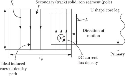
FIGURE 9.9 Ideal secondary induced currents at H-LSM primary entry.

Consequently, with ψ_F as dc field current flux in the entry segment, speed U, and segment resistance R, we have

- \frac{d ψ_{F}}{d t} = \frac{d ψ_{F}}{d t} \cdot U = R \cdot I (9.27)

$- \frac{d ψ_{F}}{d t} = \frac{d ψ_{F}}{d t} \cdot U = R \cdot I (9.27)$

R = \frac{2 k_{t} a_{e}}{σ_{i} \cdot d i} (\frac{1}{x} + \frac{1}{τ_{p} - x}) (9.28)

$R = \frac{2 k_{t} a_{e}}{σ_{i} \cdot d i} (\frac{1}{x} + \frac{1}{τ_{p} - x}) (9.28)$

Approximately

\frac{d ψ_{F}}{d x} = 2 B_{0 g} a_{e} (9.29)

$\frac{d ψ_{F}}{d x} = 2 B_{0 g} a_{e} (9.29)$

with B₀_g from (9.1).

The effect of armature traveling field on longitudinal end effect is neglected here. From the previous equations, the current I in the secondary segment is (Figure 9.9)

I = \frac{U \cdot B_{0 g}}{\frac{μ_{0} U}{2 g_{0}} + \frac{k_{t} \cdot τ_{p}}{d_{i} \cdot σ_{i} x (τ_{p} - x)}} (9.30)

$I = \frac{U \cdot B_{0 g}}{\frac{μ_{0} U}{2 g_{0}} + \frac{k_{t} \cdot τ_{p}}{d_{i} \cdot σ_{i} x (τ_{p} - x)}} (9.30)$

where σ_i is the iron electrical conductivity.

The drag force, for both U core legs and entry segment F_d, is

F_{d} = I \cdot B_{0 g} 4 a_{e} = \frac{4 U \cdot B_{0 g}^{2} a_{e}}{\frac{μ_{0} U}{2 g_{0}} + \frac{k_{t} \cdot τ_{p}}{d_{i} \cdot σ_{i} x (τ_{p} - x)}} (9.31)

$F_{d} = I \cdot B_{0 g} 4 a_{e} = \frac{4 U \cdot B_{0 g}^{2} a_{e}}{\frac{μ_{0} U}{2 g_{0}} + \frac{k_{t} \cdot τ_{p}}{d_{i} \cdot σ_{i} x (τ_{p} - x)}} (9.31)$

The maximum drag force F_d_max occurs at x = τ_p/2. The average drag force (considering both entry and exit segments, with 2p poles per primary) is F_d ≈ F_d _max:

F_{d a v} = F_{d \max} \approx \frac{4 U \cdot B_{0 g}^{2} a_{e}}{\frac{μ_{0} U}{2 g} + \frac{k_{t} \cdot U}{d i \cdot σ_{i} τ_{p}}} (9.32)

$F_{d a v} = F_{d \max} \approx \frac{4 U \cdot B_{0 g}^{2} a_{e}}{\frac{μ_{0} U}{2 g} + \frac{k_{t} \cdot U}{d i \cdot σ_{i} τ_{p}}} (9.32)$

Note: As the reaction of the eddy currents I has been neglected, their influence on normal force is also neglected. Ref. [8] includes the reduction of normal force due to longitudinal end effect.

Experimental results (Ref. [8]) confirm the theory, for a 30 m/s max speed test platform (Figure 9.10) in relation to normal force reduction and drag force increase with speed (2pτ = 0.62 m, 2a = 0.03 m, τ_p = 0.069 m = τ, g₁k_C = 6.7 mm).

Images

FIGURE 9.10 Average drag (F_x) and total average normal force F_n versus speed for an H-LSM (longitudinal end effect). (After Boldea, I. and Nasar, S.A., EME J. (now EPCS), Taylor & Francis, 2(2), 254, 1978.)

It is estimated that for a 1 MW H-LSM with a total stack width (2 × 2a = 0.15 m), 2.5 m long at 100 m/s, the drag force power (F_x_av U)-longitudinal effect losses are less than 65 kW. This is quite acceptable and proves the suitability of the H-LSM for high-speed MAGLEVs with solid mild steel track segments. The normal force decrease with speed due to longitudinal end effect at 100 m/s is less than 15%, to prove once more this claim.

9.5 Preliminary Design Methodology by Example

The design methodology starts with preliminary specifications such as

Rated (or peak) thrust: F_xu = 6 kN (8 H-LSMs for a 36 ton MAGLEV)
Rated normal force F_n = 4.5 ton
Rated (peak) speed U_n = 100 m/s
Rated ac phase voltage (maximum RMS value): V_S = 1080 V

Pure I_q control

Rated (and boost) dc voltage for field winding supply: not given here.

Besides this data, quite a few parameters are given from prior experience, such as the following:

Airgap g₁ = 1.5 × 10⁻² m (from mechanical reasons, it could be lowered to g₁ = 1.0 × 10⁻² m).
Secondary track segments total width L_s < 0.35 m (L_s = 2 × 2a + L_W); this limitation should keep the track cost within reasonable bounds.
Maximum H-LSM length: 2pτ < 3.7 m (to accept tight curves).

With this data in mind, we return to a few important items that provide the mathematics for the preliminary design. Then we use the case study data to produce sample design results.

9.5.1 Armature AC Winding Specifics and Phasor Diagram

The two practical ac windings of interest have been already introduced in Section 9.1. The eight-shape-coil ac winding (Figure 9.11) seems the first choice, especially with three slots/pole (q = 1 slot/pole/phase) and diametrical coils (y/τ = 1) to yield unity fundamental winding factor $k_{w_{1}}$ $k_{w_{1}}$ .

Images

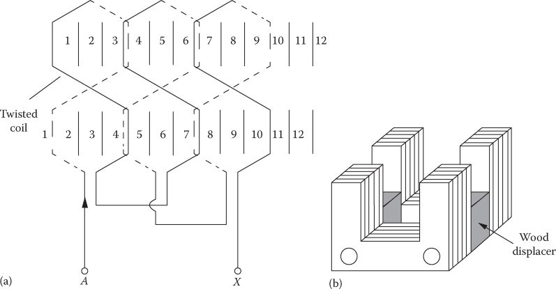
FIGURE 9.11 Eight-shape ac coil winding for H-LSM (a), transverse (U shape) primary cores, (b). (After Boldea, I. and Nasar, S.A., EME J. (now EPCS), Taylor & Francis, 4(2–3), 125, 1979.)

The three-layer winding (Figure 9.4) has its own merits in reducing the end connections of coils (mainly for 2a ≤ τ) and in providing space for airflow between layers, but its fundamental winding factor is only 0.867.

For transverse (transformer) lamination primary cores, the armature reaction field is also transverse (ac coil slots are open at both ends), and thus, the interaction between propulsion and suspension functions for pure I_q control (Figure 9.11) is notably reduced.

The phasor diagram in Figure 9.7b stands for MAGLEVs, L_d = L_q = L_s (τ_p/τ ≈ 1), to provide enough normal force.

Note: When small normal force design is required, either the ratio τ_p/τ is reduced to 0.65–0.7 or a double-sided structure is used. At the limit when short travel of primary on linear bearings is adopted, the dc coils may be replaced by primary long PMs [14] (Figure 9.12).

Again, to reduce the radial force on each U core, τ_p/τ = 0.65–0.70, after optimization attempts.

Images

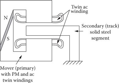
FIGURE 9.12 Ideally zero normal force H-LSM with concentrated flux PM homopolar excitation. (From Evers, W. et al., Record of LDIA-1998, Tokyo, Japan, pp. 46–49, 1998.)

Images

FIGURE 9.13 Transverse leakage flux lines of dc excitation coils.

9.5.2 Primary Core Teeth Saturation Limit

With pure I_q control (typical with PWM voltage-source inverters), in MAGLEVs (Figure 9.6), the teeth on the second half of the pole pitch experience both the dc excitation and full ac magnetic flux density B₀_g (9.1).

The armature reaction airgap flux density translates into a larger teeth flux density. So its influence should be enlarged by the slot pitch/tooth length ratio: on top of that, the leakage flux density $B_{w_{1}}$ $B_{w_{1}}$ in the U core window has to be added as it is notable (Figure 9.13).

We may not add flux densities unless magnetic saturation is ignored (or kept constant (known)). So the total maximum primary tooth flux density B_t_max is approximately

B_{t \max} \approx [\frac{μ_{0} W_{F} I_{F}}{k_{C}} (\frac{1}{2 g_{1}} + \frac{h_{s}}{τ \cdot L_{W}}) + \frac{τ_{s}}{b_{t}} \cdot \frac{3 \sqrt{2} (2 W_{1}) I_{1} k_{w 1}}{p (2 g_{1}) k_{C}}] \frac{1}{1 + k_{s} (B_{t \max})} (9.33)

$B_{t \max} \approx [\frac{μ_{0} W_{F} I_{F}}{k_{C}} (\frac{1}{2 g_{1}} + \frac{h_{s}}{τ \cdot L_{W}}) + \frac{τ_{s}}{b_{t}} \cdot \frac{3 \sqrt{2} (2 W_{1}) I_{1} k_{w 1}}{p (2 g_{1}) k_{C}}] \frac{1}{1 + k_{s} (B_{t \max})} (9.33)$

where

τ_s is the tooth pitch

b_t is the tooth span

Equation 9.33 unveils an iterative process, as heavy magnetic saturation with B_t_max = 1.85 ÷ 1.9 T (even 2.2 T for special, high-saturation flux density, silicon lamination) is practical. B_t_max is a design parameter as it limits how low L_W could go, together with the constraint of enough room for ac end coils.

9.5.3 Preliminary Design Expressions

With L_S limited to 0.3−0.35 m, we may infer that

L_{S} \approx 4 a + \frac{τ \cdot c_{1}}{\sqrt{3}} + 0.03 < 0.3 \div 0.35 m (9.34)

$L_{S} \approx 4 a + \frac{τ \cdot c_{1}}{\sqrt{3}} + 0.03 < 0.3 \div 0.35 m (9.34)$

Also 2p • τ < 3.7 m; c₁ ≥ 1. To quickly calculate the pole pitch τ, the thrust and normal force expressions are recalculated here:

F_{x n} = \frac{3 E_{1} I_{1} (1 - \frac{F_{d}}{F_{x n}})}{2 τ f}; \frac{F_{d}}{F_{x n}} \approx 0.05 \div 0.1 (9.35)

$F_{x n} = \frac{3 E_{1} I_{1} (1 - \frac{F_{d}}{F_{x n}})}{2 τ f}; \frac{F_{d}}{F_{x n}} \approx 0.05 \div 0.1 (9.35)$

F_{n} \approx \frac{B_{0 g}^{2} \cdot 2 a \cdot 2 p τ}{2 μ_{0}}; (I_{q} control) (9.36)

$F_{n} \approx \frac{B_{0 g}^{2} \cdot 2 a \cdot 2 p τ}{2 μ_{0}}; (I_{q} control) (9.36)$

where F_d is the longitudinal effect (braking) force (9.31).

With a large airgap (g₁ = 1.5 × 10⁻² m), the airgap flux density of dc coils B₀_g ≈ 0.85 T (much larger values (1.5−1.6 T) could be adopted for superior laminations with B_sat = 2.35 T!), to limit the U core window weight. The U core leg width (2a) can now be calculated, by fixing 2pτ (primary length), from (9.35), with given normal force F_n.

Then, from (9.34), the pole pitch τ is obtained. The number of Ampere turns per winding (2W₁I₁) follows then from (9.35) for given thrust F_xa. From here on the slot height h_S, calculation for given τ and q₁ = 1 is straightforward.

And so all parameters and performance based on technical theory developed in previous paragraphs may be calculated.

Typical results for our numerical example are as follows:

j_F = 15 A/mm²—rated current density in the field coils (forced cooling)

j_Co = 20 A/mm²—rated current density in ac windings (forced cooling)

τ = 0.18 m—pole pitch

2p = 20—number of poles

L_W = 0.158 m—window width

2a = 7.08 × 10⁻² m—U core one leg width

f_n = 274 Hz—rated frequency

In ≈ 250 A

W₁ ≈ 114 turns/phase

VS ≈ 1080 V

cos φ₁ = 0.8368

W_FI_F ≈ 22,332 A turns—field coils mmf

F_d ≈ 280 N (longitudinal effect drag force at d_i = 0.6 × 10−3 m)

η₁ ≈ 0.95—efficiency without dc winding losses

η_net = 0.836—total efficiency (with dc winding losses)

F_xn = 6 kN—total thrust

F_n = 4.5 ton—normal force

T_F = 0.04 s—dc field circuit time constant

p_exc = 65 kW—dc field coil losses

h_s = 0.09 m—ac coil slot height

The preliminary design may be discussed as follows:

As the dc current produced airgap flux density B₀_g is only B₀_g = 0.85 T, the ratio of 7.5/1 of normal force/thrust is obtained at an airgap g₁ = 1.5 × 10⁻² m. A smaller airgap (g₁ = 1 × 10⁻² m) with B₀_g = 1.3−1.5 T (for high saturation flux density laminations) would allow notably better performance; still the preliminary design yields acceptable performance for integrated propulsion suspension of a MAGLEV at 100 m/s, such as 0.886 kg/kW for the H-LSM at η_net = 0.836 and cos φ=0.8368.
The previous preliminary design should be used only as a starting point; FEM analysis is to be performed to calculate B_g_min and thus more precisely B_g₁ (fundamental airgap flux density in the airgap produced only by the dc winding); B_g₁ is crucial for thrust force computation F_xn.
A more detailed analytical model with 2 (3) D FEM correction factors may be used for an optimization design methodology; finally, again, key 2 (3) D FEM should be used to validate the optimal analytical design.
An example of an H- LSM as applied to an urban MAGLEV 4 ton research prototype (Magnibus-01) will be presented in more detail in a later chapter on “Passive Guideway MAGLEVs” [16].
The application of H-LSM with PM excitation [14] for short travel (a few meters) on linear bearings or on wheels, though interesting in nature, is not pursued here.
The H- LSM with 1.3–1.5 T dc airgap flux density leads to overall propulsion and suspension performance, which makes the latter very performance/cost competitive for MAGLEVs, where its large normal force is fully exploited.

9.6 H-LSM Model for Transients and Control

H-LSM behaves like a rotary synchronous machine with dc excitation, L_d = L_q = L_s (only in MAGLEVs), and with a very weak damper cage represented by the solid-iron secondary segments. For simplicity, we neglect this cage effect.

It should also be noticed that there are basically two sets of equations of motion: vertical (suspension) and longitudinal (propulsion) motion. The drag force, F_d = k_d · U, acts as a damper for the propulsion motion longitudinal oscillations.

We may now simply write the dq model of H-LSM in stator coordinates:

\begin{array}{l} {\bar{V}}_{S} = R_{S} {\bar{I}}_{S} + \frac{d {\bar{ψ}}_{S}}{d t} - j ω_{r} {\bar{Ψ}}_{S}; ω_{r} = \frac{π}{τ} U; {\bar{V}}_{S} = V_{d} + j V_{q}; {\bar{I}}_{S} = I_{d} + j I_{q} \\ {\bar{ψ}}_{S} = L_{S l} I_{d} + L_{d m} (g_{1}) (I_{d} + I_{F}^{p}) + j (L_{S l} I_{q} + L_{q m} (g_{1}) I_{q}) \\ I_{F}^{p} = k_{I_{F}} \cdot I_{F}; k_{I_{F}} = {(\frac{L_{d m}}{M_{a F}})}^{- 1}; I_{F}^{p} is the field current reduced to primary \\ I_{F} R_{F} - V_{F} = - L_{F l} \frac{d I_{F}}{d t} - \frac{d L_{d m} (g_{1})}{d t} (k_{I_{F}} \cdot I_{F} + I_{d}) \cdot k_{I_{F}} \\ m \frac{d u}{d t} = F_{x} - F_{L o a d} - F_{d}; F_{x} = \frac{3}{2} \frac{π}{τ} Real (j {\bar{ψ}}_{S} \cdot {\bar{I}}_{S}^{*}); F_{d} \approx {k^{'}}_{d} \cdot {(\frac{I_{F}}{g_{1}})}^{2} \cdot U \\ or F_{x} = \frac{3}{2} \frac{π}{τ} [L_{d m} (g_{1}) I_{F}^{p} + (L_{d m} (g_{1}) - L_{q m} (g_{1})) I_{d}] \cdot I_{q} \\ m \frac{d U_{V}}{d t} = m \cdot g - F_{n}; F_{n} \approx \frac{2 a .2 p τ}{2 □_{0}} \cdot {(\frac{□_{0} W_{F} I_{F}}{2 g_{1} k_{C} (1 + k_{S})})}^{2}; \frac{d g_{1}}{d t} = U_{V} \end{array} (9.37)

$\begin{array}{l} {\bar{V}}_{S} = R_{S} {\bar{I}}_{S} + \frac{d {\bar{ψ}}_{S}}{d t} - j ω_{r} {\bar{Ψ}}_{S}; ω_{r} = \frac{π}{τ} U; {\bar{V}}_{S} = V_{d} + j V_{q}; {\bar{I}}_{S} = I_{d} + j I_{q} \\ {\bar{ψ}}_{S} = L_{S l} I_{d} + L_{d m} (g_{1}) (I_{d} + I_{F}^{p}) + j (L_{S l} I_{q} + L_{q m} (g_{1}) I_{q}) \\ I_{F}^{p} = k_{I_{F}} \cdot I_{F}; k_{I_{F}} = {(\frac{L_{d m}}{M_{a F}})}^{- 1}; I_{F}^{p} is the field current reduced to primary \\ I_{F} R_{F} - V_{F} = - L_{F l} \frac{d I_{F}}{d t} - \frac{d L_{d m} (g_{1})}{d t} (k_{I_{F}} \cdot I_{F} + I_{d}) \cdot k_{I_{F}} \\ m \frac{d u}{d t} = F_{x} - F_{L o a d} - F_{d}; F_{x} = \frac{3}{2} \frac{π}{τ} Real (j {\bar{ψ}}_{S} \cdot {\bar{I}}_{S}^{*}); F_{d} \approx {k^{'}}_{d} \cdot {(\frac{I_{F}}{g_{1}})}^{2} \cdot U \\ or F_{x} = \frac{3}{2} \frac{π}{τ} [L_{d m} (g_{1}) I_{F}^{p} + (L_{d m} (g_{1}) - L_{q m} (g_{1})) I_{d}] \cdot I_{q} \\ m \frac{d U_{V}}{d t} = m \cdot g - F_{n}; F_{n} \approx \frac{2 a .2 p τ}{2 □_{0}} \cdot {(\frac{□_{0} W_{F} I_{F}}{2 g_{1} k_{C} (1 + k_{S})})}^{2}; \frac{d g_{1}}{d t} = U_{V} \end{array} (9.37)$

No track irregularities are yet considered previously. We should add the Park transformation:

| \begin{matrix} I_{d} \\ I_{q} \\ I_{0} \end{matrix} | = \frac{2}{3} | \begin{matrix} \cos (- θ_{e r}) & \cos (- θ_{e r} + \frac{2 π}{3}) & \cos (- θ_{e r} - \frac{2 π}{3}) \\ \sin (- θ_{e r}) & \sin (- θ_{e r} + \frac{2 π}{3}) & \sin (- θ_{e r} - \frac{2 π}{3}) \\ \frac{1}{2} & \frac{1}{2} & \frac{1}{2} \end{matrix} | | \begin{matrix} I_{a} \\ I_{b} \\ I_{c} \end{matrix} | (9.38)

$| \begin{matrix} I_{d} \\ I_{q} \\ I_{0} \end{matrix} | = \frac{2}{3} | \begin{matrix} \cos (- θ_{e r}) & \cos (- θ_{e r} + \frac{2 π}{3}) & \cos (- θ_{e r} - \frac{2 π}{3}) \\ \sin (- θ_{e r}) & \sin (- θ_{e r} + \frac{2 π}{3}) & \sin (- θ_{e r} - \frac{2 π}{3}) \\ \frac{1}{2} & \frac{1}{2} & \frac{1}{2} \end{matrix} | | \begin{matrix} I_{a} \\ I_{b} \\ I_{c} \end{matrix} | (9.38)$

Images

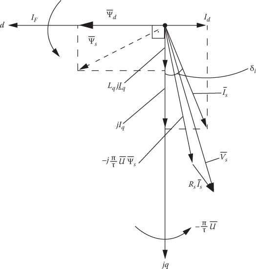
FIGURE 9.14 The vector (space phasor) diagram of H-LSM (steady state, I_d ≠ 0).

The sign (−) for θ_er in (9.39) stems from the fact that the primary is moving against its traveling field (Figure 9.14):

\frac{d θ_{e r}}{d t} = - \frac{π}{τ} u + \frac{π}{2} + δ_{i} (9.39)

$\frac{d θ_{e r}}{d t} = - \frac{π}{τ} u + \frac{π}{2} + δ_{i} (9.39)$

As expected, Figures 9.7 and 9.14 are very similar in terms of angles, but it is time angles in Figure 9.7 and space angles in Figure 9.14 as the latter deals with space vectors and not with phase variables.

The same Park transformation is valid for the voltage vectors. Once the voltages V_a, _b, _c(t), F_load, k_d′, V_F(t), and H-LSM parameters are given, numerical methods allow investigating any transients by (9.36) through (9.38).

For given airgap, the vertical equations of motion are eliminated and the order of the system degenerates from 7th (I_d, I_q, I_F, U, θ_er, U_v, to 5th (I_d, I_q, I_F, U, θ_er). The propulsion and the suspension close-loop control add more equations (and orders) to this system of equations.

A generic structural diagram for Equation 9.37 for constant airgap, pure propulsion control, is given in Figure 9.15.

Note: In Figure 9.15, the V_F and I_F are actual field winding input voltage and current.

As noticed in Figure 9.15, there are only two leakage electric time constants to consider, in the absence of the secondary damping cage (see Ref. [13] for an SM with damper cage).

Magnetic saturation occurs in ψ_dm and ψ_qm. The airgap variation also marks its presence in ψ_dm

Images

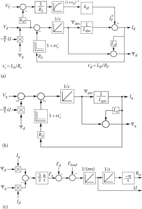
FIGURE 9.15 Generic structural diagrams of H-LSM: (a) axis d, (b) axis q, and (c) motion equations (constant airgap, g₁).

9.7 Vector Thrust (Propulsion) and Flux (Suspension) Control

Based on the circuit model, a recently developed generic vector control system of H-LSM is shown in Figure 9.16.

The rather complex control in Figure 9.16 may be somewhat clarified by remarks such as the following:

zero $I_{d}^{*}$ $I_{d}^{*}$ vector control is chosen to reduce propulsion-suspension interaction (in practice, it is not zero but it is small).
PI + SM (sliding mode) control for airgap, speed, and current controllers is chosen to provide robust control in the presence of airgap and magnetic saturation (inductance) variations.
In the presence of a secondary mechanical suspension system for each H-LSM on a MAGLEV, rather independent but highly robust, partly decentralized, airgap control is feasible.
For propulsion-only control, the reference field current may be made dependent either on reference thrust $F_{d}^{*}$ $F_{d}^{*}$ (to minimize total copper losses, for example) or it is kept constant up to base speed and then decreased with speed for constant power wide-speed range.
Either mover position (with respect to secondary (track) segments) or mover speed may be measured or estimated, for motion sensorless control; for nonhesitant start, initial mover position has to be known (or estimated).
The emf compensation network improves performance at high speeds by relaxing somewhat the contribution of PI + SM I_d, I_q current controllers.

Images

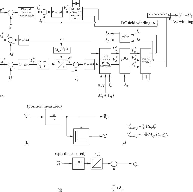
FIGURE 9.16 Vector control of H-LSM (integrated propulsion and suspension control): (a) vector control, (b) position angle and speed from measured position, (c) emf decoupling network, and (d) position angle θ_er from measured speed.

Typical vector control results for a four H-LSM (in parallel) MAGLEV (MAGNIBUS-01) are given in Ref. [16].

While, in the 1980s, current source inverters were used for the H- LSM control [6,17], today PWM voltage-source inverters, one for each H-LSM control, provide higher efficiency and lower converter weight in integrated vector MAGLEV propulsion and suspension control.

9.8 Summary

Homopolar linear synchronous motors (H-LSM) are characterized by a solid mild steel track with magnetic anisotropy and a transverse multiple U-shape primary silicon lamination mover (primary) provided with a primary long dc coil for excitation and a three-phase ac winding.
The primary long dc coil currents produce a homopolar, pulsating, airgap flux density with 2p poles; the fundamental of this flux density is aligned to the secondary segments axis (axis d) and interacts with the ac winding mmf to produce thrust (F_x).
The resultant airgap flux density produces a normal (attraction) force, which may be used for controlled magnetic levitation (suspension) of the vehicle (F_n).
Ratios of F_n/F_x ≥ 10/1 may be obtained with rather undecoupled control of suspension and propulsion, if pure I_q control for propulsion is accompanied by field current control for levitation.
When levitation control is not needed, double -sided primaries may be used “to sandwich” the segmented (variable anisotropy) secondary (track), for ideally zero vertical force between primary and secondary; to reduce the vertical force between the two sides of the primary, the secondary segment span is reduced to τ_p/τ = 0.6 ÷ 0.7.
For dc field current flux density of 1.3 ÷ 1.5 T, rather good integrated propulsion-suspension performance can be obtained in terms of efficiency, power factor, and in terms of thrust and normal force per weight.
It has been shown that the eddy currents induced in the solid iron segments due to their motion for limited primary length, that is the longitudinal end effect, have mild (10%) influences on thrust, normal force, and on efficiency, even at 100 m/s speed.
Preliminary design examples indicate total efficiency above 85% (for integrated propulsion and suspension) and power factor above 80% for up to 100 m/s MAGLEVs, but 2 (3) D FEM should be used to calculate more precisely the performance.
The dq model of H-LSM contains inductances L_dm, L_qm, which depend on airgap; in general, the airgap varies due to track irregularities or during levitation control. This makes the dq model of H-LSM highly nonlinear, besides the influence of the product of variables and magnetic saturation.
Very robust vector control [18] of H-LSM for decoupled propulsion and levitation control is required to account for these nonlinearities.
Passive guideway H-LSM MAGLEVs, for urban and interurban transportation, should be investigated aggressively now that high-performance PWM inverters and mechanical electric power collection (through controlled pantographs) in the MW power range are available up to 120 m/s and more.

References

1. E. Rummich, Linear synchronous machines—Theory and construction, Bull. ASE, 23, 1972, 1338–1344 (in French).

2. M. Guarino, Jr., Integrated linear electric motor propulsion system for high speed transportation, Record of International Symposium on Linear Electric Motors, Lyon, France, 1974.

3. E. Levi, Preliminary design studies of iron core synchronous operating linear motor, Polytechnical & Institute of Brooklyn, Report no. 76/005, 1976, DOT ORD, Washington, DC.

4. I. Boldea and S.A. Nasar, Linear Motion Electric Machine, Chapter 9, John Wiley & Sons, New York, 1976.

5. H. Lorenzen and W. Wild, The Synchronous linear motor, Intern Report, Technical University of Munich, 1976 (in German).

6. B.T. Ooi, Homopolar linear synchronous motor, Record of ICEM-1979, Brussels, Belgium.

7. T.R. Haden and W.R. Mischler, A comparison of linear induction and synchronous homopolar motors, IEEE Trans., MAG-14(5), 1978, 924–926.

8. I. Boldea and S.A. Nasar, Field winding drag and normal forces in linear synchronous homopolar motors, EME J. (now EPCS), Taylor & Francis, 2(2), 1978, 254–268.

9. I. Boldea and S.A. Nasar, Linear synchronous homopolar motor—Design procedure for propulsion and levitation, EME J. (now EPCS), Taylor & Francis, 4(2–3), 1979, 125–136.

10. I. Boldea and S.A. Nasar, Thrust and normal force pulsations of current inverter—Fed linear induction motors, EME J. (IBID), 7(2), 1982.

11. G.R. Slemon, A homopolar linear synchronous motor, Record of ICEM-1979, Brussels, Belgium.

12. I. Boldea and S.A. Nasar, Linear Motion Electromagnetic Systems, Chapter 7, John Wiley & Sons, New York, 1985.

13. I. Boldea and L. Tutelea, Electric Machines: Steady State, Transients and Design with Matlab, Chapter 9, CRC Press, Taylor & Francis, New York, 2009.

14. W. Evers, G. Henneberger, H. Wunderlich, and A. Seelig, Record of LDIA-1998, Tokyo, Japan, 46–49.

15. S.-M. Jang and S.-B. Jeong, Design and analysis of the linear homopolar synchronous motor for integrated magnetic propulsion and suspension, Record of LDIA-1998, Tokyo, Japan, 74–77.

16. I. Boldea, I. Trica, G. Papusoiu, and S.A. Nasar, Field tests on a Maglev with passive guideway linear induction motor transportation system, IEEE Trans., VT-37(5), 1988, 213–219.

17. T.A. Nondahl, Design studies for single-sided linear electric motors: Homopolar synchronous and induction, EME Journal (now EPCS), Taylor & Francis, ISSN: 0361 -6967, Hemisphere Publish Company, 5(1), 1980, 1–14.

18. C.-T. Liu and J.-L. Kuo, Improvements on transients of transverse flux homopolar linear machines using artificial knowledge based strategy, IEEE Trans., EC-10(2), 1995, 275–286.

..................Content has been hidden....................

You can't read the all page of ebook, please click here login for view all page.

Table of Contents for Chapter 9 Homopolar Linear Synchronous Motors (H-LSM): Modeling, Design, and Control

Create new playlist

Sign In

Sign Up

Modeling, Design, and Control

Table of Contents for
Chapter 9 Homopolar Linear Synchronous Motors (H-LSM): Modeling, Design, and Control