
20 Repulsive Force Levitation Systems
Repulsive forces (RFLS) occur between two current carrying conductors of positive polarity or between a moving current carrying coil and a short-circuited fix electric circuit (conducting sheet or shorted coil) and also between a moving permanent magnet (PM) and a fix short-circuited electric circuit or between two PMs of opposite polarity. The repulsive (electrodynamic) force, in contrast to attraction force (Chapter 19), is such that it repels the other side and thus tends to be statically stable. Not so dynamically, but the damping of the motion oscillations is simpler than for ALSs. Also, the distance (gap) between the mover and the guideway can be 10 times larger than in ALSs for the same speed (for MAGLEVs, Umax > 100 m/s). But to obtain high levitation force RFLS per weight for a net mechanical airgap of around 100 mm, superconducting dc electromagnets on board of vehicle are required. A row of such superconducting magnets of opposite polarity on board of MAGLEVs interacts through motion-induced currents within an aluminum sheet or ladder secondary to levitate the vehicle. Strong PMs may be used instead (at room temperature), once their remanence flux density would go above 2 T or so. The interaction of levitation, guidance, and propulsion in RFLS MAGLEVs has been introduced to save energy and reduce initial system cost.
For magnetic bearings, PMs with active motion damping by controlled coils may be used.
The larger gaps for MAGLEVs and the simpler control for magnetic bearings make RFLS attractive in applications. A 550 km/h MAGLEV with RFLS has been demonstrated already and RFLS bearings are extensively tested for special applications.
To summarize the RFLS technology, this chapter deals with
RFLS competitive technologies
SC field distribution
Levitation and drag forces for sheet secondary
Levitation and drag forces for ladder secondary
RFLS dynamics, stability, and active damping
PM—ac coil RFLS
PM-PM magnetic bearings
20.1 Superconducting Coil RFLS: Competitive Technologies
RFLS for MAGLEVs may be embedded in quite a few technologies. We select here a few, deemed as fully representative, [1,6]:
With conductive sheet track (secondary)—Figure 20.1a
With conductive ladder track (secondary)—Figure 20.1b
Normal-flux type (Figure 20.1a,b)
Null-flux integrated levitation, guidance and propulsion, Figure 20.2
Coil + PM magnetic bearing (Figure 20.3a) [7]
PM-PM magnetic bearing (Figure 20.3b) [8]
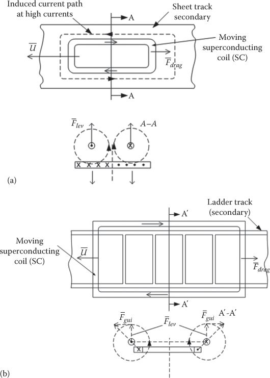
FIGURE 20.1 Normal-flux SC RFLS (only one SC is shown, from a row of NSNS coils): (a) with sheet track and (b) with ladder track.
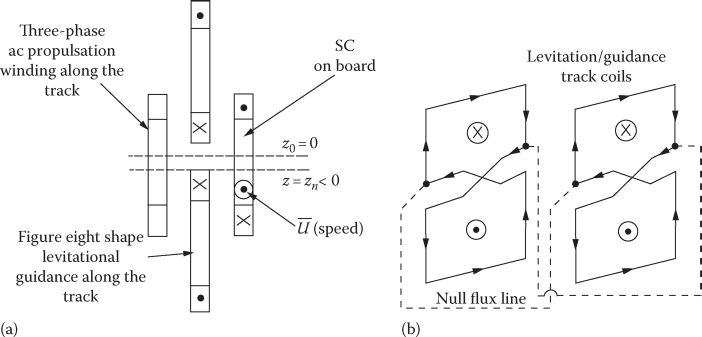
FIGURE 20.2 Null-flux SC-RFLS: (a) transverse cross section and (b) lateral view of light-shape levitation/guidance coils along the track.

FIGURE 20.3 PM-RFLS as magnetic bearing: (a) coil-PM topology and (b) PM + PM + control coil topology.
The competitive technologies in Figures 20.1 through 20.3 may be characterized as follows:
The normal-flux topologies with sheet or ladder track are considered as basic because they reveal the principles and fundamental characteristics: the levitation and eddy currents drag forces, Flev, Fdrag versus speed for various net airgap (levitation height) values in the 50–150 mm range. A levitation goodness factor for forces at peak speed may be defined as
GF=(FlevFdrag)Umax(20.1)
GF=(FlevFdrag)Umax(20.1) The typical system dynamics behavior characterized by static stability but undamped oscillations occurs in the some conditions.
The ladder track is used to increase force goodness factor GF but levitation and drag force pulsations occur, due to ladder transverse currents.
The null-flux systems (Figure 20.2) have been introduced to increase the force goodness factor (which has a notable impact on propulsion power) and to lower the speed at which the peak value of drag force occurs and its value. The neighboring propulsion system ac armature coils may provide repulsive-attractive vertical (and guidance) forces by adequate vector control with controlled id, for damping the levitation vertical or lateral oscillations. Controlled iq is applied for propulsion. A secondary mechanical system is all that is required for meeting the Janeway ride comfort curve (standard).
Note: In Chapter 8, the integrated propulsion/levitation/guidance SC-MAGLEV topology has been presented. The eight-shape stator track coils produce propulsion/levitation/guidance by proper connections and control on the two sides of the vehicle. This topology is not covered here.
Repulsive magnetic PM bearings may be built with an air coil, with controlled current, that repels a moving PM (or vice versa). As the air-coil mmf (and losses) tends to be notable, a dual PM-PM bearing may be built where the control coils (connected together) may be controlled to regulate the system dynamics during rotor motion as well as the takeoff and soft landing at standstill. For this configuration, if the airgap target is not to be tracked with very high precision, the zero (current) power control described in Chapter 19 may be applied as well.
A power levitation goodness factor for levitation and guidance may be defined as
Gp=Flev⋅UFdrag⋅U+Pcontrol(20.2)
Gp=Flev⋅UFdrag⋅U+Pcontrol(20.2) Pcontrol is the control power
Even for a 130 m/s SC MAGLEV, it was demonstrated that force goodness factors in excess of 50/1 may be obtained, while the control power for levitation and guidance may be within 5 kW/ton of vehicle. Zero average current/power levitation control may be attempted provided a dedicated secondary mechanical suspension system damps the vehicle oscillations and a tertiary cabin suspension system provides for ride comfort up to peak speed. The control of vehicle dynamics (except for propulsion) from the propulsion coils on ground reduces notably the power necessary on board of vehicle, which is to be produced by “electromagnetic induction” through dedicated generator coils on board placed between the SCs and guideway.
Superconducting coils may be of low temperature (4–10 K, with liquid helium cooling) and strong or of high temperature and soft (40–70 K, with liquid nitrogen cooling). The appearance of an SC is shown in Figure 20.4a (for basics of superconductivity, see Chapter 1).
In essence, Figure 20.4a comprises the superconducting-wire coil, liquid helium (nitrogen) dewars, fiber glass evacuated insulation, supports, and electrical connections. The helium (nitrogen) dewar is isolated from the environment by a vacuum zone with stainless steel walls around it.

FIGURE 20.4 Superconducting coil: (a) general view and (b) electric power circuit and supply. (After Boldea, I. and Nasar, S.A., Linear Motion Electromagnetic Systems, John Wiley Interscience, New York, 1985.)
For strong SCs, the liquid nitrogen is first poured; after its evaporation, liquid helium is poured until the desired (4-10 K) temperature is reached. Only after that, the electric current is flown into the SC coil gradually; finally, the coil is short-circuited inside the low-temperature structure (Figure 20.4b). The SC may be replenished periodically (after 1 day or more).
20.2 Sheet Secondary (Track) Normal-Flux RFLS
The superconducting coils have large mmf (above (3–4) 105 A turns) as they are supposed to produce in the guideway coils plane NSNS flux densities in the range of at least 0.2–0.3 T for a vertical (lateral) distance of a 0.2–0.3 m (center to center) between the two.
For start, let us consider a coil in air producing a magnetic field in point P (Figure 20.5a). As shown in Chapter 8, by using Biot-Sawart law, via Neumann formula, the magnetic flux density components Bx, By, Bz in point P may be obtained, as illustrated in Figure 20.5b.
The normal (along levitation direction) Bz component for one coil is far from a sinusoid along the vehicle motion direction. However, Bz varies closely to a sinusoid along the lateral direction. A row of SCs may produce, by proper length/width pitching and levitation heights, the desired flux density distribution along all three directions: x, y, z.
The SC field distribution can then be investigated analytically allowing for
Cosinusoidal distribution along oy
Fourier decomposition of longitudinal distribution (along ox) with the retention of fundamental, third, and fifth harmonic
Dependence along oz (vertical) direction results from the Laplace equation and is essentially exponential for each longitudinal harmonic:
∂Hx0∂x2+∂2Hy0∂y2+∂2Hz0∂z2=0(20.3)
∂Hx0∂x2+∂2Hy0∂y2+∂2Hz0∂z2=0(20.3)
with the solutions
Hx0(x,y,z)=∑v=1,3,5Cv0⋅j⋅πvLv⋅e−γv0(z−z0)⋅cos(π2cy)⋅ejπvLvx(20.4)
Hy0(x,y,z)=∑v=1,3,5Cv0⋅j⋅πvLv⋅e−γv0(z−z0)⋅sin(π2cy)⋅ejπvLvx(20.5)
Hy0(x,y,z)=∑v=1,3,5Cv0⋅γv0e−γv0(z−z0)⋅cos(π2cy)⋅ejπvLvx(20.6)
γv0=√(π2c)2+(πvLv)2(20.7)
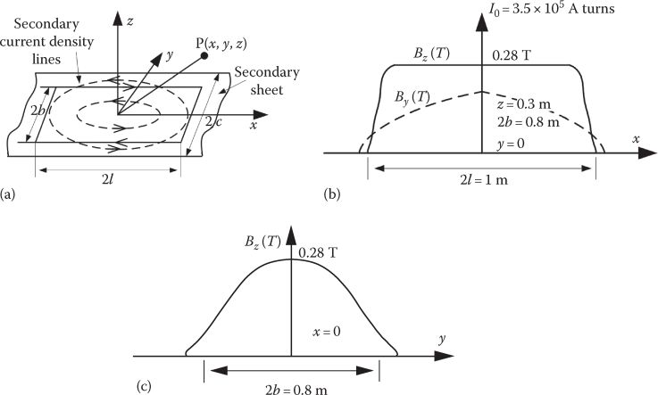
FIGURE 20.5 SC: (a) rectangular coils, (b) Bz and By versus x, and (c) Bz versus y.
To find the integration constants Cv0, we may use another expression of Bz0 = μ0 Hz0 obtained from the Neumann formula (for a rectangular coil) [6]:
Bz0=μ0Hx0=μ0I04π{y+b(y+b)2+z2[x+L/2[(x+L/2)2(y+b)2+z2]1/2−x−L/2[(x+L/2)2(y+b)2+z2]1/2]−y−b(y+b)2+z2[x+L/2[(x+L/2)2(y+b)2+z2]1/2−x−L/2[(x+L/2)2(y+b)2+z2]1/2]}(20.8)
Putting together a few NSNS polarity SCs with a pitch Lv > L (Lv ≈ 1.2 L) and adding their contribution for a given z (height), and at, say, y = 0, after decomposition in Fourier series along X direction, we may identify from (20.6) the integration constants C0v (v = 1, 3, 5). It has been shown that the exponential variation of magnetic field along z (vertical/levitation direction) produces errors within (2%–3%) for z=0.1–0.3 m, SC length L = 1–3 m, and SC width 2b = 0.5–0.8 m.
A similar Poisson field equation is valid for the reaction magnetic field of induced currents in the sheet secondary:
∂2Hrx∂x2+∂2Hry∂y2+∂2Hrz∂z2=−UπvLvσAlμ0Hrz=jUπvLvσAlμ0Hz0(20.9)
If in (20.9) the SC field variation in the sheet secondary is neglected, ∂2 Hrz /∂z2 = 0; (dAL=20–25 mm), the solution of (20.9) simplifies to [6]
Hrz(x,y,z)=∑ν=1,2,5Cνν·Hνz0(x,y,z0)·e−γν(z−z0)·cos(π2cy)·ejπνLνx(20.10)
Hrz(x,y,z)=∑v=1,3,5Cvv⋅Hvz0(x,y,z0)⋅e−γv(z−z0)⋅cos(π2cy)⋅ejπvLvx(20.11)
Hy0(x,y,z)=∑v=1,3,5Cvv⋅Hvy0(x,y,z0)⋅e−γv(z−z0)⋅sin(π2cy)⋅ejπvLvx(20.12)
with
γv|2=γ2v0+jUπvLvμ0σAl;Cvv=−jUvπμ0σAlL⋅γ2v(20.12a)
but Hνz0,Hνy0,Hνx0
The x, y secondary current density lines may simply be calculated as
dA2ˉJ=rptˆHr;dAiˉJx=∂Hry∂y−∂Hrz∂z−;dAi¯Jy=∂Hrz∂z−∂Hrx∂x−(20.13)
For L=2.7 m, Lv = 3 m, I0 = 3 × 10⁵ A turns, 2b = 0.5 m, z0 = 0.25 m, 2c = 0.7 m, dAl=25 mm at U = 10 m/s, and at U = 100 m/s, the variation of induced current density components in the secondary sheet along the direction of motion is as shown in Figure 20.6.
As the secondary sheet thickness is dAl=25 mm, it seems (from Figure 20.6) that the variation of current density along its depth, at high speeds, may not be neglected.
This will be true even for ladder secondary when, to reduce skin effect, a transposed wire conductor has to be used.
Further on, the levitation and drag forces FL and Fd (Figure 20.7) are
FL(u)=μ02⋅N⋅RLv∫0c∫−cz0+dAl∫z0(Jx⋅H*y0−Jy⋅H*x0)dx⋅dy⋅dy =μ0NLvc2∑v=1,3,5C2v0⋅γ2v0⋅Re[Cvvγvγvoγv(1−e−γv⋅dAl)](20.14)
FL(u)=μ02⋅N⋅Re[Lv∫0c∫−cz0+dAl∫z0(Jx⋅H*y0)dx⋅dy⋅dy] =μ0Ncπ2∑v=1,3,5v⋅C2v0⋅γ2v0⋅Re[j⋅Cvvγvγvoγv(1−e−γv⋅dAl)](20.14a)
An attractive method to calculate the levitation force is to start with image levitation force FLi, which is produced by the SC in interaction with its image (Figure 20.8):
FLi=−(∂Wm∂z)I0=ct.=(∂ML∂z)z=2z0(20.15)


FIGURE 20.6 Secondary current density components variation along motion direction, (a) and the variation of Jy along secondary sheet depth, (b) at 10 m/s and at 100 m/s. (After Boldea, I. and Nasar, S.A., Linear Motion Electromagnetic Systems, John Wiley Interscience, New York, 1985.)
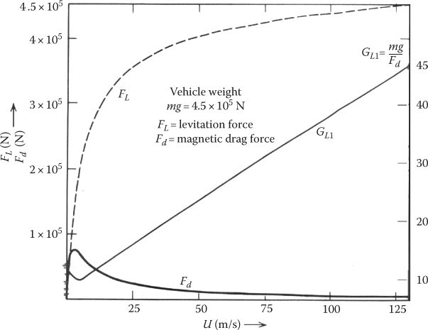
FIGURE 20.7 Levitation FL, drag force Fd, and levitation goodness force factor GL1. (After Nasar, S.A. and Boldea, I., Linear Motion Electric Machines, John Wiley Interscience, New York, 1976.)
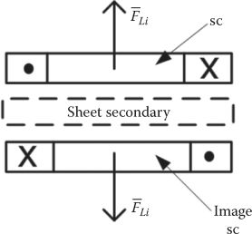
FIGURE 20.8 Image SC.
The variation of levitation and drag force with speed may be approximated as [6]
FL(v)=FLi[1−1[1+(U/U0)2]n1](20.17)
Fd(u)=U0UFL;U≈2μ0σALdAL(20.18)
Analytical 3D or FEM-3D methods may be used to calculate FL(u), Fd(u), and then calibrate Equations 2.17 and 2.18 as practical approximations.
For L = 3 m, 2b = 0.5 m, dAL = 25 mm, z0 = 0.3 m, n1 = 0.2, I0 = 2.315 × 10⁵ A turns, FLi = 55 ton, the results of using (2.17) and (2.18) are shown in Figure 20.7 for a 45 ton vehicle. The results look good, as the peak drag force occurs at a small speed and the levitation goodness factor at 130 m/s is about 45.
The drag power is still about 1.3 MW at 130 m/s, while the air drag of the vehicle is 3 MW.
It is thus evident that sheet guideway solution implies a very high drag power.
Doubling the levitation goodness factor is needed for a competitive MAGLEV. This is how the ladder (coil) secondary was introduced.
20.3 Normal-Flux Ladder Secondary RFLS
The schematics of a ladder secondary are shown in Figure 20.9.
Let us still consider lT, the pole pitch of SCs, and lR, the ladder loop length:
n=lTlR(20.19)
n is the member of ladder loops per SC pole pitch (n > 1).
Also, Lc is the self-inductance of a ladder loop, Moj the mutual inductance of loops o and j. Only the right and left loop interactions are considered here. Rt and Rt are the resistances of longitudinal and transversal sides of the loops.
So the equation of loop o in Figure 20.9 is
Lcddt(io(xo,t))+2Reio(xo,t)+Rt[2io(xo,t)−io(xo−lR,t)−io(xo−lR,t)]−Mcjddtio(xo−lR,t)+io(xo−lR,t)=−ddtΨsc(xo,t)=E(xo,t)(20.20)
where ψsc is the flux of superconducting coils in loop o and E its emf:
E≈∑v=1,3,5Evcos[v(ωt+πxolT)];ω=πulT(20.21)
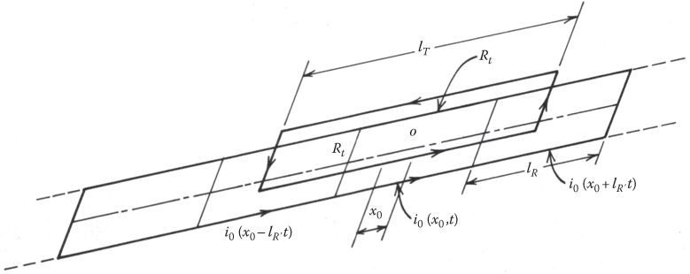
FIGURE 20.9 Ladder secondary schematics. (After Nasar, S.A. and Boldea, I., Linear Motion Electric Machines, John Wiley Interscience, New York, 1976.)
So the induced current in the loop o writes
io(xo,t)≈∑v=1,3,5ivcos(v(ωt+πxolT)−φk)(20.22)
Finally,
io(xo,t)≈∑v=1,3,5Ev(v(ωt+(πxo/lT))−Φk){[2Rl+2Rl(1−cosvπ/n)]2+v2ω2(Lc−2Mc1cosvπ/n)2}1/2(20.23)
with
tan Φk=ωTov(20.24)
and
Tov=v(Lc−2Mc1cos vπ/n)2[Rl+Rl(1−cos vπ/n)]=vLceRce(20.25)
Now the levitation and drag forces for the superconducting coil are
FL(t)=n∑i=1Ioio(m lR,t)∂Mm∂z(20.26)
Fd(t)=n∑i=1Ioio(m lR,t)∂Mm∂x(20.27)
where Mm is the mutual inductance between the SC and m the track loop (m > R for each SC). As expected, the discrete structure of the ladder secondary leads to levitation and drag force pulsations. They should be reduced by proper design; also the peak drag force should be forced to occur at low speeds to facilitate vehicle starting.
For lT = 3.2 m, L = 2.2 m (SC length), 2b = 0.5 m, the harmonics of E are very small. For n = 2 and N-count SCs the forces are obtained from (20.23) to (20.27):
FL≈NMLI2oω2LceR2ce+ω2L2ce∂M∂z(20.28)
Fd≈NMLI2oπLTωRceR2ce+ωL2ce(20.29)
with ML—the mutual inductance between an SC and its image (2.15). For n = 2 and v = 1,
T01=LceRce=Lc2(Rt+Rl)(20.30)
So
FL≈FLiU2U2+(lT/πT01)2;Fd≈FL(ML−∂M/∂z)1T01FLiU2U2+(lT/πT01)2(20.31)
For N = 12 SCs, and the aforementioned data, T01 = 0.15 s, I0 = 2.3 × 10⁵, when the vehicle has 45 ton results as in Figure 20.10 [5] are obtained (−ML/(∂M/∂z) = 0.134 m).

FIGURE 20.10 Ladder secondary normal-flux RFLS: (a) levitation force and (b) drag force Fd and goodness factor. (After Nasar, S.A. and Boldea, I., Linear Motion Electric Machines, John Wiley Interscience, New York, 1976.)
It is clear that the larger the time constant T01, the faster the image levitation force is obtained, however, at increased ladder secondary costs. For a realistic T01 = 0.15 s, the image force is obtained around 200 km/h. The peak value of drag force is only 0.32 × 10⁵ N more than two times lower than for the sheet secondary. Also, the levitation goodness factor reaches a staggering value of 142 at 130 m/s. The force pulsations are small as E1 has small time harmonics, by proper design. The drag power is much smaller than for sheet secondary, but track cost may not be smaller as the manufacturing costs of the ladder secondary tend to be larger.
For even better performance, the null-flux system was introduced.
20.4 Null-Flux RFLS
The null-flux system may be realized with horizontal or with vertical coils; the vertical coil solution is easy to build and handle by the vehicle. The figure-eight-shape secondary is a typical realization of this solution (Figure 20.11).
When the SC is vertically in the horizontal axis of the track coils, the SC flux in the latter is zero. But, as soon as the SC (the vehicle) falls by z0 from that position, the flux is not zero anymore. A net levitation force is produced by the interaction of the SC field with the track-induced currents. Let us denote by M1 and M2 the mutual inductances between the SC and the two parts (upper and lower part) of the eight-shape coils in the track.
Then, proceeding as for the ladder secondary (with n = 2) we may obtain the levitation and drag forces per vehicle as
FLd≈−N(M1−M2)I2oω2LcdR2cd+ω2L2cd∂∂z(M1−M2)(20.32)
Fdd≈N(M1−M2)2I2oωRcdRcd+ω2L2cd;Tcd=Lcd/Rcd(20.33)
Rcd is the resistance of upper (or lower, if equal to each other) track coil and Lcd is the inductance of the same, considering the influence of neighboring track coils.
Taking the same example (lT = 3.2 m, L = 2.2 m, 2b = 0.5 m) with z0 = −2 × 10⁻² m, we may obtain
M1−M2∂M2/∂z−∂M1/∂z≈0.1(20.34)

FIGURE 20.11 Vertical null-flux RFLS.
Following (20.31)
FLd≈−FLiU2U2+(lT/πTcd)2;Fdd≈FLi(M1−M2∂∂z(M1−M2))1TcdU2U2+(lT/πTcd)2(20.35)
This way, the levitation stiffness Sz is
Sz=∂FL/∂zFL(20.36)
and may be calculated as Sz = 12 (it was about 8.0 for the sheet secondary); the peak drag force, for the 45 ton levitation force is now Fdk = 0.228 × 10⁵ N < 0.32 × 10⁵ N of the ladder secondary (so GL > 200!). The levitation goodness factor is thus better. But to obtain the required levitation force, the SC mmf has to be notably larger than for the normal-flux systems.
Note: As shown in Chapter 8, the vertical eight-shape track coils connected to form a nonoverlapping three-phase winding (q = 1/2 slots/pole/phase), and connected across the vehicle to secure guidance higher stiffness, can provide integrated propulsion levitation/guidance.
All done so far in this chapter has paved the way with fields and forces fundamental knowledge to approach this rather complex solution; but it is beyond our scope to follow it farther.
20.5 Dynamics of RFLS
To illustrate the fundamentals of RFLS dynamics, we still use the normal-flux topology, as it is simpler to evaluate the essentials.
Let us consider the SCs of a bogie, on one side, and use the small deviation theory:
z(t)=z0+z(t)(20.37)
The track irregularities are neglected and no other suspension system is considered; the vertical motion equation is
m¨z1=NI20{1−[1+(UUo)2]n1}∂M∂z−mg(20.38)
Notice the ∂M/∂z < 0 with I0 and U as constants:
¨z1=−1mNI20{1−[1+(UUo)2]n1}(∂2ML∂z2)2z0⋅z1(20.39)
In (20.39), it was assumed that FLo = mg.
The solution of (20.39) is evidently sinusoidal:
z1(t)=A cos(γt+Φz)(20.40)
At high speeds, with
γ=[−g(∂2ML/∂z2∂ML/∂z)2z0]1/2;∂2ML∂z2>0
the system stiffness Sz (20.36) is
Sz=∂2ML/∂z2|∂ML/∂z|>0(20.41)
For z0 = 0.3 m and the sheet secondary numerical example in Section 20.2 Sz = 8.0, γ = 8.75 rad, f0 = γ/2π ≈ 1.4 Hz.
The oscillations are not attenuated, and thus the system is dynamically unstable while statically it is stable, as Sz > 0.
This rationale is valid mainly at high speeds. It has been proved that at same speeds [9] there is some positive damping for the ladder secondary (not so for sheet secondary).
20.6 Damping RFLS Oscillations
The oscillations in an RFLS may be damped in three main ways:
Passive electric dampers (PED) (Figure 20.12)
Active electric dampers (AED) (Figure 20.13)
Secondary suspension system (SSS) (Figure 20.14)
Combined passive electric and secondary suspension system (PED + SSS) (Figure 20.15)
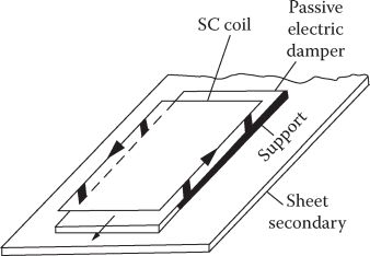
FIGURE 20.12 Passive electric damper sheet. (After Nasar, S.A. and Boldea, I., Linear Motion Electric Machines, John Wiley Interscience, New York, 1976.)
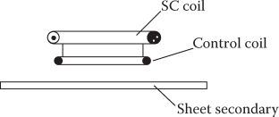
FIGURE 20.13 Active electric damping coil. (After Nasar, S.A. and Boldea, I., Linear Motion Electric Machines, John Wiley Interscience, New York, 1976.)
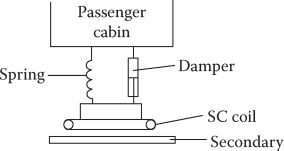
FIGURE 20.14 Secondary suspension system (SSS).
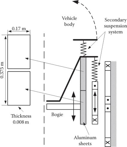
FIGURE 20.15 Combined SSS and passive electric damper sheet placed on the bogie.
A short characterization of the solutions reveals the following:
It has been shown that PED, consisting of a conducting plate (or shorted coil) placed between the SC and the guideway, is able to produce a damping time constant τ < 1 s only if the distance between the SC and PED is at least 0.15 m [10]. This leaves 0.02–0.05 m vehicle-guideway airgap and thus imposes lower irregularity (higher costs) track, to avoid collisions. Also, below 2 Hz PED is not able to damp the SC oscillations.
The active electric damper is supposed to be capable of damping the MAGLEV oscillations and assure enough ride comfort, but at notable energy consumption on board; this solution will be detailed later.
The active (controlled) pneumatic SSS is also capable of damping oscillations and providing full ride comfort up to the maximum vehicle speed [11]; being fully mechanical, it is not followed here in more detail.
The PED + SSS (passive) system may be capable of damping the vertical oscillations and providing ride comfort from 1 Hz onward [12,13] at reasonable initial system costs. This solution will also be treated here in the same detail. For a thorough synthesis on dynamics and stability of RFLS, see Ref. [13].
20.6.1 Active Electric Damper
Let us start with levitation force approximate linearized expression for a normal-flux RFLS [6]:
FL≈FLi⋅ω2τ21+ω2τ2[1−2γ10z1(t)−1ω2τ⋅(1−ω2τ2)(1+ω2τ2)˙z1(t)](20.42)
τ = Le/Re equivalent electric time constant for sheet or ladder guideway coils, FLi —image levitation force and ω = π•U/Lv is related to vehicle speed; z1—vertical airgap deviation from linearization value z0; γ10 = π/Lv.
If we add now a control coil fixed below the SC, at zc height, the motion equation of the SC is
m¨z1=FL−mg−2Ic(t)Io(∂M′Lc∂z)z0+zc⋅ω2τ21+ω2τ2(20.43)
Ic(t) is the control coil current and M′Lc
To damp the vertical oscillations, the control current is proposed to be
Ic(t)=αc˙z1(t)−kz1(t)(20.44)
This control law of current presupposes that the value of z1(t) may be measured and ⌢˙z1(t)
Introducing (20.44) in (20.43), one obtains
m¨z1(t)+ω2τ21+ω2τ2[2FLiγ10−2KzIo(∂M′Lc∂z)z0+zc]⋅z1(t) +[γ10ω2τFLi(1−ω2τ2)(1+ω2τ2)+2αvIo(∂M′Lc∂z)z0+zc]˙z1(t)=0(20.45)
The solution of (20.46) should be a damped oscillation—for stable operation—with a time constant τd and a frequency ω0:
z1(t)=z0e−t/τd cosω0t(20.46)
with
τd=2⋅mω2τ21+ω2τ2[γ10ω2τFLi(1−ω2τ2)(1+ω2τ2)+2αvI0(∂M′Lc∂z)z0+zc](20.47)
and
ω0={ω2τ2[2γ10FLi−2KzI0(∂M′Lc/∂z)z0+zc]m(1+m2τ2)}1/2(20.48)
With ω20<0
Finally, from (20.46) to (20.47) we calculate αv = 1.33 × 10⁴ (As/m); Kz = 1.16 × 10⁵ (A/m).
The position z1(t) and acceleration response z1(t) for a sudden (step) change in position of zi = 0.03 m are shown in Figure 20.16:
z1(t)=zi(cosω0t+sinω0tτdω0)e−t/τd(20.49)
It must be seen that the response is periodic and attenuated. The frequency response not only to vertical position modifications but to external perturbations such as wind gusts or track irregularities at various speeds is required before deciding that AED is suitable for a practical system.
Here we investigate only the response to guideway irregularities as it is related to ride comfort.

FIGURE 20.16 Active electric damper response to step change reference position of zi = 0.03 m at 100 m/s: (a) vertical position response and (b) vertical acceleration response. (After Nasar, S.A. and Boldea, I., Linear Motion Electric Machines, John Wiley Interscience, New York, 1976.)
20.6.2 AED Response to Guideway Irregularities
The guideway irregularities may be considered sinusoidal (as done for attractive force levitation systems):
z0=zgsinωt(20.50)
where zg is
zg=[∞∫ΩiΨ(Ω′)dΩ′]1/2; Ψ(Ω)=AΩ′2; Ω′=2πf/U(20.51)
with f as the frequency of oscillations.
Detailing from zg in (20.51) yields
zg=[f∫0.2AU2πf2df]1/2(20.52)
If this perturbation is introduced in Equation 20.45, its solution becomes
z1(t)=zasin(ωt+φi)+A1e−t/τdcos(ω0t+φ0)(20.53)
za=zg(ω20+1/τ2d)sinφi|ω2|tanφi+2ω/τd−ω20−1/τ2d(20.54)
φi=tan−12ω/τdω2−(ω20+1/τ2d)(20.55)
With zero initial conditions A1 and φ0 may be calculated:
tanφ0=ω cos φi+(1/τd)sinφiω0sinφi(20.56)
A1=−zasin φisin φ0(20.57)
Knowing z1(t) we can calculate ˙z1(t)

FIGURE 20.17 AED response to track irregularities at 100 m/s: (a) acceleration response and (b) control coil mmf requirement. (After Nasar, S.A. and Boldea, I., Linear Motion Electric Machines, John Wiley Interscience, New York, 1976.)
This amounts to about a maximum of 5 kW/ton, which is about in the range of attractive force levitation systems at 100 m/s.
This simplified analysis of AED may serve as a preliminary design basis, as for an actual system a multitude of other factors have to be included [13].
20.6.3 PED + SSS Dampers
As alluded to in Figure 20.15, a combination of an aluminum double sheet (one upper, one lower, 0.008 m thick), placed on the MAGLEV bogie, and the SCs fixed to the bogie and to passenger cabin by a mechanical suspension system, may be able to produce stable operation for the vertical motion (levitation) in an eight-shape (null-flux) RFLS with vertical SCs [12].
FEM computation results for an assumed vertical motion of SC at 10 Hz for an amplitude of 0.02 m have led to a vertical (levitation) force as in Figure 20.18a [12] for a full-size MAGLEV.

FIGURE 20.18 AED+SSS system (a), stiffness K (b), damping coefficient versus frequency (c). (After Miikura, S. et al., Electromagnetic stiffness and damping effects in the secondary suspension of a superconducting MAGLEV vehicle, Record of LDIA-1995, Nagasaki, Japan, pp. 97–100, 1995.)
The force seems rather sinusoidal and thus a single eddy current mode (harmonic) suffices. Therefore, for the bogie-attached aluminum sheet, the circuit equation is
Ldidt+Ri=E; E=∂M∂z⋅I0⋅˙Zsc(20.58)
In (20.58), the SC mmf was considered constant.
The vertical force Fz between the SC and bogie-attached aluminum sheet is
Fz=−∂M∂ziI0(20.59)
As Fz from FEM varies sinusoidally in time, it may be represented in complex numbers:
Fz=(∂M∂z)2I20Rjωjωτ+1≈(k+jωc)zc(20.60)
The time constant τ results from fitting (20.60), with the FEM force Fz in Figure 20.18a as
|Fz|=αωzmax√ω2τ2+1; zmax−SC motion ampliude(20.61)
The system stiffness and damping coefficients are shown in Figure 20.18b,c.
For 20 Hz, the stiffness K increases with frequency and it is 2.7 × 10⁵ N/m, which is about 30% of the mechanical stiffness of the air spring system attached to the SCs. Whether this performance is good enough to provide for the ride comfort, up to maximum speed, with the contribution of SSS, remains to be proven; but the rather constant frequency damping coefficient from 1 Hz is a beneficial property of it.
Note: Active electric damping of vertical motion can be done through the vector control of propulsion by nonzero id control in an integrated levitation (propulsion) guidance with vertical coils on the sides of a U-shape guideway.
While previously we treated the fundamentals for 1 DOF systems, the dynamic of a passive 5 DOF–RFLS is treated in Refs. [14–17]. More on these aspects will be found in a chapter on active guideway MAGLEVs.
20.7 Repulsive Magnetic Wheel
The superconducting paddle wheel vehicle, Cryobus (Figure 20.17) [6], was earlier proposed for MAGLEVs [18].
The configuration of Cryobus as in Figure 20.19 may be characterized as follows:
The superconducting heteropolar SC wheels are rotated over a triple ladder or triple short-circuited coil raw, placed along the track, to produce propulsion (much like a linear air-coil induction motor), levitation, and guidance by repulsive forces; a mechanical active secondary system is to be designed to damp oscillations for a safe and comfortable ride.
The magnetic wheels produce propulsion/levitation/guidance as long as ac is produced in the guideway; it means that by spinning the wheel at, say, nonzero slip frequency the MAGLEV might develop enough force to lift the vehicle at zero speed. To provide lift force at zero propulsion force, we simply rotate half of the wheels in one direction and the rest in the opposite direction. So, theoretically the takeoff may take place from standstill.
When the wheel peripheral speed Uwp is larger than the vehicle speed U, the propulsion force is positive while for Uwp < U regenerative braking is produced.
As only the lower half of the wheel interacts with the guideway, the upper half may interact with arch-shape synchronous motor ac stator windings, to “paddle” the magnetic wheel, and save space and hardware. With 2p = 8 poles, 4 poles may be used to “paddle” the wheel.
The free rotating copper cylinder, Figure 20.17b, may be used to damp the oscillations in levitation (as PED).
As the magnetic coupling between the circular wheel and the flat guideway is weaker than for flat SCs, the overall efficiency of Cryobus is expected to be lower than for flat-coil RFLS–MAGLEVs. However, when used to integrate proportional levitation guidance functions, the Cryobus may attain a total power efficiency up to 65% and thus compete with electrodynamic flat-coil active guideway MAGLEVs in a simpler topology (see Ref. [6], Chapter 12, for preliminary design).
The Cryobus needs all power to be transferred on board of vehicle as the track is passive, and thus it may prove to be an overall cost/performance solution worth reconsideration.
Recently, the superconducting wheel has been proposed to be replaced by a heteropolar PM wheel [19,20]. The same concept was proposed to compensate the dynamic end effect in high-speed LIMs. If the PM wheel could duplicate the performance of the SC dual-axial-pole wheel (Figure 20.17b) with a higher than 1.5 T remanent flux density, then this latter solution might stand a practical application challenge, even if flying at a smaller height (0.04–0.06 m).
In general, the replacement of SCs by strong PMs is so far less practical because of the lower weight of SCs at 0.15–0.2 m rated gap for given lift force. But stronger PMs of the future at smaller gap might reverse the situation soon [21,22].
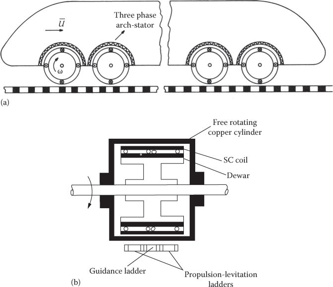
FIGURE 20.19 Cryobus longitudinal view, (a) and cross-section of the paddle wheel, (b). (After Nasar, S.A. and Boldea, I., Linear Motion Electric Machines, John Wiley Interscience, New York, 1976.)
20.8 Coil-PM Repulsive Force Levitation System
The experimental setup in Figure 20.20 [23] may be applied directly to an industrial MAGLEV platform or to an axial bearing of an air-core PM synchronous motor/generator inertial battery. In contrast to attraction force levitation systems, it allows long (up to 20 mm or more) excursion length.
To analyze the dynamics of this 1 DOF system with vertical position tracking control, the motion equation including coil force, gravity, friction, and external force disturbance is used:
FL−m⋅g−B⋅˙x−Fext=m⋅¨x(20.62)
where
x is the vertical distance between PM and air coil
m is the PM mass
B is the friction coefficient
FL is the levitation (repulsive) force of coil current
Fext is the external force disturbance
If V(t) is the control effort, the levitation force may be approximated as follows [23]:
FL≅V(t)a(x+b)4(20.63)
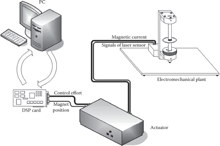
FIGURE 20.20 Coil-PM repulsive force levitation system. (After Slotine, J.J.E. and Li, W., Applied Nonlinear Control, Prentice-Hall, Englewood Cliffs, NJ, 1991.)
With and, after separating the time varying uncertainties, from lumped uncertainties L(x,t), Equations 20.62 and 20.63 may be put in the form
¨x(t)=fn(x¯,t)+Gn(x¯,t)⋅V(t)+dn(x¯,t)+L(x,t)(20.64)
with
L(x¯,t)=Δf+ΔGV(t)+Δd<δ(20.64a)
For robust control, the sliding mode control approach is corroborated here with a radial basis function network (RBFN), to estimate online the uncertainties in the system dynamics.
The sliding mode functional S(t) is standard:
S(t)=˙e(t)+λ1e(t)+λ2t∫0e(τ)dτ; e(t)=x*−x(20.65)
The values of λ1 and λ2 represent the desired dynamics and may be calculated from given rise time and overshooting as in a second-order system. The globally asymptotic stability may be guaranteed (based on the Lyapunov method) with a control law of the form
V(t)=G1n(x,t)[−fn(x¯,t)−dn(x¯,t)+¨xm−λ1˙e(t)−λ2e(t)−δ⋅sign⋅S(t)](20.66)
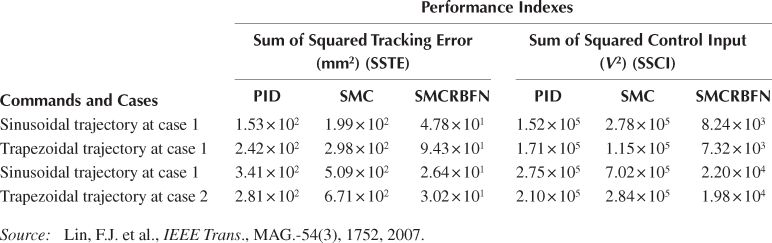
Following the approach with the RBFN estimator, for m = 0.121 kg, B = 2.69, a = 1.65, b = 6.2, λ1 = 10, δ = 10, λ2 = 30, results as in Figure 20.21 and Table 20.1 [24] have been obtained.
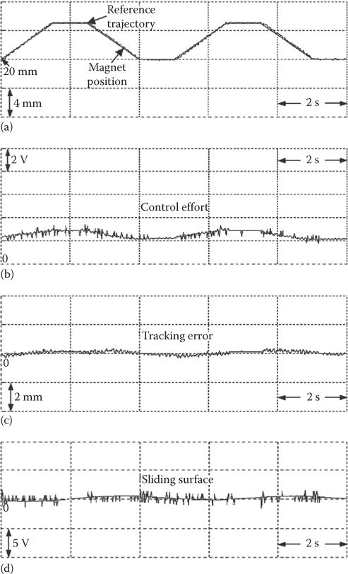
FIGURE 20.21 Experimental results for trapezoidal airgap command: (a) reference and actual position, (b) control effort, (c) tracking error, and (d) sliding surface. (After F.J. Lin et al., IEEE Trans., MAG-54(3), 2007, 1752.)
TABLE 20.1
Control Performance
The response is stable, the position tracking quality is good, and the control effort is reasonable for a large airgap.
The synthetic results in Table 20.1 [24] compare PID, SMC, and SMC-RBFN control systems and demonstrate that the SMC-RBFN performs best on an overall basis. An alternative adaptive back-stepping intelligent control system for the same prototype [7] has been shown to track complex position/time waveforms rigorously.
Still, the results in position tracking refer to small frequency bands, and further investigations into high-frequency band position control are needed for dynamically critical applications.
20.9 PM-PM Repulsive Force Levitation System
In the search for high rigidity (stiffness), the PM-PM RFLS has been proposed for axial bearings. To operate with no (or minimum) control, the repulsive force is beneficial as it provides static stability; it does not provide positive damping in general. However, as discussed previously in this chapter, the passive small resistance electric damper may help to produce positive damping in such applications where the axial speed is small. So, either PED or AED may be used in a PM-PM RFLS (Figure 20.22).
The multiple PM disks (12, 24, etc.) are mounted in the aluminum plates (Figure 20.22). The number of PM disks per circle, their thickness, and the diameters of their placing on stator and rotor may be used for optimal design and stability. For a simplified analytical model, the magnets in air may be replaced by their intensities F1 = Hc A2 and F2 = HcA2, where Hc is the coercive magnetic field (say Hc = 1.78 × 10⁶ A/m), residual flux density Br = 1.08 T (approximately μrec = 1 p.u.); A1 and A2 are the PM pole force areas. The PM pole intensity is considered as concentrated in the center of the PM pole. The force is
ˉF=μ0F1F204π⋅r212ˉu12(20.67)
where r12 is the distance between the PM pole centers.
The number of PM disks on rotor and stator per circle is the same; ˉu12
For a certain z/hPM and PM radial length/z, the repulsive force will be maximum.
Concerning the radial force, it has to be negative (centralizing) for stable guidance, and this happens only for small radial displacements in combination with lower rotor than stator diameter of placing the PMs.

FIGURE 20.22 PM-PM repulsive force levitation system: (a) with passive (aluminum plate) damper and (b) with active electric damper.

FIGURE 20.23 PMs as air coils.
For hPM = 10 mm, at z = 2.5 mm, the repulsive force, for Dr = 47.5 mm and Ds = 50 mm, is maximum at 23 N [8], while the radial force is negative up to 1 mm radial displacement, but only at –0.5 N. When the rotor rotates, the 24 PMs on both rotor and stator assume different relative positions and thus the repulsive (vertical) levitation force pulsates heavily even with Dr = 74.5 mm and Ds = 50 mm (± 6 N).
However, much like for cogging force, if the number of PMs on stator and rotor is different (say 26/24), the levitation force pulsations during rotor rotations become small; alternatively, with two out of phase rows of PMs on the stator at Ds1 = 50 mm and Ds2 = 45 mm, with Dr = 47.5 mm, and 24 PMs on both rotor or stator, the repulsion force pulsations become small. While in principle the PM-PM RFLS works, there is still a lot of work to be done to
Analyze it by 3D-FEM
Elaborate an optimal design code to check the performance/cost
Include the eddy currents in the aluminum plates
Develop a state space circuit model for dynamics and control
Investigate static and dynamic stability
Introduce oscillation passive damping or closed-loop control via coils for refined levitation height tracking [25]
All the aforementioned issues are beyond our scope here, but seem worthy of further consideration by the interested reader.
20.10 Summary
Repulsive (electrodynamic) force may be developed in practical devices between
Conductors carrying currents of opposite polarity
A moving current carrying (or superconducting or a PM) coil raw and a fix secondary conducting sheet or ladder
Two rows of PMs of opposite polarity
One row of PMs and controlled current air coils
The repulsive force tends to separate the two bodies with an intensity that increases when the distance (air gap) between the two decreases. It is thus statically stable. This is in contrast to attraction force levitation systems (AFLSs), which are statically unstable.
Large repulsive forces may be produced with strong PMs or superconducting coils at air gaps 10 times larger than for AFLS (where 10–15 mm is typical); this way the track irregularities may be larger and thus lower costs are expected.
As levitation means statically and dynamically stable hovering of a body (e.g., a MAGLEV), the dynamics and some control for repulsive force levitation system have to be investigated.
For MAGLEVs, RFLS have been proven practical up to 585 km/h.
The RFLS is in general based on the interaction of superconducting coils (SCs) on board of vehicle to produce 0.3–0.6 T flux density in the plane of secondary (track) conducting sheet, ladder, or eight-shape short-circuited coils placed along the guideway of MAGLEV.
Normal-flux RFLS have been proposed first, but the null-flux eight-shape short-circuited vertical coil guideway has been proven the overall best solution for integrated levitation guidance and propulsion.
To investigate the fundamentals of RFLS with SCs, the normal-flux topologies with sheet or ladder secondary have been investigated in some detail.
As expected, when a row of SCs with NSNS polarity on board of MAGLEV moves above a sheet or ladder guideway, induced currents occur in the latter.
As the speed increases, the frequency of these currents increases and thus their circuit becomes more and more inductive; at high speeds, the induced currents look almost opposite in polarity to those in the neighboring SC. This indicates a strong repulsive (levitation force) FL. But a drag force Fd corresponds to the losses in the conducting guideway.
While the levitation force grows monotonously with speed U, the drag force shows a peak value with speed, much like the torque in a dc stator–fed induction motor with cage rotor.
Two criteria have been introduced to weigh the levitation “goodness”: levitation force goodness (FL/Fd)umax and levitation power goodness FL⋅U(Fd⋅U+Pcontrol)
FL⋅U(Fd⋅U+Pcontrol) , where Pcontrolis the dynamic (control) power needed to replenish the SCs and for motion dynamic stabilization and control. The higher the two criteria values the better for some given initial system costs.Using a larger airgap than AFLS, the RFLS with SCs has been so far proven, at higher SCs length, capable to produce better performance at higher speeds (up to 585 km/h); the SCs volume for same levitation force tends to be smaller than that of dc-controlled iron-core coils.
But the levitation force increases with speed, and the critical speed at which the drag force has its peak values leads to the conclusion that the vehicle has to start and accelerate on retractable wheels (much like an aircraft, while AFLSs work as helicopters do).
For 3 m long, 0.5 m wide SC coils, RFLS have been built to produce (FL/Fd)130 m/s above 50/1 for sheet guideway, 120/1 for ladder guideways, and above 200/1 for null-flux (eight-shape track coils) systems.
An analytical study of RFLS showed that by careful design SC flux in the track (sheet or ladder type) may vary almost sinusoidally in time. Also, the SC flux density in the guide-way plane varies rather cosinusoidally along the transverse direction. Consequently, the vertical force flux density varies along the airgap exponentially. A practical field theory may be obtained to produce levitation and drag force dependence on speed and on system geometry. Curve fitting may be used to match these theoretical results to the image levitation force based (Neumann) formula and a proposed speed dependence.
A similar (but based on circuit theory) model for the ladder and null-flux guideway system is obtained. In this case, however, additional pulsations in Fc and Fd occur; by a proper design, they may be reduced to negligible values.
This way the aforementioned high levitation force goodness values have been obtained.
Using these models in the motion equation (of a 1 DOF system), it is proven that the self-damping coefficient is negative at all speeds for the sheet guideway and above a small speed (15–25 m/s) for the ladder or null-flux guideway.
Damping these natural (inherent) oscillations may be accomplished by
Passive electric damper (PED)
Active electric damper
Mechanical damper
Combined passive (on bogie) electric and mechanical damper
PEDs are in general incapable of damping vehicle oscillations properly for the entire frequency spectrum or providing ride comfort up to maximum speed.
The active electric damper with a room temperature controlled coil on board, placed between the SCs and the guideway, has been shown to be capable of producing satisfactory ride comfort up to maximum speed for a maximum of 5% of SC mmf in the control coil. An average of 5 kW/ton of control power is required at 550 km/h. This is only 40% more than the control power in AFLS at 360 km/h.
The ride comfort is still defined by the Janeway curve, which limits acceleration versus frequency due to track irregularities (up to 20 Hz).
Even the passive electric damper (two vertical aluminum sheets on the bogie, parallel to SC) with a secondary suspension system of SCs to bogie and cabin seems capable of providing good oscillation damping from 1 Hz upward.
In the null-flux RFLS, when the eight-shape track coils are connected as a three-phase ac winding (with q = 1/2 slots/pole/phase), and with connections of the coils on the two sides of the vehicle, integrated levitation and propulsion are obtained. This time vector control of the of the ac three-phase windings (as in a linear synchronous motor—Chapter 8) will control propulsion by iq control and stabilize the vertical vehicle oscillations by id control, instead of AED. Zero levitation power control may be attempted for RFLS as for AFLSs.
The heteropolar SC or PM wheel on board rotating at Uw > U peripheral speed above a track sheet or ladder can be designed to produce integrated levitation/propulsion/guidance at a smaller airgap (0.04–0.06 m). The upper half of so-called magnetic wheel is driven by a three-phase arch-shape stator much like in a rotary synchronous motor. A passive guide-way MAGLEV is thus produced. Due to the smaller region of interaction, that is, weaker interaction of magnetic wheels with the guideway, the PMs (SCs) mmf has to be stronger than for flat RFLS of the same performance. Horizontal magnetic wheels with PMs and vertical axis with partial overlapping of guideway conductive sheets or ladders have also been proposed for RFLS [26].
For standstill (bearings) or industrial MAGLEV platforms, repulsive force levitation may be produced by moving PMs and fix controlled current coils (much like for planar motion linear electric motors). Sliding mode control has proven very effective to track airgaps around 20 mm with good precision in such systems.
PM-PM repulsive force levitation has also been proven adequate, with limited range lateral stabilization and passive (aluminum plate) damping, in axial bearings with rotors rotating at large speeds; active (close-loop) control is required to fully control such systems.
It is estimated here that R&D on RFLS will develop quickly in the near future, both for super high-speed transport and for industrial applications (bearings and industrial MAGLEV platforms in clean rooms).
References
1. G.T. Danby and J.P. Powell, Integrated systems for magnetic suspension and propulsion vehicles, Record of Applied Superconductivity Conference, Annapolis, MD, 1970.
2. J.R. Reitz, R.H. Borcherts et al., Preliminary design studies of magnetic suspensions for high speed transportation, Final Report DOT-FRA-10026, Washington, DC, March 1973.
3. T. Yamada and M. Iwamoto, Theoretical analysis of lift and drag forces on magnetically suspended high speed trains, Electr. Eng. Jpn., 92(1), 1973, 53–61.
4. E. Ohno, M. Iwamoto, and T. Yamada, Characteristics of Superconducting magnetic suspensions and propulsion for high speed trains, Proc. IEEE, 61(5), 1973, 579–586.
5. S.A. Nasar and I. Boldea, Linear Motion Electric Machines, Chapter 7, John Wiley Interscience, New York, 1976.
6. I. Boldea and S.A. Nasar, Linear Motion Electromagnetic Systems, Chapter 11, John Wiley Interscience, New York, 1985.
7. F.J. Lin, L.T. Teng, and P.H. Shieh, Intelligent adaptive backstepping control for magnetic levitation apparatus, IEEE Trans., MAG-54(5), 1973, 579–586.
8. S.C. Mukhopadhyay, J. Donaldson, G. Sengupta, S. Yamada, C. Chakraborthy, and D. Kacprzak, Fabrication of a repulsive-type magnetic bearing using novel arrangement of PM for vertical rotor suspension, IEEE Trans., MAG-39(5), 2003, 3220–3222.
9. T. Yamada, M. Iwamoto, and T. Ito, Magnetic damping force in inductive magnetic levitation system for high speed trains, Electr. Eng. Jpn, 94(1), 1974, 80–84.
10. M. Iwamoto, T. Yamada, and E. Ohno, Magnetic damping force in electrodynamically suspended trains, IEEE Trans., MAG-10(3), 1974, 458–461.
11. R.H. Borcherts et al., Preliminary design studies of magnetic suspension for high speed ground transportation, Record of FRA, PB. 224 843, Washington, DC, June 1974.
12. S. Miikura, A. Kameari, M. Igarashi, and J.I. Kitano, Electromagnetic stiffness and damping effects in the secondary suspension of a superconducting MAGLEV vehicle, Record of LDIA-1995, Nagasaki, Japan, pp. 97–100, 1995.
13. D.M. Rote and Y. Cai, Review of dynamic stability of repulsive-force MAGLEV suspension systems, IEEE Trans., MAG-38(2), 2002, 1383–1390.
14. A. Seki, Y. Osada, J.I. Kitano, and S. Miyamoto, Dynamics of the bogie a MAGLEV system with guide-way irregularities, IEEE Trans., MAG-32(5), 1996, 5043–5045.
15. J. de Boeij, M. Steinbach, and H.M. Gutierrez, Mathematical model of the 5 DOF sled dynamics of an electrodynamic MAGLEV system with a passive sled, IEEE Trans., MAG-41(1), 2005, 460–465.
16. J. de Boeij, M. Steinbach, H.M. Gutierrez, Modeling the electromechanical interactions in a null-flux electrodynamic MAGLEV system, IEEE Trans., MAG-41(1), 2005, 466–470.
17. R.D. Kent, Designing with null flux coils, IEEE Trans., MAG-33(5), 1997, 4327–4334.
18. L.C. Davis and R.H. Borchers, Superconducting paddle wheels, screws and other propulsion units for high speed ground transportation, Scientific Research Staff, Ford Motor Co., Dearborn, MI, January 22, 1973.
19. N. Fujii, Y. Ito, and T. Yashihara, Characteristics of a moving magnet rotator over a conducting plate, IEEE Trans., MAG-41(10), 2005, 3811–3813.
20. J. Bird and T.A. Lipo, An electrodynamic wheel: An integrated propulsion and levitation machine, Record of IEEE IEMDC-2003, pp. 1410–1416.
21. W. Ko and C. Ham, Novel approach to analyze the transient dynamics of an electrodynamics suspension MAGLEV, IEEE Trans., MAG-43(6), 2007, 2603–2605.
22. Q. Han, C. Han, and R. Philips, Four and eight-piece Halbach array analysis and geometry optimization for MAGLEV, IEE Proc., EPA-152(3), 2005, 535–542.
23. J.J.E. Slotine and W. Li, Applied Nonlinear Control, Prentice-Hall, Englewood Cliffs, NJ, 1991.
24. F.J. Lin, L.T. Teng, and P.H. Shieh, Intelligent sliding-mode control using RBFN for magnetic levitation system, IEEE Trans., MAG-54(3), 2007, 1752–1762.
25. S.C. Mukhopadhyay, T. Ohji, M. Iwahara, and S. Yamada, Design analysis and control of a new repulsive type magnetic bearing, IEE Proc., EPA-146(1), 1999, 33–40.
26. N. Fujii and S. Nonaka, Payload of revolving PM type magnet wheel, Record of LDIA-1998, Tokyo, Japan, pp. 351–354, 1998.