Chapter 10 Linear Reluctance Synchronous Motors: Modeling, Performance Design, and Control

Search in book...
Toggle Font Controls
Create new playlist

Name your new playlist

Playlist description (optional)
Sign In

Email address

Password

Forgot Password?

or

Continue with Facebook

Continue with Google
Sign Up

Full Name

Email address

Confirm Email Address

Password

or

Continue with Facebook

Continue with Google

Modeling, Performance Design, and Control

Linear reluctance synchronous motors (L-RSM) are characterized by a short primary magnetic core with uniform slots that host a distributed three-phase ac winding and a long variable reluctance (magnetically anisotropic) secondary (Figure 10.1a and b). The distributed three-phase ac windings produce a traveling magnetic field in the airgap; its inductances (self and mutual) vary rather sinusoi-dally with 2θ_er (θ_er rotor electrical angle between phase a axis and the secondary d (high inductance) axis). The key to high performance is a high ratio (and difference) between d and q axis synchronous inductances: an L_d/L_q ≥ 3 is a minimum requirement, but L_d/L_q > 7 (8) would be desirable.

Essentially, there are two main applications, which refer to

Medium- and high-speed transportation
Low-speed short travel industrial applications

The configuration in Figure 10.1a, especially with segmented-laminated secondary, may be considered for medium- and high-speed MAGLEVs (g = 6 ÷ 10 mm) even if only moderate saliency is obtained (L_d/L_q=2.5 ÷ 3.5), because its large normal force serves to levitate the vehicle, “saving” thus the rather low power factor at an acceptably good efficiency, for a reasonably low-cost passive guideway, but for a more expensive PWM inverter on board (higher kVA). In contrast, the multiple flux barrier (MFB) secondary or axially laminated secondary (Figure 10.1b) produces larger saliency for a low airgap, g = 0.5 ÷ 1 mm for short travel (a few meters), heavy weight load transporters (primaries), fed from a mechanically flexible ac power cable.

Note: The MFB (higher saliency) secondary may also be used for large airgaps (g = 6 ÷ 10 mm), but for long travel (tens or hundreds of kms), the track cost is increased significantly, though a better power factor means a lower cost and weight of the on-board PWM inverter.

The long primary/short secondary mover topology has to be ruled out for L-RSM due to the “vanishing” of the magnetic saliency (L_d/L_q = 1.1 1.15) and thus operation at very low power factors (0.1 0.2) and, consequently, at huge kVA rating of on-ground PWM inverter sections.

10.1 L_dm, L_qm Magnetization Inductances of Continuous Secondary (Standard) L-RSM

Intuitively the derivation of L_d and L_q should start with the fundamental airgap flux density produced by the primary mmf in the airgap in axes d and q, B_ad₁, B_aq₁, and then compare them with the same but produced for a uniform airgap g₁, B_a₁. The magnetization inductances would then be

L d m = B a d 1 B a 1 \cdot L m = k d m 1 \cdot L m; L q m = B a q 1 B a 1 \cdot L m = k q m 1 \cdot L m (10.1)

$L_{d m} = \frac{B_{a d 1}}{B_{a 1}} \cdot L_{m} = k_{d m 1} \cdot L_{m}; L_{q m} = \frac{B_{a q 1}}{B_{a 1}} \cdot L_{m} = k_{q m 1} \cdot L_{m} (10.1)$

Images

FIGURE 10.1 Practical L-RSM topologies: (a) with low saliency (for large airgap: g > 1 mm) and (b) with higher saliency (for smaller airgap: g < 1 mm).

L m = 6 μ 0 ( W 1 k W1 ) 2 τ \cdot L π 2 p . k C \cdot g 1 ( 1 + k s ) (10.2)

$L_{m} = \frac{6 μ_{0} {(W_{1} k_{W1})}^{2} τ \cdot L}{π^{2} p . k_{C} \cdot g_{1} (1 + k_{s})} (10.2)$

where

W₁ is the turns/phase in series

kW1 $k_{W_{1}}$ is the fundamental winding factor (kW1=kq1⋅ky1⋅kskew $k_{W_{1}} = k_{q 1} \cdot k_{y 1} \cdot k_{s k e w}$ )

τ is the pole pitch of ac winding and of secondary saliency

L is the stack length

g₁ is the mechanical gap

k_S is the magnetic saturation factor k_S = 0.1 ÷ 0.2 for large airgap machine

The coefficients k_dm₁, k_dm₁ for the conventional salient-pole continuous (laminated) secondary (Figure 10.1a) are approximately [4]

K d m 1 \approx g 1 g 2 + (1 - g 1 g 2) (τ p τ + 1 π sin π τ τ p) (10.3)

$K_{d m 1} \approx \frac{g_{1}}{g_{2}} + (1 - \frac{g_{1}}{g_{2}}) (\frac{τ_{p}}{τ} + \frac{1}{π} \sin \frac{π}{τ} τ_{p}) (10.3)$

K q m 1 \approx g 1 g 2 + (1 - g 1 g 2) (τ p τ - 1 π sin π τ τ p) (10.4)

$K_{q m 1} \approx \frac{g_{1}}{g_{2}} + (1 - \frac{g_{1}}{g_{2}}) (\frac{τ_{p}}{τ} - \frac{1}{π} \sin \frac{π}{τ} τ_{p}) (10.4)$

For large airgap (g₁ = 10 mm), τ_p/τ = 0.66; g₂ = 5g₁ (to reduce secondary weight), k_dm₁ = 0.9467 k_qm₁ = 0.484. Only a saliency ratio L_dm/L_qm = 1.956 is obtained. This will eventually lead to a power factor below 0.4, and the secondary height h_sec=τ/2π+6 • g₁ is large and thus costly (and heavy).

Note: For a small airgap (g = 0.4 ÷ 0.5 mm) and a pole pitch τ ≥ 0.06 m, the low power factor may be acceptable (as for LIMs) in short travel, small-speed (even at 5 Hz) direct drives due to the simplicity of the secondary and its small cost.

10.2 L_dm, L_qm Magnetization Inductances for Segmented Secondary L-RSM

In an effort to increase magnetic saliency ratio (L_dm/L_qm), the segmented secondary [1] may be adopted (Figure 10.2a); as a bonus, the secondary weight is reduced, though to reduce eddy current losses (due to airgap d and q axis field space harmonics), a laminated–segmented structure is needed. The qualitative distribution of the airgap flux density in axes d and q for the segmented secondary is shown in Figure 10.2a,b.

A few remarks are in order:

Even the airgap flux density in axis d has a notable fifth harmonic and a smaller third harmonic.
The airgap flux density in axis q crosses zero at points A₁, A₂, as the magnetic potential of the secondary segment P ≠ 0.
Consequently, the fundamental airgap flux density B_aq may be reduced (to create saliency) but at the “expense” of large space harmonics (especially the third one).
The presence of stator slots openings introduces further field space harmonics, which create some additional core losses in the secondary.
It becomes thus evident that laminated secondary segments are needed to limit these space harmonics core losses in the secondary.

The magnetic scalar potential of the secondary segment (neglecting magnetic saturation) may be obtained by equalizing the flux along AB and BC:

μ 0 τ π g 1 \int (1 - τ p τ) π 2 π 2 (F 1 q m sin θ - P) d θ = μ 0 P . h s s g 2 (10.5)

$\frac{μ_{0} τ}{π g_{1}} \int_{(1 - \frac{τ_{p}}{τ}) \frac{π}{2}}^{\frac{π}{2}} (F_{1 q m} \sin θ- P) d {θ=μ}_{0} P . \frac{h_{s s}}{g_{2}} (10.5)$

Images

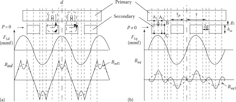
FIGURE 10.2 L-RSM with segmented secondary (a) in axis d and (b) in axis q.

Solving for P, we get

P = τ π \cdot g 1 \cdot F 1 q m \cdot sin π 2 \cdot τ p τ h s s g 2 + τ p 2 π \cdot g 1 (10.6)

$P = \frac{\frac{τ}{π \cdot g_{1}} \cdot F_{1 q m} \cdot \sin \frac{π}{2} \cdot \frac{τ_{p}}{τ}}{\frac{h_{s s}}{g_{2}} + \frac{τ_{p}}{2 π \cdot g_{1}}} (10.6)$

Finally, we get approximately [2]

K d m 1 \approx τ p τ - 1 π sin π \cdot τ p τ (10.7)

$K_{d m 1} \approx \frac{τ_{p}}{τ} - \frac{1}{π} \sin π \cdot \frac{τ_{p}}{τ} (10.7)$

k q m 1 \approx τ p τ + 1 π sin π τ p τ - 4 P π F 1 q m sin π 2 τ p τ (10.8)

$k_{q m 1} \approx \frac{τ_{p}}{τ} + \frac{1}{π} \sin π \frac{τ_{p}}{τ} - \frac{4 P}{π F_{1 q m}} \sin \frac{π}{2} \frac{τ_{p}}{τ} (10.8)$

with τ = 0.24 m, g₁ = 10 mm, 2g₂ = 40 mm, τ_p/τ = (τ − 2g₂)/x = 200/240 = 0.833, we obtain k_dm₁ = 0.673 and k_qm₁ ≈ 0.1 (h_ss = 40 mm).

Now the ratio L_dm/L_qm = 6.73 but the difference L_dm − L_qm = 0.573• L_m, 24% above the 0.46 • L_m for the standard (continuous) secondary. So the thrust for given stator mmf and power angle of the segmented secondary L-RSM will be 20% larger and the power factor notably larger in comparison with the standard (continuous) salient-pole-laminated secondary L-RSM, and again, the weight of the secondary laminations will be notably smaller (less than 50%) in comparison with the continuous variable reluctance secondary.

10.3 L_dm, L_qm (Magnetization) Inductances in Multiple Flux Barrier Secondary L-RSM

Figure 10.1b presents a MFB secondary, mainly feasible in low-speed short travel industrial applications of L-RSM. An analytical approach to calculate the magnetization inductance is given in [3–5] for rotary RSM. In principle, the airgap flux density produced by the primary mmf looks like that in Figure 10.3, if we neglect the primary slot openings.

It should be noticed that the airgap flux density in axis d has space harmonics related to the number of secondary flux barriers per pole (five in Figure 10.3a). In axis q, the airgap flux density crosses zero a few times per pole (it did two times per pole for the segmented secondary (Figure 10.2)). This multiple zero crossing produces increased space harmonics, but also it reduces the fundamental airgap flux density B_aq₁. In Figure 10.3b, zero slot openings in the stator have been considered. In reality, the open slot openings restrict the number of zero crossings per pole of B_aq unless (b₁, b₂) > b_S₁. Mainly for q₁ > 2, 3 slots per pole per phase in the primary and five flux barriers (open slots) per pole in the secondary, the previous condition may be approached.

Images

FIGURE 10.3 Qualitative airgap flux-density variation for MFB secondary L-RSM (a) in axis d and (b) in axis q.

But for low airgap, low pole pitch, semiclosed primary slots, multiple zero crossing of q axis airgap flux density is feasible without increasing too much the slot leakage inductance of primary. This is why for large airgap L-RSM the MFB secondary does not seem practical, besides the higher cost of its manufacturing. For practical designs, 2D FEM (at least) or multiple magnetic circuit model [3] should be used to calculate L_dm and L_qm in MFB secondary. The axially laminated anisotropic (ALA) secondary is just a high number MFB case.

To a first approximation, L_dm may be calculated with (10.7) for τ = 2(b_t₁ + b_t₂ + b_t₃) and L_qm with the same formula but

L q m L d m \approx 4 π k C g 1 k C g 1 + b 2 + b 1 + b 0 / 2 \cdot (1 + k f r i n g e) (10.9)

$\frac{L_{q m}}{L_{d m}} \approx \frac{4}{π} \frac{k_{C} g_{1}}{k_{C g 1} + b_{2} + b_{1} + b_{0} / 2} \cdot (1 + k_{f r i n g e}) (10.9)$

k_fringe depends on the number of flux barriers per pole, airgap to primary slot opening, q₁–slots/pole/phase, etc. [5]. 2(3)D FEM produces more realistic results [6].

10.4 Reduction Of Thrust Pulsations

L-RSM with all these secondary topologies presented in previous paragraphs shows notable thrust pulsations. The τ_p/τ ratio may be optimized to reduce thrust pulsations without severe average thrust reduction. For the MFB secondary, further reduction of thrust pulsations may be obtained by the so-called reluctance equalization design (Figure 10.4) [7].

Images

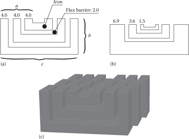
FIGURE 10.4 MFB design (a) conventional, (b) reluctance equalization, and (c) segmented skewing. (After Masayuki. S. et al., Thrust ripple improvement of linear synchronous motor with segmented mover construction, Record of LDIA-2001, Nagano, Japan, pp. 451–455, 2001.)

But still, the main means to reduce thrust pulsations is skewing, segmented skewing in particular (Figure 10.4c). A thrust ripple of only 10.9% is obtained with 5/4 stator slots long three segments skewing (6 slots per primary pole), with reluctance equalization [7] (Figure 10.5).

Typical k_dm₁ and k_qm₁ approximate values for an axially laminated secondary (with many laminations and insulation layers per pole) are given in Figure 10.6 versus pole pitch τ and for a few small airgap values, which are typical for short travel, low-speed, industrial applications.

Images

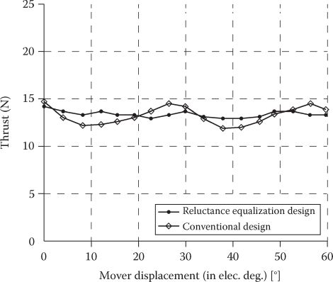
FIGURE 10.5 Thrust ripple with segmented (3/4) slot pitch skewing. (After Boldea, I., Reluctance Synchronous Machines and Drives, Clarendon Press, Oxford, U.K., 1996.)

Images

FIGURE 10.6 k_dm₁ = L_dm/L_m, (a), k_qm₁ = L_qm/L_m, (b) or a multiple lamination insulation layer ALA secondary, (c). (After Boldea, I., Reluctance Synchronous Machines and Drives, Clarendon Press, Oxford, U.K., 1996.)

It may be seen that even at τ = 50 mm and g = 1 mm, k_dm₁=0.95 and k_qm₁ = 0.2; so a good saliency is obtained: L_dm/L_qm = k_dm₁/k_qm₁ = 0.95/0.2 = 4.75 (magnetic saturation was ignored). As the expressions of primary leakage inductance L_sl and resistance R_S per phase are similar to those for LIMs, we skip their derivation here to investigate the dq model of L-RSM.

10.5 dq (Space Phasor) Model of L-RSM

As no dynamic or static longitudinal end effects have been considered—due to large enough number of primary poles (2p ≥ 8)—the dq (space phasor) model of rotary RSM may be adopted here. For mini L-RSM, with 2p = 2,4, 2(3)D FEM should be used to capture the total thrust, normal force, self and mutual phase inductances, etc. The asymmetry of inductances may be alleviated by using a two-phase (dq) primary winding.

The space phasor dq model of L-RSM in secondary (stationary) coordinates is thus

I ¯ S R S - V ¯ ¯ ¯ S = - d Ψ ¯ ¯ ¯ S d t - j ω r Ψ ¯ ¯ ¯ S; ω r = - π τ U (primary as mover) (10.10)

${\bar{I}}_{S} R_{S} - {\bar{V}}_{S} = - \frac{d {\bar{Ψ}}_{S}}{d t} - j ω_{r} {\bar{Ψ}}_{S}; ω_{r} = - \frac{π}{τ} U (primary as mover) (10.10)$

Ψ ¯ ¯ ¯ S = L d I d + j L q I q; I ¯ S = I d + j I q; V ¯ ¯ ¯ S = V d + j V q (10.11)

${\bar{Ψ}}_{S} = L_{d} I_{d} + j L_{q} I_{q}; {\bar{I}}_{S} = I_{d} + j I_{q}; {\bar{V}}_{S} = V_{d} + j V_{q} (10.11)$

L d = L S l + L d m; L q = L S l + L q m (10.12)

$L_{d} = L_{S l} + L_{d m}; L_{q} = L_{S l} + L_{q m} (10.12)$

F x = 3 2 \cdot π τ Real (j ψ ¯ ¯ S \cdot I ¯ * S) = 3 2 π τ \cdot (L d - L q) \cdot I d \cdot I q (10.13)

$F_{x} = \frac{3}{2} \cdot \frac{π}{τ} Real (j {\bar{ψ}}_{S} \cdot {\bar{I}}_{S}^{*}) = \frac{3}{2} \frac{π}{τ} \cdot (L_{d} - L_{q}) \cdot I_{d} \cdot I_{q} (10.13)$

F n = 3 2 \partial ( L d m I 2 d + L q m I 2 q ) \partial g 1 (10.14)

$F_{n} = \frac{3}{2} \frac{\partial (L_{d m} I_{d}^{2} + L_{q m} I_{q}^{2})}{\partial g_{1}} (10.14)$

For steady state d/dt=0, in secondary coordinates (the primary is the mover), and thus the space phasor (vector) diagram of L-RSM is as shown in Figure 10.7. All variables are basically dc in Figure 10.7.

Images

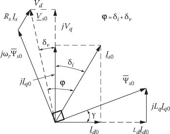
FIGURE 10.7 The space-phasor (dq) model of L-RSM in steady-state and stationary coordinates.

From Figure 10.7,

I S cos φ 1 = I q 0 cos δ v - I d 0 sin δ v; V S 0 = V 2 - \sqrt I d 0 ω r L d = V S 0 cos δ v - I q 0 R S I q 0 ω r L q = V S 0 Sin δ v + I d 0 R S (10.15)

$\begin{array}{l} I_{S} \cos φ_{1} = I_{q 0} \cos δ_{v} - I_{d 0} \sin δ_{v}; V_{S 0} = V \sqrt{2} \\ I_{d 0} ω_{r} L_{d} = V_{S 0} \cos δ_{v} - I_{q 0} R_{S} \\ I_{q 0} ω_{r} L_{q} = V_{S 0} {Sinδ}_{v} + I_{d 0} R_{S} \end{array} (10.15)$

V is the RMS value of phase voltage.

Consequently I_d₀ and I_q₀ are

I d 0 = V S ( ω r L q cos δ v - R S sin δ v ) R 2 S + ω 2 r L d L q I q 0 = V S ( ω r L d sin δ v + R S cos δ v ) R 2 S + ω 2 r L d L q (10.16)

$\begin{matrix} I_{d 0} = \frac{V_{S} (ω_{r} L_{q} \cos δ_{v} - R_{S} \sin δ_{v})}{R_{S}^{2} + ω_{r}^{2} L_{d} L_{q}} \\ I_{q 0} = \frac{V_{S} (ω_{r} L_{d} {sinδ}_{v} + R_{S} \cos δ_{v})}{R_{S}^{2} + ω_{r}^{2} L_{d} L_{q}} \end{matrix} (10.16)$

The electromagnetic (mechanical) power P_m is

P m = F x U = 3 4 V 2 S ( ω r L d - L q ) ( R 2 S + ω 2 r L d L q ) 2 \cdot [(ω 2 r L d L q - R 2 S) sin 2 δ v + R S (ω r L d + ω r L q) cos δ v - R s (ω r L q)] (10.17)

$\begin{array}{l} P_{m} = F_{x} U = \frac{3}{4} \frac{V_{S}^{2} (ω_{r} L_{d} - L_{q})}{{(R_{S}^{2} + ω_{r}^{2} L_{d} L_{q})}^{2}} \\ \begin{array}{l} \cdot [(ω_{r}^{2} L_{d} L_{q} - R_{S}^{2}) \sin 2 δ_{v} + R_{S} (ω_{r} L_{d} + ω_{r} L_{q}) \cos δ_{v} - R_{s} (ω_{r} L_{q})] \end{array} \end{array} (10.17)$

Considering the winding and core (iron) losses, the efficiency and power factor η and cos φ are

η = P m P m + 3 / 2 ( I 2 d 0 + I 2 q 0 ) R s + p i r o n; I S 0 = I 2 d 0 + I 2 q 0 - - - - - - - \sqrt (10.18)

$η= \frac{P_{m}}{P_{m} + 3 / 2 (I_{d 0}^{2} + I_{q 0}^{2}) R_{s} + p_{i r o n}}; I_{S 0} = \sqrt{I_{d 0}^{2} + I_{q 0}^{2}} (10.18)$

cos φ = P m η ( 3 / 2 ) V S 0 I S 0 (10.19)

$\cos φ= \frac{P_{m}}{η (3 / 2) V_{S 0} I_{S 0}} (10.19)$

Neglecting all losses, the maximum ideal power factor cos φ_i_max is

cos φ i max \approx L d - L q L d + L q (10.20)

$\cos φ_{i \max} \approx \frac{L_{d} - L_{q}}{L_{d} + L_{q}} (10.20)$

Note: For LIMs (with no longitudinal end effect), the same formula is valid but L_q → L_S (no load inductance) and L_q → L_Sc (short-circuit inductance).

As it will be demonstrated later, low-speed (low-power) applications of L-RSM may show better power factor and efficiency than LIMs, and thus, lower kVA in the PWM inverter is needed. Including the machine losses would raise the ideal maximum power factor in motoring and will reduce it in generating, as expected.

A typical qualitative variation of propulsion force F_x, attraction force F_n, η, cos φ is shown in Figure 10.8, for given voltage V_S0 and speed U(ω_r) = 90 m/s, for a segmented secondary L-RSM with g₁ = 10 mm airgap.

Images

FIGURE 10.8 Typical steady-state performance on a high-speed L-RSM with segmented (laminated) secondary (track): (a) thrust and normal force and (b) η and cos φ.

A few remarks may be made at this point:

The efficiency is larger (above 90%) over a wide range of power angle (loads).
The power factor for rated thrust may be around 0.5, which is low, but L-RSM provides at least an 8/1 larger normal force than thrust and thus may serve for integrated propulsion–levitation in MAGLEVs (a_max ≈ 1.25 m/s²), if the L-RSM primary represents 12.5% of vehicle weight: this seems feasible as L-RSM is simpler and lighter than H-LSM. However, the low power factor implies a heavier and costlier PWM converter; today’s forced cooled inverters may show less than 1 kg/1 kVA specific weight, which may render the system overall competitive.
The vector control of L-RSM may provide both levitation and propulsion control for a multiple module primary on each vehicle. Propulsion control may be coordinated between units, while vehicle levitation (via flux) control may be robust and decentralized when a secondary and tertiary mechanical suspension are added to the bogie and, respectively, to the cabin. We should remember that even in active guideway dc-excited LSMs for propulsion and suspension systems, power factor per activated section is around 0.6; only H-LSM may show a power factor around (above) 0.8, thus saving weight (and cost) in the PWM converters on board, at the expense of heavier primary of H-LSM on board of vehicle.

10.6 Steady-State Characteristics For Vector Control Strategies

L-RSMs are always supplied from PWM voltage source inverters. Consequently, vector (or direct thrust and flux [DTFC]) control may be applied by using the space phasor (dq) model.

Three main vector control strategies are investigated here:

Constant I_d control
Constant a = I_d/I_q control
Primary flux and thrust control

The L-RSM equivalent circuits (based on (10.10) through (10.14)), for transients in d and q axes, are shown in Figure 10.9.

From (10.10) to (10.13), after I_q elimination,

V 2 S = (R 2 S + ω 2 r L 2 d) I 2 d + (R 2 S + ω 2 r L 2 q) [2 F x τ 3 π ( L d - L q ) I d] 2 - 4 R S ω r τ F x 3 π (10.21)

$V_{S}^{2} = (R_{S}^{2} + ω_{r}^{2} L_{d}^{2}) I_{d}^{2} + (R_{S}^{2} + ω_{r}^{2} L_{q}^{2}) {[\frac{2 F_{x} τ}{3 π (L_{d} - L_{q}) I_{d}}]}^{2} - \frac{4 R_{S} ω_{r} τ F_{x}}{3 π} (10.21)$

Images

FIGURE 10.9 dq axis model equivalent circuit of L-RSM: R_dm, R_qm are core loss resistances, R_suspension is the vertical motion power loss resistance.

with I_d=const., a mild (dc series motor)-type thrust/speed curve (F_x/ω_r), ω_r=π• U/τ, is obtained; the no load (F_x=0) speed U₀ is

U 0 = τ ω r π = τ V 2 S - R S I 2 d - - - - - - - - - \sqrt π L d I d; I q = 2 3 π τ F x ( L d - L q ) I d (10.22)

$U_{0} = τ \frac{ω_{r}}{π} = τ \frac{\sqrt{V_{S}^{2} - R_{S} I_{d}^{2}}}{π L_{d} I_{d}}; I_{q} = \frac{2}{3 π} \frac{τ F_{x}}{(L_{d} - L_{q}) I_{d}} (10.22)$

with I_d=const. and constant airgap g₁, the normal force varies with thrust. The total airgap flux is directly related to normal force:

F n \approx - 1 g 1 (L 2 d m I 2 d + L 2 q m I 2 q) 3 2 (10.23)

$F_{n} \approx - \frac{1}{g_{1}} (L_{d m}^{2} I_{d}^{2} + L_{q m}^{2} I_{q}^{2}) \frac{3}{2} (10.23)$

So even with I_d=const. and constant g₁ (airgap), the normal force increases with thrust (Figure 10.10a). Also F_n is not related directly to speed (10.22) if I_d, I_q control is performed.

For I_d/I_q=α, the stator flux λ_S is

λ S = (L d I d) 2 + (L q I q) 2 - - - - - - - - - - - - - - \sqrt = I d L 2 d + (L 2 q / α 2) - - - - - - - - - - - \sqrt (10.24)

$λ_{S} = \sqrt{{(L_{d} I_{d})}^{2} + {(L_{q} I_{q})}^{2}} = I_{d} \sqrt{L_{d}^{2} + (L_{q}^{2} / α^{2})} (10.24)$

F x = 3 2 π τ (L d - L q) λ 2 S α L 2 d + ( L 2 q / α 2 ) (10.25)

$F_{x} = \frac{3}{2} \frac{π}{τ} (L_{d} - L_{q}) \frac{λ_{S}^{2} α}{L_{d}^{2} + (L_{q}^{2} / α^{2})} (10.25)$

Images

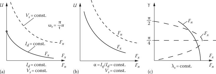
FIGURE 10.10 Three typical ways for vector control: steady-state characteristics; (a) I_d = const., V_S=const., (b) α = I_d/I_q = const., V_S=const., and (c) λ_S=const.

For given voltage V_S ≈ ω_rλ_S, λ_S is given and thus the maximum thrust F_x_max/stator flux λ_S is obtained for α=L_d/L_q:

F x max = 3 π 4 τ ( L d - L q ) L d L q λ 2 S (10.26)

$F_{x \max} = \frac{3 π}{4 τ} \frac{(L_{d} - L_{q})}{L_{d} L_{q}} λ_{S}^{2} (10.26)$

The normal force is

F n = - 3 2 1 g 1 λ 2 S ( L d m + L q m α 2 ) L 2 d + ( L 2 d / α 2 ) (10.27)

$F_{n} = - \frac{3}{2} \frac{1}{g_{1}} \frac{λ_{S}^{2} (L_{d m} + L_{q m} α^{2})}{L_{d}^{2} + (L_{d}^{2} / α^{2})} (10.27)$

Again, where a varies for constant V_S, when speed decreases, λ_S decreases, and thus both F_x and F_n decrease. Care must be exercised for noise and vibration variations (due to normal force) with thrust control. It is also feasible to directly control the DTFC.

In general, primary flux X_S control will take care of airgap (levitation) control (or will maintain λ_S ≈ constant to keep the normal force within bounds), and the flux angle γ control will do thrust control:

cos γ = L d \cdot I d λ S; sin γ = L q \cdot I q λ S (10.28)

$\cos γ = \frac{L_{d} \cdot I_{d}}{λ_{S}}; \sin γ = \frac{L_{q} \cdot I_{q}}{λ_{S}} (10.28)$

F x = 3 4 π τ (L d - L q) λ 2 S L d \cdot L q sin 2 γ; - π 4 \leq γ \leq π 4 F n \approx - 3 2 1 g 1 λ 2 S (L d m L 2 d cos 2 γ + L q m L 2 q sin 2 γ) (10.29)

$\begin{array}{l} F_{x} = \frac{3}{4} \frac{π}{τ} (L_{d} - L_{q}) \frac{λ_{S}^{2}}{L_{d} \cdot L_{q}} \sin 2 γ; - \frac{π}{4} \leq γ \leq \frac{π}{4} \\ F_{n} \approx - \frac{3}{2} \frac{1}{g_{1}} λ_{S}^{2} (\frac{L_{d m}}{L_{d}^{2}} \cos^{2} γ+ \frac{L_{q m}}{L_{q}^{2}} \sin^{2} γ) \end{array} (10.29)$

The maximum thrust is obtained again for γ = π/4 and thus L_d • I_d=L_q • I_q, but now the thrust may be controlled through γ and normal force by λ_S; though the two functions are not fully decoupled, as seen in (10.29), F_n is less dependent on γ than F_x. So, if F_x and F_n are regulated in different frequency bands, their simultaneous control seems feasible.

10.7 Design Methodology for low Speed by Example

Let us consider the design of a short travel (l_t ≈ 2 m) L-RSM that is able to produce a peak thrust F_x_max = 1.6 kN from zero to the maximum speed U_max = 2 m/s for a short duty cycle (20%). The continuous duty thrust is F_x = 0.8 kN. An airgap g = 0.5 mm is mechanically feasible; the ALA secondary (track) is placed above the primary (mover); the latter is fed by a three-phase ac power flexible cable.

Solution

(a) Primary geometry and maximum mmf per slot

First, a reasonable saliency ratio L_dm/L_qm has to be secured. Consequently, a high ratio between the pole pitch T and airgap is chosen: τ = 200; g₁ = 200 • 5 • 10⁻³ = 0.1 m. For U_max = 2 m/s, it would mean a frequency f_1max = U_max/2τ, the unsaturated k_dm₁ = 0.97; with the leakage inductance L_ls=0.17 L_m, L_dm/L_qm = 15/1, and a magnetic saturation coefficient k_Sd=0.3, the ratio L_d/L_q becomes

L d L q = 0.97 ( L m / ( 1 + k S d ) ) + L l S 0.97 ( L m / 20 ) + L l S = ( 0.97 / 1.3 ) + 0.07 ( 0.97 / 15 ) + 0.07 = 6.06 (10.30)

$\frac{L_{d}}{L_{q}} = \frac{0.97 (L_{m} / (1 + k_{S d})) + L_{l S}}{0.97 (L_{m} / 20) + L_{l S}} = \frac{(0.97 / 1.3) + 0.07}{(0.97 / 15) + 0.07} = 6.06 (10.30)$

The maximum thrust is considered to be obtained in conditions of maximum thrust per flux: for L_dI_d=L_qI_q. If the d axis airgap flux density produced by I_d is B_d₁_p, the resultant airgap flux density B_g₁_k for maximum thrust

B d 1 p = B 1 g k 1 + ( L d / L q ) 2 ( L q m ( 1 + k S d ) / L d m ) 2 - - - - - - - - - - - - - - - - - - - - - - - - - - - \sqrt (10.31)

$B_{d 1 p} = \frac{B_{1 g k}}{\sqrt{1 + {(L_{d} / L_{q})}^{2} {(L_{q m} (1 + k_{S d}) / L_{d m})}^{2}}} (10.31)$

Making sure that B_g₁_k is within reasonable limits—B_g₁_k=0.75 T—B_d₁_p is from (10.31):

B d 1 p e a k = 0.75 1 + 6.06 2 \cdot ( 1.3 / 15 ) 2 - - - - - - - - - - - - - - - - \sqrt = 0.664 T (10.32)

$B_{d 1 p e a k} = \frac{0.75}{\sqrt{1 + {6.06}^{2} \cdot {(1.3 / 15)}^{2}}} = 0.664 T (10.32)$

On the other hand, this airgap flux-density component B_d_1peak is related to the I_d component of phase current by

B d 1 p = μ 0 \cdot 3 2 - \sqrt \cdot k W 1 W 1 \cdot I d p e a k \cdot k d m 1 π \cdot k C ( 1 + k S d ) g 1 \cdot p 1 (10.33)

$B_{d 1 p} = \frac{μ_{0} \cdot 3 \sqrt{2} \cdot k_{W 1} W_{1} \cdot I_{d p e a k} \cdot k_{d m 1}}{π \cdot k_{C} (1 + k_{S d}) g_{1} \cdot p_{1}} (10.33)$

where k_C ≈ 1.3 (Carter coefficient), p₁ – pole pairs, W₁ – turns per phase, kW1=0.925(q1=2,y/τ=5/6) $k_{W_{1}} = 0.925 (q_{1} = 2, y / τ=5/6)$ .

From (10.33), we may calculate the phase d axis current component mmf, for peak thrust, W₁I_d_peak, as

W 1 I d peak = 0.664 \times π \times 1 .3 \times 1 .3 \times 0.5 \times 10 - 3 \times p 3 2 - \sqrt \times 1.256 \times 10 - 6 \times 0.925 = 358.5 \times p 1 (10.34)

$W_{1} I_{d peak} = \frac{0.664 \times π \times 1 .3 \times 1 .3 \times 0.5 \times 10^{- 3} \times p}{3 \sqrt{2} \times 1.256 \times 10^{- 6} \times 0.925} = 358.5 \times p_{1} (10.34)$

Note: I_df and I_qf refer to RMS phase current components.

The q axis mmf peak value W₁I_q_peak is

W 1 I d peak = W 1 I d peak \cdot L d L q = 358.5 \times 6.06 = 2172 \times p 1 A \cdot turns (10.35)

$W_{1} I_{d peak} = W_{1} I_{d peak} \cdot \frac{L_{d}}{L_{q}} = 358.5 \times 6.06 = 2172 \times p_{1} A \cdot turns (10.35)$

The peak thrust F_x_peak is

F x peak = 3 2 π τ L m (k d m 1 1 + k S d - k q m 1 k q m 1) (I d f p 2 - \sqrt) (I q f p 2 - \sqrt) (10.36)

$F_{x peak} = \frac{3}{2} \frac{π}{τ} L_{m} (\frac{k_{d m 1}}{1 + k_{S d}} - \frac{k_{q m 1}}{k_{q m 1}}) (I_{d f p} \sqrt{2}) (I_{q f p} \sqrt{2}) (10.36)$

with k_dm₁/k_qm₁ = 15, k_dm₁ = 0.97, 1+k_Sd = 1.3, τ = 0.1 m and

L m = 6 μ 0 \cdot ( k W 1 \cdot W 1 ) 2 \cdot τ \cdot L π 2 \cdot k C \cdot g 1 \cdot p 1 (10.37)

$L_{m} = \frac{6 μ_{0} \cdot {(k_{W_{1}} \cdot W_{1})}^{2} \cdot τ \cdot L}{π^{2} \cdot k_{C} \cdot g_{1} \cdot p_{1}} (10.37)$

where again, τ = 0.1 m, kW1=0.925 $k_{W_{1}} = 0.925$ , k_C = 1.3, g₁ = 0.5 mm, F_x_peak = 1.6 kN and we find

1600 = 16 \times 1.256 \times 10 - 6 \times 0.925 2 \times 358.5 \times 2172 \times ( p 1 \cdot L ) ( ( 0.97 / 1.3 ) - ( 1 / 15 ) ) π \cdot 1 .3 \times 0 .5 \times 10 - 3 (10.38)

$1600 = \frac{16 \times 1.256 \times 10^{- 6} \times {0.925}^{2} \times 358.5 \times 2172 \times (p_{1} \cdot L) ((0.97 / 1.3) - (1 / 15))}{π \cdot 1 .3 \times 0 .5 \times 10^{- 3}} (10.38)$

so p₁ • L = 0.359 m. It is now time to choose the number of poles, say 2p = 6, and thus, the stack width L=0.359/3 = 0.12 m. The peak thrust density f_x_p is

f x p = F x max 2 p τ L = 1600 2 \times 3 \times 0.1 \times 0.12 = 2.22 \times 104 N/m 2 = 2.22 N/cm 2 (10.39)

$f_{x p} = \frac{F_{x \max}}{2 p τ L} = \frac{1600}{2 \times 3 \times 0.1 \times 0.12} = 2.22 \times 10^{4} {N/m}^{2} = 2.22 {N/cm}^{2} (10.39)$

This may be termed as a good value (even for a linear PM synchronous motor of similar size and output).

(b) Primary slot design (Figure 10.11)

With q₁ = 2 slots/pole/phase, the peak value of slot mmf (RMS value), n₁I_1p, is

n 1 \cdot I 1 peak = W 1 \cdot I 1 p p \cdot q = 358.5 \cdot p 1 \cdot 1 + 6.06 2 - - - - - - - \sqrt p 1 \cdot 2 = 1100.945 A \cdot turns/slot (10.40)

$n_{1} \cdot I_{1 peak} = \frac{W_{1} \cdot I_{1 p}}{p \cdot q} = \frac{358.5 \cdot p_{1} \cdot \sqrt{1 + {6.06}^{2}}}{p_{1} \cdot 2} = 1100.945 A \cdot turns/slot (10.40)$

n₁ is the turns per slot (two coils per slot)

For a duty cycle of 20%, the average peak slot mmf (RMS) n₁I_avp is

n 1 I a v p = n 1 I p e a k 0.2 - - - \sqrt = 1100.745 \times 0.2 - - - \sqrt = 492 A \cdot turns (10.41)

$n_{1} I_{a v p} = n_{1} I_{p e a k} \sqrt{0.2} = 1100.745 \times \sqrt{0.2} = 492 A \cdot turns (10.41)$

The slot pitch τ_s is

τ S = τ 2 \times 3 = 100 6 = 16.66 mm (10.42)

$τ_{S} = \frac{τ}{2 \times 3} = \frac{100}{6} = 16.66 mm (10.42)$

With teeth width b_t₁ = τ_s/2 ≈ 8 mm. So the slot depth h_s is

h S = A s l o t b b s 1 = 307.5 116.66 - 8 = 35.5 mm (10.43)

$h_{S} = \frac{A_{s l o t}}{b_{b s 1}} = \frac{307.5}{116.66 - 8} = 35.5 mm (10.43)$

The primary stack thickness h_c₁ is

h c 1 = B g 1 p B c p . τ π = 0.75 1.5 \times 0.1 π = 0.016 m (10.44)

$h_{c 1} = \frac{B_{g 1 p}}{B_{c p}} . \frac{τ}{π} = \frac{0.75}{1.5} \times \frac{0.1}{π} = 0.016 m (10.44)$

Images

FIGURE 10.11 Primary slotting geometry (a) and ALA secondary topology (b) with 2p = 6, but for a double-layer chorded (y/τ = 5/6) coils.

The end slots are half field, and thus, the machine has (2p + 1) • q • m − 1 = 41 slots and 42 teeth. The total length of primary L_p is

L p \approx 41 \times τ S + τ S = 42 \times τ S \approx 700 mm =0 .7 m (10.45)

$L_{p} \approx 41 \times τ_{S} + τ_{S} = 42 \times τ_{S} \approx 700 mm =0 .7 m (10.45)$

We may now calculate the circuit model parameters (Figure 10.9).

Let us notice that the number of turns/phase W₁ is not yet calculated, for a given voltage.

The phase resistance R_S is

R S = 2 \cdot δ C o \cdot ( L + 0.01 + 1.5 y ) \cdot W 2 1 W 1 I a v p J a v c o = 2 \cdot 2.3 \cdot 10 - 8 ( 0.12 + 0.01 + 1.5 \cdot ( 5 / 6 ) \cdot 0.1 ) 6 \times 492 \times 4 \times 106 \cdot W 21 = 1.589 \times 10 - 5 \cdot W 21 (10.46)

$\begin{array}{l} R_{S} = 2 \cdot δ_{C o} \cdot \frac{(L + 0.01 + 1.5 y) \cdot W_{1}^{2}}{W_{1} I_{a v p}} J_{a v c o} \\ = 2 \cdot 2.3 \cdot 10^{- 8} \frac{(0.12 + 0.01 + 1.5 \cdot (5 / 6) \cdot 0.1)}{6 \times 492} \times 4 \times 10^{6} \cdot W_{1}^{2} = 1.589 \times 10^{- 5} \cdot W_{1}^{2} \end{array} (10.46)$

n 1 \cdot p 1 \cdot q = W 1; W 1 \cdot I a v p = p 1 \cdot q \cdot n 1 I a v p = 3 \times 2 \times 492 (10.47)

$n_{1} \cdot p_{1} \cdot q = W_{1}; W_{1} \cdot I_{a v p} = p_{1} \cdot q \cdot n_{1} I_{a v p} = 3 \times 2 \times 492 (10.47)$

l C = 2 \cdot (L + 0.01 + 1.5 \cdot y) = 2 \times 0.255 = 0.51 m/turn (10.48)

$l_{C} = 2 \cdot (L + 0.01 + 1.5 \cdot y) = 2 \times 0.255 = 0.51 m/turn (10.48)$

The unsaturated uniform airgap inductance L_m (10.2) is

L m = 6 μ 0 ( k W 1 \cdot W 1 ) 2 \cdot τ \cdot L π 2 p 1 \cdot k C g 1 = 6 \times 1.256 \times 10 - 6 \cdot 0.925 2 \times 0.12 \times 0.1 \times W 2 1 π 2 \cdot 3 \times 1.3 \times 0.5 \times 10 - 3 = 4.239 \times 10 - 6 \cdot W 21 (10.49)

$L_{m} = \frac{6 μ_{0} {(k_{W_{1}} \cdot W_{1})}^{2} \cdot τ \cdot L}{π^{2} p_{1} \cdot k_{C g 1}} = \frac{6 \times 1.256 \times 10^{- 6} \cdot {0.925}^{2} \times 0.12 \times 0.1 \times W_{1}^{2}}{π^{2} \cdot 3 \times 1.3 \times 0.5 \times 10^{- 3}} = 4.239 \times 10^{- 6} \cdot W_{1}^{2} (10.49)$

Consequently

L d m = k d m 1 1 + k S d \cdot L m = 0.97 1.3 \times 4.239 \times 10 - 6 \cdot W 21 = 3.1637 \times 10 - 6 \cdot W 21 (10.50)

$L_{d m} = \frac{k_{d m 1}}{1 + k_{S d}} \cdot L_{m} = \frac{0.97}{1.3} \times 4.239 \times 10^{- 6} \cdot W_{1}^{2} = 3.1637 \times 10^{- 6} \cdot W_{1}^{2} (10.50)$

L q m = k q m 1 k d m 1 \cdot L m = 1 15 \times 4.239 \times 10 - 6 \cdot W 21 = 0.2826 \times 10 - 6 \cdot W 21 (10.51)

$L_{q m} = \frac{k_{q m 1}}{k_{d m 1}} \cdot L_{m} = \frac{1}{15} \times 4.239 \times 10^{- 6} \cdot W_{1}^{2} = 0.2826 \times 10^{- 6} \cdot W_{1}^{2} (10.51)$

The leakage inductance is

L l s = 2 μ 0 p 1 \cdot q W 21 (λ S S \cdot L + λ l \cdot l l c) (10.52)

$L_{l s} = \frac{2 μ_{0}}{p_{1} \cdot q} W_{1}^{2} (λ_{S S} \cdot L + λ_{l} \cdot l_{l c}) (10.52)$

The slot permeance λ_ss is

λ S S = h S 1 3 b S 1 + h S a b S a = 35.5 3 \times 8 + 1 2 + 2 2 + 8 = 2.18 (10.53)

$λ_{S S} = \frac{h_{S 1}}{3 b_{S 1}} + \frac{h_{S a}}{b_{S a}} = \frac{35.5}{3 \times 8} + \frac{1}{2} + \frac{2}{2 + 8} = 2.18 (10.53)$

λ l = 0.3 \cdot q \cdot (3 \cdot β 1 - 1) = 0.3 \times 2 \times (3 \times 5 6 - 1) = 0.9 (10.54)

$λ_{l} = 0.3 \cdot q \cdot (3 \cdot β_{1} - 1) = 0.3 \times 2 \times (\frac{3 \times 5}{6} - 1) = 0.9 (10.54)$

The end connection (side) length

l l C = 0.01 + 1.5 y = 0.01 + 1.5 \times 5 6 0.1 = 0.135 m (10.55)

$l_{l C} = 0.01 + 1.5 y = 0.01 + 1.5 \times \frac{5}{6} 0.1 = 0.135 m (10.55)$

Finally, from (10.52) to (10.55),

L l s = 2 \times 1.256 \times 10 - 6 3 \times 2 \cdot (2.18 \times 0.1 + 0.9 \times 0.135) \cdot W 21 = 0.142 \times 10 - 6 \cdot W 21 (10.56)

$L_{l s} = \frac{2 \times 1.256 \times 10^{- 6}}{3 \times 2} \cdot (2.18 \times 0.1 + 0.9 \times 0.135) \cdot W_{1}^{2} = 0.142 \times 10^{- 6} \cdot W_{1}^{2} (10.56)$

As can be seen, the leakage inductance ratio L_ls/L_m = 0.142/3.1637 = 0.0449; it is smaller than presumed (L_ls/L_m = 0.078), and thus, the design is safe.

The L_d/L_q ratio becomes now

L d L q = ( 0.142 + 3.1637 ) \times 10 - 6 \cdot W 2 1 ( 0.142 + 0.2826 ) \times 10 - 6 \cdot W 2 1 = 7.77 > 6.06 (10.57)

$\frac{L_{d}}{L_{q}} = \frac{(0.142 + 3.1637) \times 10^{- 6} \cdot W_{1}^{2}}{(0.142 + 0.2826) \times 10^{- 6} \cdot W_{1}^{2}} = 7.77 > 6.06 (10.57)$

(d) Turns per phase W₁

Let us consider that we have a V_dc = 500 Vdc power source available for the L-RSM drive. This volt-age should be sufficient to deliver rated thrust, at good efficiency, and the peak (maximum) thrust at maximum speed U_max = 2 m/s.

The RMS phase voltage V_ph_max is

V p h max = 4 k \cdot Vdc π 6 - \sqrt = 4 \times 0.85 \times 500 π 6 - \sqrt \approx 221 V (RMS/phase) (10.58)

$V_{p h \max} = \frac{4 k \cdot Vdc}{π \sqrt{6}} = \frac{4 \times 0.85 \times 500}{π \sqrt{6}} \approx 221 V (RMS/phase) (10.58)$

To yield good performance at rated thrust, we may choose to produce it at maximum power factor, which corresponds to

I q I d = L d L q = - - - - - \sqrt 7.77 - - - - \sqrt = 2.787 (10.59)

$\frac{I_{q}}{I_{d}} = \sqrt{\frac{L_{d}}{L_{q}} =} \sqrt{7.77} = 2.787 (10.59)$

With the same saturation level for maximum and rated thrust, the ratio of d axis mmf for the two forces is simply

F x F x max = (W 1 I d max W 1 I d phase) - 2 \times L d / L q - - - - - \sqrt L d / L q (10.60)

$\frac{F_{x}}{F_{x \max}} = {(\frac{W_{1} I_{d \max}}{W_{1} I_{d phase}})}^{- 2} \times \frac{\sqrt{L_{d} / L_{q}}}{L_{d} / L_{q}} (10.60)$

W 1 I d phase = 3 \times 358.5 \times 800 1600 \times 6.606 2.781 - - - - - - - - - - - - \sqrt = 3 \times 423.26 A \cdot turns (10.61)

$W_{1} I_{d phase} = 3 \times 358.5 \times \sqrt{\frac{800}{1600} \times \frac{6.606}{2.781}} = 3 \times 423.26 A \cdot turns (10.61)$

Consequently

W 1 I q phase = W 1 I d phase \cdot 2.787 = 1121.38 \times 2.787 = 3125.3 A \cdot turns (10.62)

$W_{1} I_{q phase} = W_{1} I_{d phase} \cdot 2.787 = 1121.38 \times 2.787 = 3125.3 A \cdot turns (10.62)$

These are phase mmf RMS values.

Let us now use the space phasor diagram where Vph→VS=Vph2–√,Id phase→Id=Id phase2–√,Iq phase→Iq=Iq phase2–√ $V_{p h} \to V_{S} = V_{p h} \sqrt{2}, I_{d phase} \to I_{d} = I_{d phase} \sqrt{2}, I_{q phase} \to I_{q} = I_{q phase} \sqrt{2}$ to calculate the number of turns per phase W₁:

V d = R S \cdot I d - ω r \cdot L q \cdot I q V q = R S \cdot I q + ω r \cdot L d \cdot I d (10.63)

$\begin{matrix} V_{d} = R_{S} \cdot I_{d} - ω_{r} \cdot L_{q} \cdot I_{q} \\ V_{q} = R_{S} \cdot I_{q} + ω_{r} \cdot L_{d} \cdot I_{d} \end{matrix} (10.63)$

V d phase = V d 2 - \sqrt = 1.589 \times 10 - 5 \cdot W 2 1 I d 2 - \sqrt - 62.8 \times 0.4246 \times 10 - 6 \cdot W 2 1 I q 2 - \sqrt = - 0.0652. W (10.64)

$V_{d phase} = \frac{V_{d}}{\sqrt{2}} = 1.589 \times 10^{- 5} \cdot \frac{W_{1}^{2} I_{d}}{\sqrt{2}} - 62.8 \times 0.4246 \times 10^{- 6} \cdot \frac{W_{1}^{2} I_{q}}{\sqrt{2}} = - 0.0652. W (10.64)$

V q phase = V d 2 - \sqrt = 1.589 \times 10 - 5 \cdot W 21 I q + 62.8 \times 3.305 \times 10 - 6 \cdot W 21 I d = 0.281. W 1 (10.65)

$V_{q phase} = \frac{V_{d}}{\sqrt{2}} = 1.589 \times 10^{- 5} \cdot W_{1}^{2} I_{q} + 62.8 \times 3.305 \times 10^{- 6} \cdot W_{1}^{2} I_{d} = 0.281. W_{1} (10.65)$

V p h = V 2 d phase + V 2 q phase - - - - - - - - - - - - - \sqrt = W 1 0.0652 2 + 0.281 2 - - - - - - - - - - - - - \sqrt = 220 (10.66)

$V_{p h} = \sqrt{V_{d phase}^{2} + V_{q phase}^{2}} = W_{1} \sqrt{{0.0652}^{2} + {0.281}^{2}} = 220 (10.66)$

W 1 = 220 0.2886 = 762 turns/phase (10.67)

$W_{1} = \frac{220}{0.2886} = 762 turns/phase (10.67)$

The number of turns per coil n_c is

n c = n 1 2 = W 1 2 p q = 762 6 \times 2 \approx 63 turns/coil (10.68)

$n_{c} = \frac{n_{1}}{2} = \frac{W_{1}}{2 p q} = \frac{762}{6 \times 2} \approx 63 turns/coil (10.68)$

Now,

I d phase = W 1 I d phase W 1 = 1121.38 756 = 1.4833 A (10.69)

$I_{d phase} = \frac{W_{1} I_{d phase}}{W_{1}} = \frac{1121.38}{756} = 1.4833 A (10.69)$

I q phase = W 1 I q phase W 1 = 3125.3 756 = 4.134 A (10.70)

$I_{q phase} = \frac{W_{1} I_{q phase}}{W_{1}} = \frac{3125.3}{756} = 4.134 A (10.70)$

The phase current (RMS) for rated thrust (F_xn = 800 N) is

I 1 = I 2 d phase + I 2 q phase - - - - - - - - - - - - \sqrt = 1.484 2 + 4.134 2 - - - - - - - - - - - - \sqrt = 4.392 A (10.71)

$I_{1} = \sqrt{I_{d phase}^{2} + I_{q phase}^{2}} = \sqrt{{1.484}^{2} + {4.134}^{2}} = 4.392 A (10.71)$

So the product η_n cos φ_n is

η n cos φ n = F x U max 3 V phase I 1 = 800.2 3.22 \times 4.392 = 0.552 (10.72)

$η_{n} \cos φ_{n} = \frac{F_{x} U_{\max}}{3 V_{phase} I_{1}} = \frac{800.2}{3.22 \times 4.392} = 0.552 (10.72)$

The copper losses p_con are

p c o n = 3 R S \cdot I 21 = 3 \times 4.392 2 \times 1.589 \times 10 - 5 \times 7562 = 525 W (10.73)

$p_{c o n} = 3 R_{S} \cdot I_{1}^{2} = 3 \times {4.392}^{2} \times 1.589 \times 10^{- 5} \times 756^{2} = 525 W (10.73)$

With f₁_n = 10 Hz, core losses may be neglected, and thus, efficiency and power factor at F_xn=800 N and U_max=2 m/s are

η n = 1 1 + p c o n / F x n U max = 0.7529; cos φ n = η n cos φ n η n = 0.552 0.7529 = 0.733 (10.74)

$η_{n} = \frac{1}{1 + p_{c o n} / F_{x n} U_{\max}} = 0.7529; \cos φ_{n} = \frac{η_{n} \cos φ_{n}}{η_{n}} = \frac{0.552}{0.7529} = 0.733 (10.74)$

This is quite good performance at 2 m/s and 1.6 kW of mechanical power.

(e) Verification of peak thrust at maximum speed

As we designed the L-RSM at rated thrust and maximum voltage, a verification of machine capability to produce the maximum thrust at the same (maximum) speed is required. For the purpose, we use again the voltage equations, but now with

W 1 I d peak = 1075.5 A \cdot turns (10.75)

$W_{1} I_{d peak} = 1075.5 A \cdot turns (10.75)$

W 1 I q peak = 1075.5 \times 6.06 = 6453 A \cdot turns (10.76)

$W_{1} I_{q peak} = 1075.5 \times 6.06 = 6453 A \cdot turns (10.76)$

From (10.63),

V d phase = (1.589 \times 10 - 5 \times 1075.5 - 62.8 \times 0.4246 \times 10 - 6 \times 6453) \times 756 = - 117.44 V (10.77)

$V_{d phase} = (1.589 \times 10^{- 5} \times 1075.5 - 62.8 \times 0.4246 \times 10^{- 6} \times 6453) \times 756 = - 117.44 V (10.77)$

V q phase = (1.589 \times 10 - 5 \times 6.453 + 62.8 \times 3.305 \times 10 - 6 \times 1075.5) \times 756 = 246.2 V (10.78)

$V_{q phase} = (1.589 \times 10^{- 5} \times 6.453 + 62.8 \times 3.305 \times 10^{- 6} \times 1075.5) \times 756 = 246.2 V (10.78)$

V phase = 117.4 2 + 246.2 2 - - - - - - - - - - - - \sqrt = 272.84 V (10.79)

$V_{phase} = \sqrt{{117.4}^{2} + {246.2}^{2}} = 272.84 V (10.79)$

Note: As seen from (10.77), the L-RSM is not capable to produce the maximum thrust F_x_max = 2F_xn = 1.6 kN at 2 m/s at 220 V. This simply means that the voltage for rated thrust should be chosen smaller; this would lead to a smaller number of turns per coil and larger current, but same efficiency and power factor. The main drawback of this choice is that the peak kVA of the inverter will end up larger, and so will its cost.

(f) Primary active weight

The primary active weight comprises iron core (G_iron) and copper weight, G_Co:

G C o = 3 W 1 I a v J a v C o \times 2 (L + 0.01 + 1.5 \times 5 6 \times 0.1) \times γ C o = 3.756 \times 492 63 \times 2 \times 4 \times 10 6 \times 2 \times 0.255 \times 8900 \times 10.05 kg (10.80)

$\begin{array}{l} G_{C o} = 3 W_{1} \frac{I_{a v}}{J_{a v C o}} \times 2 (L + 0.01 + 1.5 \times \frac{5}{6} \times 0.1) \times γ_{C o} \\ = 3.756 \times \frac{492}{63 \times 2 \times 4 \times 10^{6}} \times 2 \times 0.255 \times 8900 \times 10.05 kg \end{array} (10.80)$

G i r o n = G t e e t h + G c o r e \approx (43 \times 37.5 \times 10 - 3 \times 8 \times 10 - 3 \times 0.12 + 0.7 \times 0.12 \times 0.016) \times 7600 = 21.98 kg (10.81)

$\begin{array}{l} G_{i r o n} = G_{t e e t h} + G_{c o r e} \approx (43 \times 37.5 \times 10^{- 3} \times 8 \times 10^{- 3} \times 0.12 + 0.7 \times 0.12 \times 0.016) \times 7600 \\ = 21.98 kg \end{array} (10.81)$

So the active weight of primary G_a₁ is

G a 1 = G C o + G i r o n = 10.05 + 21.98 \approx 32 kg (10.82)

$G_{a 1} = G_{C o} + G_{i r o n} = 10.05 + 21.98 \approx 32 kg (10.82)$

The peak thrust/primary weight = 1600/32 ≈ 50 N/kg, which would mean an ideal acceleration of more than 5 g_grav.

10.8 Control of L-RSM

So far we have dealt with the steady-state theory and performance of L-RSM with notable attention to its electromagnetic design. Some main vector control possibilities have been also introduced through their potential characteristics, to assist in the design. Here, we will introduce a rather new vector control scheme for propulsion and the direct thrust and normal force control for integrated propulsion and suspension control.

10.8.1 “Active Flux” Vector Control of L-RSM

The active flux [8] ψad $ψ_{d}^{a}$ is defined as

ψ a d = ψ ¯ ¯ S - L q \cdot I ¯ S = (L d - L q) I q (10.83)

$ψ_{d}^{a} = {\bar{ψ}}_{S} - L_{q} \cdot {\bar{I}}_{S} = (L_{d} - L_{q}) I_{q} (10.83)$

The thrust F_x is thus

F x = 3 2 π τ ψ a d \cdot I q (10.84)

$F_{x} = \frac{3}{2} \frac{π}{τ} ψ_{d}^{a} \cdot I_{q} (10.84)$

The dq model may be written in terms of active flux by replacing ψ¯¯S ${\bar{ψ}}_{S}$ in (10.10) by using (10.81):

I ¯ S \cdot R S - V ¯ ¯ ¯ S = - d ψ a d d t - j ω r \cdot ψ a d - L q d I ¯ S d t - j ω r \cdot L q d I ¯ S d t (10.85)

${\bar{I}}_{S} \cdot R_{S} - {\bar{V}}_{S} = - \frac{d ψ_{d}^{a}}{d t} - j ω_{r} \cdot ψ_{d}^{a} - L_{q} \frac{d {\bar{I}}_{S}}{d t} - j ω_{r} \cdot L_{q} \frac{d {\bar{I}}_{S}}{d t} (10.85)$

So in fact by the active flux concept, we turn the anisotropic (salient pole) machine into an isotropic machine with inductance L_q along both d and q axes.

For a direct vector control scheme, the active flux has to be estimated. It suffices to estimate properly the stator flux ψ¯¯S ${\bar{ψ}}_{S}$ (by a combined voltage and current model) and then use (10.83) to obtain ψad $ψ_{d}^{a}$ (Figure 10.12). As evident from (10.83), the active flux is always aligned to axis d, irrespective of thrust, which means simpler mover position estimation in a sensorless control system.

For very low speeds, including standstill, the same active flux observer may be used but with an additional high-frequency voltage signal injection, which, after filtering, yields the initial mover position (for nonhesitant heavy starting) and the position at better precision for very low speeds. The signal injection position observer part corrects the fundamental one, and then it is made to fade away with increasing speed. For absolute positioning of the mover, either a linear encoder is provided or, at least, certain calibration position information is available.

A typical vector control system is shown in Figure 10.13.

The control scheme in Figure 10.13 is characterized by

Combined PI and sliding mode (robust) active flux and I_q close-loop regulation and a robust PI + SM speed regulator.
The ac voltages are not measured, but a combination of reference voltages V∗a,V∗b,V∗c $V_{a}^{*}, V_{b}^{*}, V_{c}^{*}$ and the dc voltage info is used, instead. The active flux observer is provided with PLL position and speed estimators (Figure 10.12).
An emf compensation may be added to yield V∗d $V_{d}^{*}$ and V∗q $V_{q}^{*}$ , but since active flux is regulated and the regulators are robust, such an addition may not be necessary.

Images

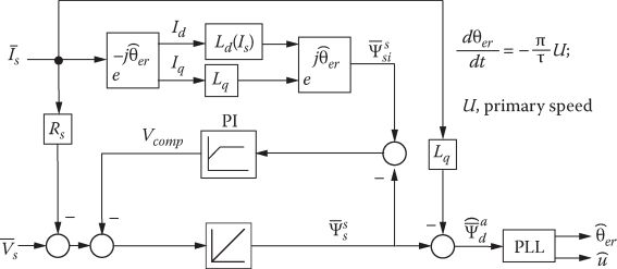
FIGURE 10.12 Generic active flux observer with PLL mover position and speed estimator.

Images

FIGURE 10.13 Generic active flux vector speed sensorless control of L-RSM.

10.8.2 Direct Thrust and Normal Force (Levitation) Control

When integrated propulsion–levitation control is targeted (MAGLEVs), the control is more elaborated but the mover position and speed estimation are again necessary.

In this case, however, the thrust as well as the normal force have to be estimated:

F ⌢ x = 3 2 π τ Real (j ψ ⌢ S \cdot I ⌢ * S) = 3 2 π τ (ψ ⌢ α \cdot I β - ψ ⌢ β \cdot I) (10.86)

${\overset{⌢}{F}}_{x} = \frac{3}{2} \frac{π}{τ} Real (j {\overset{⌢}{ψ}}_{S} \cdot {\overset{⌢}{I}}_{S}^{*}) = \frac{3}{2} \frac{π}{τ} ({\overset{⌢}{ψ}}_{α} \cdot I_{β} - {\overset{⌢}{ψ}}_{β} \cdot I_{}) (10.86)$

F n \approx - 3 2 1 g 1 (L ⌢ d m \cdot I 2 d + L ⌢ q m \cdot I 2 q) (10.87)

$F_{n} \approx - \frac{3}{2} \frac{1}{g_{1}} ({\overset{⌢}{L}}_{d m} \cdot I_{d}^{2} + {\overset{⌢}{L}}_{q m} \cdot I_{q}^{2}) (10.87)$

From the active flux observer (Figure 10.12), we may further estimate

(L ⌢ d m - L ⌢ q m) \cdot I d = ∣ ∣ ψ ⌢ a d ∣ ∣ (10.88)

$({\overset{⌢}{L}}_{d m} - {\overset{⌢}{L}}_{q m}) \cdot I_{d} = | {\overset{⌢}{ψ}}_{d}^{a} | (10.88)$

In a first approximation, L⌢dm/L⌢qm≈ ${\overset{⌢}{L}}_{d m} / {\overset{⌢}{L}}_{q m} \approx$ ≈ constant and known from design.

Consequently, both L⌢dm ${\overset{⌢}{L}}_{d m}$ and L⌢qm ${\overset{⌢}{L}}_{q m}$ (magnetization inductances) may be estimated. The airgap may be measured by a dedicated sensor or (at least for redundancy) it may be estimated, as L⌢dm ${\overset{⌢}{L}}_{d m}$ is (for constant saturation) inversely proportional to airgap.

The currents I_d and I_q are available in the active flux observer and so are the mover position and speed estimations. It is inferred here that a robust (PI+SM) airgap control is feasible for a multiunit vehicle.

A potential thrust and airgap via flux control (DTFC) for L-RSM for integrated propulsion–levitation are introduced in Figure 10.14.

There are three regulators in row, for airgap normal force and active flux control; as they are all robust, the numerous nonlinearities of L-RSM and the track irregularities may be handled even in presence of normal force perturbations from other units on board of vehicle.
The transformation of coordinates is skipped for DTFC, but a table of switching sequences in the inverter is defined as the angles of both stator flux ψ¯¯S−θ⌢ψ¯¯S ${\bar{ψ}}_{S} - {\overset{⌢}{θ}}_{{\bar{ψ}}_{S}}$ and of mover position (axis d) ψ¯¯ad−θ⌢ψ¯¯ad ${\bar{ψ}}_{d}^{a} - {\overset{⌢}{θ}}_{{\bar{ψ}}_{d}^{a}}$ are available from the active flux extended observer.
The active flux observer implies that L_d and L_q are known from design or from a commissioning sequence at high speeds, which may simply be invented for the purpose.
In addition to the active flux observer estimates, both the propulsion and normal forces and finally also the airgap are estimated, if L_dm(g₁) is known from the design stage or measured at standstill.

Images

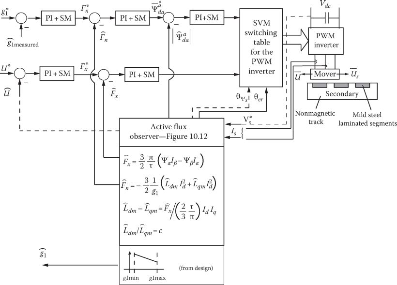
FIGURE 10.14 DTFC of L-RSM for integrated propulsion and suspension control in MAGLEVs.

10.9 Summary

Linear reluctance synchronous motors have a uniformly slotted primary core that hosts a three-phase ac winding and a variable reluctance laminated passive long secondary; the absence of PMs and of a secondary winding is the main merit of L-RSM in terms of costs/performance.
Medium- and high-speed transportation and low-speed short travel industrial propulsion (and controlled magnetic suspension) in MAGLEVs or wheel (or linear bearing) suspension are the main applications of L-RSMs.
The rather large airgap (6 ÷ 10 mm) in medium- to high-speed MAGLEVs leads to a laminated–segmented pole secondary with medium saliency ratio (for costs reason) that provides good efficiency, but at 0.5 ÷ 0.6 power factor, which means high PWM inverter kVA on board of vehicle; as the L-RSM is capable to provide integrated propulsion and levitation control with standard PWM inverter vector DTFC, this drawback may be an acceptable compromise.
For low-speed (1 ÷ 3 m/s) short travel transport applications in industry at an airgap of 0.5 1 mm), good saliency (L_dm/L_qm = 6 ÷ 8) may be obtained with MFB (axially laminated anisotropic equivalent) secondary; thus, a power factor above 0.7 may be obtained for reasonable efficiency (75% ÷ 80%): this compares reasonably even with linear PM synchronous motors of similar thrust and speed, as seen in subsequent chapters.
With 2p ≥ 6 poles, the dynamic (and static) longitudinal effect is negligible, and thus, the theory of rotary RSMs may be applied to L-RSM; for small L-RSMs (with 2p ≥ 2, 4), direct 2(3)D FEM analysis is to be used to precisely assess the performance, as current asymmetry due to static longitudinal end effect is notable.
L-RSM is characterized by an 8 (15) to 1 normal force to thrust ratio, and thus, it is preferable for integrated propulsion and levitation (MAGLEV) applications. To avoid noise and vibration in low-speed applications, the levitation control may produce controlled normal force to cover 90% of mover rated load weight or full levitation control to put to use the large normal force of L-RSM.
The efficiency of L-RSM does not decay notably with load, and the normal force increases slightly with load for constant voltage and constant speed. This property offers plenty of room for adequate propulsion and levitation efficient control.
The design methodology introduced in this chapter for low-speed short travel applications is based on two key conditions at maximum speed:
- Maximum thrust per flux for peak short duration thrust
- Maximum power factor for rated thrust
For a 0.8 kN rated and 1.6 kN peak thrust at 2 m/s application, a 32 kg primary L-RSM was designed; it provides a maximum ideal acceleration of five times the gravity.
A vector control system based on the “active flux” model transplanted from rotary RSMs is introduced for propulsion-only control.
For motion sensorless integrated propulsion and levitation control, a DTFC system (based also on the “active flux” model) is introduced to produce a robust control system.
L-RSM, better in performance than LIM in well-defined conditions, simple, and rugged, with low-cost passive track (secondary) and integrated propulsion–levitation features, without PMs, may not be ruled out in transportation and industrial applications.
In terms of research, core loss, thrust pulsation reduction, optimal design for application, and better integrated propulsion-levitation control are fields that seem worthy of generous talents in the near future.

References

1. P. Lawrenson and S.K. Gupta, Developments in the performance and theory of segmental rotor reluctance motors, Proc. IEEE, 114(5), 1967, 645–653.

2. B.J. Chalmers and A.C. Williams, Ac Machines: Electromagnetics & Design, John Wiley & Sons, New York, 1991, 75–85.

3. A.I.O. Cruickshank and R.W. Menzies, Axially laminated anisotropic rotors for reluctance motors, Proc. IEEE, 113, 1966, 2058–2060.

4. I. Boldea, Reluctance Synchronous Machines and Drives, Clarendon Press, Oxford, U.K., 1996.

5. A. Vagati, G. Franceskini, I. Marongiu, and G.P. Troglia, Design criteria for high performance synchronous reluctance motors, Record of IEEE—IAS-1992, Houston, TX, vol. 1, pp. 66–73.

6. I. Boldea, Z.H. Fu, and S.A. Nasar, Performance evaluation of ALA rotor reluctance synchronous machine, Record of IEEE—IAS-1992, Houston, TX, vol. 1, pp. 212–218.

7. S. Masayuki, S. Morimoto, and Y. Takeda, Thrust ripple improvement of linear synchronous motor with segmented mover construction, Record of LDIA 2001, Nagano, Japan, pp. 451–455.

8. I. Boldea, M.C. Paicu, and G.D. Andreescu, Active flux concept for motion-sensorless unified ac drives, IEEE Trans., PE-23(5), 2008, 2612–2618.

..................Content has been hidden....................

You can't read the all page of ebook, please click here login for view all page.

Table of Contents for Chapter 10 Linear Reluctance Synchronous Motors: Modeling, Performance Design, and Control

Create new playlist

Sign In

Sign Up

Modeling, Performance Design, and Control

Table of Contents for
Chapter 10 Linear Reluctance Synchronous Motors: Modeling, Performance Design, and Control