Chapter 8 Superconducting Magnet Linear Synchronous Motors

Search in book...
Toggle Font Controls
Create new playlist

Name your new playlist

Playlist description (optional)
Sign In

Email address

Password

Forgot Password?

or

Continue with Facebook

Continue with Google
Sign Up

Full Name

Email address

Confirm Email Address

Password

or

Continue with Facebook

Continue with Google

Superconducting magnet linear synchronous motors (SM-LSM) with active guideway have been proposed for MAGLEVs, at speeds up to 550 km/h so far. This chapter treats the following aspects of SM-LSMs:

Topologies of practical interest
Superconducting magnet (SM)
A technical field and circuit theory of SM-LSM
Normal and lateral forces
SM-LSM with figure eight-shape-coil stator
Direct thrust and suspension (airgap) via flux control (DTFC) of SM-LSM
Summary

8.1 Introduction

The SM-LSM consists of dc superconducting coils (magnets) placed on the mover (vehicle) and an active guideway with three-phase air-core cable windings placed horizontally (Figure 8.1) or vertically (laterally on the two sides of the track) (Figure 8.2).

While both configurations (with rectangular and, respectively, figure 8-shape coils) of stator windings develop in interaction with the SM field, propulsion, suspension, and lateral forces, the latter is better in force density and dynamics and was proposed to integrate the three functions in a MAGLEV.

In this chapter, to elucidate the fundamentals, we will treat first the configuration in Figure 8.1 and only later the configuration in Figure 8.2, as the latter is more complicated to analyze.

Other early configurations such as the Magneplane [2] are not considered here as they have not been proved practical though they are very intuitive.

The air-core cable three-phase ac windings on ground (on both sides of the vehicle for MAGLEVs) allow for longer energized sections because the total inductance per section is lower in air. The SM-LSM is preferred for even higher speeds as the airgap is in the order of 5–10 cm or more, while it is 10 mm for dc-excited LSMs (Chapter 7). The larger airgap means rougher guideways, at lower cost. The alternate polarity SMs placed along the vehicle length produce a traveling magnetic field by motion, at speed u_s = u. The pole pitch of SMs and of stator windings is the same (τ), and the frequency f₁ of stator currents speed u_s is

f_{1} = \frac{u_{s}}{2 τ} (8.1)

$f_{1} = \frac{u_{s}}{2 τ} (8.1)$

As for any synchronous motor, to vary speed u_s, the frequency f₁ has to be varied from zero. The key element of SM-LSM is the SM (coil).

Images

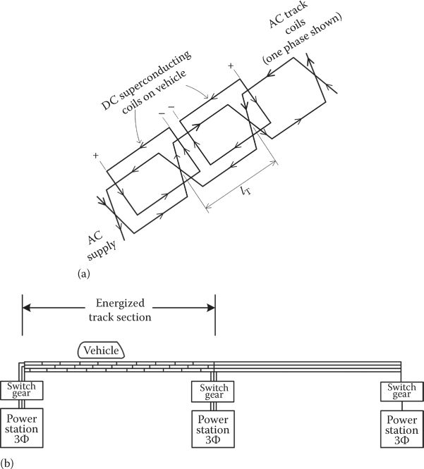
FIGURE 8.1 SM-LSM: (a) SMs on vehicle and air-core three-phase cable windings on ground and (b) three-phase track energized sections. (After Nasar, S.A. and Boldea, I., Linear Motion Electric Machines, John Wiley & Sons, New York, 1976.)

Images

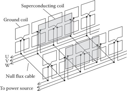
FIGURE 8.2 Figure eight-shape-coil three-phase ac winding with propulsion, suspension, and guidance force production. (After Toshiaki, M. and Shunsuke, F., Design of coil specifications in EDS Maglev using an optimization program, Record of LDIA-1998, Tokyo, Japan, pp. 343–346, 1998.)

8.2 Superconducting Magnet

Kamerlingh Onnes has observed around 1911 that some metals lose most of their electrical resistance below 10 K; the transition from natural to superconducting behavior is called critical temperature T_c (T_c = 9.1 K for niobium); aluminum, indium, tin, lead, niobium, and their alloys are superconductors at very low temperatures. A regular supply of liquid helium and liquid nitrogen on board of vehicle (or a dedicated refrigerator) are required to maintain this range of temperatures (bellow 10 K). More recently, high-temperature (70 K) superconductors that need only liquid nitrogen cooling have been discovered (for more on applied superconductivity, see [3,4]).

A typical SM of low temperature (Figure 8.3) contains

Superconducting coil
Liquid helium dewar
Liquid nitrogen dewar
Evacuated fiberglass insulation

The liquid nitrogen dewar is made of aluminum, and the liquid helium dewar is fabricated from stainless steel (to reduce eddy current losses).

The evacuated fiberglass insulation has very low thermal conductivity, can transmit high pressure, and makes the force-density distribution uniform.

The force components between SM and the three-phase ac conductors in an “air core” are exerted directly on the superconducting coil, at gas pressures of 100 μmHg, maintained by a vacuum pump. The SM coil (currents) leads have to be well cooled by additional tubes and posts in the dewars, to streamline the supply of cooling agents properly stored on board of vehicle.

The design, the charging, and discharging of SM such that to avoid quenching (transition to normal conductor from superconducting mode) is an art in itself, which is not pursued here further (either for low- and high-temperature SMs [3]).

In fact, the SM is a superconducting short-circuited coil that maintains the dc current in it constant (if periodical replenishing with current by a special static converter is done properly (slowly), as required, without quenching the superconductor).

The SM may also be compared with a very strong and large permanent magnet; the latter behaves like an equivalent room temperature superconducting coil, but its energy is stored in a large hysteresis cycle strong magnetic material.

It is argued that for large geometries (0.5–1 m in one direction) the SM may produce more thrust (or suspension, guidance) force per given weight or per one USD than a permanent magnet.

With the advent of high-temperature SMs and of ever stronger PMs (B_r > 1.5 T), the competition becomes stronger than ever.

Images

FIGURE 8.3 Low-temperature SM. (After Nasar, S.A. and Boldea, I., Linear Motion Electric Machines, John Wiley & Sons, New York, 1976.)

8.3 Technical Field and Circuit Theory of SM-LSM

Typical SM-LSMs for MAGLEVs have power in the range of 5 MW or more at speeds of 500–550 km/h with energized sections of 3–5 km in length. The dc mmf of LSM is in the order (3 ÷ 7)10⁵ A turns to produce a magnetic flux density of 0.2–0.45 T that interacts with the stator currents to produce propulsion, suspension, (levitation), and lateral forces for an effective gap of 5–10 cm at least (the superconducting coil to winding center to center distance may be as large as 30 cm).

In essence, we have to start with the magnetic field produced by a rectangular SM in air, and then we add the contribution of neighboring SMs of alternate polarity, to obtain the needed magnetic field distribution in the stator three-phase air-core winding zone.

Further on, we will calculate the emfs in the three-phase ac windings; there are three-phase ac winding inductances and resistances to form a phasor diagram that, for the fundamental, describes the steady-state operation. A third space harmonic, which is typical, may be added to reveal essential thrust pulsations.

After steady-state characteristics are obtained, the thrust, normal force, and lateral force versus power angle are calculated, to illustrate the complex behavior of SM-LSM. This is called here the technical circuit theory of SM-LSM.

8.3.1 Magnetic Field of a Rectangular SM in Air

After approximating the conductors by infinitely thin filaments, the flux density produced in point (P) (Figure 8.4a) by a finite length conductor [1] is obtained via Biot-Savart law (Figure 8.4b):

\bar{B_{1}} = \frac{μ_{0} I_{0}}{4 π} - \int_{- l}^{l} \frac{{\bar{d x}}_{1} \times \bar{d r}}{r^{2}} (8.2)

$\bar{B_{1}} = \frac{μ_{0} I_{0}}{4 π} - \int_{- l}^{l} \frac{{\bar{d x}}_{1} \times \bar{d r}}{r^{2}} (8.2)$

with

r_{1} = \sqrt{{(y + b)}^{2} + z^{2}}; r = \sqrt{{(x - x_{1})}^{2} + r_{1}^{2}} (8.3)

$r_{1} = \sqrt{{(y + b)}^{2} + z^{2}}; r = \sqrt{{(x - x_{1})}^{2} + r_{1}^{2}} (8.3)$

and

d \bar{x_{1}} \times d \bar{r} = \frac{r_{1} d \bar{a_{1}}}{\sqrt{{(x - x_{1})}^{2}} + r_{1}^{2}} (8.4)

$d \bar{x_{1}} \times d \bar{r} = \frac{r_{1} d \bar{a_{1}}}{\sqrt{{(x - x_{1})}^{2}} + r_{1}^{2}} (8.4)$

Images

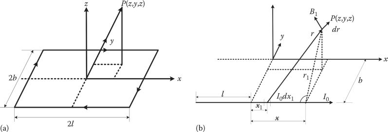
FIGURE 8.4 Rectangular SM (a) and the magnetic field produced by a finite length conductor (b). (After Nasar, S.A. and Boldea, I., Linear Motion Electric Machines, John Wiley & Sons, New York, 1976.)

$\bar{a_{1}}$ $\bar{a_{1}}$ is the unit vector in the direction of the plane formed by point P and the conductor finite length. As visible in Figure 8.4, $\bar{a_{1}}$ $\bar{a_{1}}$ has two components $\bar{a_{y}}$ $\bar{a_{y}}$ and $\bar{a_{z}}$ $\bar{a_{z}}$ :

{\bar{a}}_{1} = \frac{z}{\sqrt{{(y + b)}^{2} + z^{2}}} {\bar{a}}_{y} + \frac{(b + y)}{\sqrt{{(y + b)}^{2} + z^{2}}} {\bar{a}}_{z} (8.5)

${\bar{a}}_{1} = \frac{z}{\sqrt{{(y + b)}^{2} + z^{2}}} {\bar{a}}_{y} + \frac{(b + y)}{\sqrt{{(y + b)}^{2} + z^{2}}} {\bar{a}}_{z} (8.5)$

Finally, from (8.2) to (8.5),

B_{1 y} = \frac{μ_{0} I_{0}}{4 π} \frac{z}{\sqrt{{(y + b)}^{2} + z^{2}}} \int_{- l}^{l} \frac{\sqrt{{(y + b)}^{2} + z^{2}} d x_{1}}{{[{(x - x_{1})}^{2} + {(y + b)}^{2} + z^{2}]}^{3 / 2}} (8.6)

$B_{1 y} = \frac{μ_{0} I_{0}}{4 π} \frac{z}{\sqrt{{(y + b)}^{2} + z^{2}}} \int_{- l}^{l} \frac{\sqrt{{(y + b)}^{2} + z^{2}} d x_{1}}{{[{(x - x_{1})}^{2} + {(y + b)}^{2} + z^{2}]}^{3 / 2}} (8.6)$

B_{1 z} = \frac{μ_{0} I_{0}}{4 π} \frac{b + y}{\sqrt{{(y + b)}^{2} + z^{2}}} \int_{- l}^{l} \frac{\sqrt{{(y + b)}^{2} + z^{2}} d x_{1}}{{[{(x - x_{1})}^{2} + {(y + b)}^{2} + z^{2}]}^{3 / 2}} (8.7)

$B_{1 z} = \frac{μ_{0} I_{0}}{4 π} \frac{b + y}{\sqrt{{(y + b)}^{2} + z^{2}}} \int_{- l}^{l} \frac{\sqrt{{(y + b)}^{2} + z^{2}} d x_{1}}{{[{(x - x_{1})}^{2} + {(y + b)}^{2} + z^{2}]}^{3 / 2}} (8.7)$

A rectangular SM has four sides. Thus, the flux density produced at point P adds up the components produced by the four SM sides and exhibits all three components B_x, B_y, B_z:

\begin{array}{l} B_{x} = \frac{μ_{0} I_{0}}{4 π} z {\frac{1}{{(x - l)}^{2} + z^{2}} [\frac{y + b}{\sqrt{{(x - l)}^{2} + {(y + b)}^{2} + z^{2}}} - \frac{y - b}{\sqrt{{(x - l)}^{2} + {(y - b)}^{2} + z^{2}}}] \\ - \frac{1}{{(x - l)}^{2} + z^{2}} [\frac{y + b}{\sqrt{{(x + l)}^{2} + {(y + b)}^{2} + z^{2}}} \frac{y - b}{\sqrt{{(x + l)}^{2} + {(y - b)}^{2} + z^{2}}}]} \end{array} (8.8)

$\begin{array}{l} B_{x} = \frac{μ_{0} I_{0}}{4 π} z {\frac{1}{{(x - l)}^{2} + z^{2}} [\frac{y + b}{\sqrt{{(x - l)}^{2} + {(y + b)}^{2} + z^{2}}} - \frac{y - b}{\sqrt{{(x - l)}^{2} + {(y - b)}^{2} + z^{2}}}] \\ - \frac{1}{{(x - l)}^{2} + z^{2}} [\frac{y + b}{\sqrt{{(x + l)}^{2} + {(y + b)}^{2} + z^{2}}} \frac{y - b}{\sqrt{{(x + l)}^{2} + {(y - b)}^{2} + z^{2}}}]} \end{array} (8.8)$

\begin{array}{l} B_{y} = \frac{μ_{0} I_{0}}{4 π} z {\frac{1}{{(y - b)}^{2} + z^{2}} [\frac{x + l}{\sqrt{{(x + l)}^{2} + {(y - b)}^{2} + z^{2}}} - \frac{x - l}{\sqrt{{(x - l)}^{2} + {(y - b)}^{2} + z^{2}}}] \\ - \frac{1}{{(y + b)}^{2} + z^{2}} [\frac{x + l}{\sqrt{{(x + l)}^{2} + {(y + b)}^{2} + z^{2}}} \frac{x - l}{\sqrt{{(x - l)}^{2} + {(y + b)}^{2} + z^{2}}}]} \end{array} (8.9)

$\begin{array}{l} B_{y} = \frac{μ_{0} I_{0}}{4 π} z {\frac{1}{{(y - b)}^{2} + z^{2}} [\frac{x + l}{\sqrt{{(x + l)}^{2} + {(y - b)}^{2} + z^{2}}} - \frac{x - l}{\sqrt{{(x - l)}^{2} + {(y - b)}^{2} + z^{2}}}] \\ - \frac{1}{{(y + b)}^{2} + z^{2}} [\frac{x + l}{\sqrt{{(x + l)}^{2} + {(y + b)}^{2} + z^{2}}} \frac{x - l}{\sqrt{{(x - l)}^{2} + {(y + b)}^{2} + z^{2}}}]} \end{array} (8.9)$

\begin{array}{l} B_{z} = \frac{μ_{0} I_{0}}{4 π} z {\frac{(y + b)}{{(y + b)}^{2} + z^{2}} [\frac{x + l}{\sqrt{{(x + l)}^{2} + {(y + b)}^{2} + z^{2}}} - \frac{(x - l)}{\sqrt{{(x - l)}^{2} + {(y + b)}^{2} + z^{2}}}] \\ - \frac{(y - b)}{{(y + l)}^{2} + z^{2}} [\frac{x + l}{\sqrt{{(x + l)}^{2} + {(y - b)}^{2} + z^{2}}} \frac{(x - l)}{\sqrt{{(x - l)}^{2} + {(y - b)}^{2} + z^{2}}}]} \end{array} (8.10)

$\begin{array}{l} B_{z} = \frac{μ_{0} I_{0}}{4 π} z {\frac{(y + b)}{{(y + b)}^{2} + z^{2}} [\frac{x + l}{\sqrt{{(x + l)}^{2} + {(y + b)}^{2} + z^{2}}} - \frac{(x - l)}{\sqrt{{(x - l)}^{2} + {(y + b)}^{2} + z^{2}}}] \\ - \frac{(y - b)}{{(y + l)}^{2} + z^{2}} [\frac{x + l}{\sqrt{{(x + l)}^{2} + {(y - b)}^{2} + z^{2}}} \frac{(x - l)}{\sqrt{{(x - l)}^{2} + {(y - b)}^{2} + z^{2}}}]} \end{array} (8.10)$

Images

FIGURE 8.5 Rectangular SM coil: Normal flux density B_z distribution (a) versus motion direction Ox, (b) versus transverse direction Oy. (After Nasar, S.A. and Boldea, I., Linear Motion Electric Machines, John Wiley & Sons, New York, 1976.)

For a numerical example with the data speed u_s = 130 m/s; f₁ = 50 Hz; 2b = 0.8 m; 2l = 1 m, z = 0.3 m, l_T = 1.3 m (Figure 8.4). I₀ = 3.5 × 10⁵ A turns, the B_z distribution along motion direction x and transverse direction y are shown in Figure 8.5a,b.

There is a notable flux density outside the SM (|x| > l), which means that if the distance between neighboring SMs is about the same as the airgap length (z), the magnetic field sensed by the armature winding at a point comprises contributions of a few (say three) SMs.

8.3.2 EMF E₁ Inductance and Resistance L_s, R_s per Phase

The flux variation in a stator coil, placed at distance x with respect to the SM center, is thus

\frac{d Φ}{d x} = \int_{- b}^{b} B_{z} (x, y, z) d y (8.11)

$\frac{d Φ}{d x} = \int_{- b}^{b} B_{z} (x, y, z) d y (8.11)$

The voltage induced in a track coil by a single SM, E_SM, is

E_{S M} = u_{s} \frac{d Φ}{d x} (8.12)

$E_{S M} = u_{s} \frac{d Φ}{d x} (8.12)$

For three-SM contribution, the total emf in a stator coil E₀ is

E_{0} = u_{s} \sum_{n = 1}^{3} \frac{d Φ}{d x} (8.13)

$E_{0} = u_{s} \sum_{n = 1}^{3} \frac{d Φ}{d x} (8.13)$

If the vehicle has N SMs per side, the emf in the stator phase E₁ is

E_{1} = N E_{0} (8.14)

$E_{1} = N E_{0} (8.14)$

The shape of dΦ/dx is essential for current shape control. For sinusoidal (vector) current control, the emf has to be almost sinusoidal, in order to produce low thrust pulsations.

For τ = 1 m and SM length/pole pitch L/τ = 0.7, z₀ = 0.2 m (airgap), I₀ = 5 × 10⁵ A turns, 2b = 0.9 m, dΦ/dx is close to a sinusoidal (Figure 8.6); not so for τ = 4 m. Investigating for optimal pole pitch and L/τ and “stack” width/pole pitch ratio, 2b/τ, is a must if the emf shape is to be the desired one (sinusoidal in general).

The armature (stator) mmf produced magnetic field is notably smaller than that of the SMs. Consequently, the armature inductance per phase, L_ph, for an energized section of 2p′ poles may be calculated as for long electric power lines:

L_{p h} \approx \frac{μ_{0}}{π} {4 p^{'} l \times \ln [\frac{τ}{d} + {[{(\frac{τ}{d})}^{2} - 1]}^{1 / 2}] + 2 p^{'} τln {[\frac{l}{d} + [{(\frac{l}{d})}^{2} - 1]]}^{1 / 2}} (8.15)

$L_{p h} \approx \frac{μ_{0}}{π} {4 p^{'} l \times \ln [\frac{τ}{d} + {[{(\frac{τ}{d})}^{2} - 1]}^{1 / 2}] + 2 p^{'} τln {[\frac{l}{d} + [{(\frac{l}{d})}^{2} - 1]]}^{1 / 2}} (8.15)$

where

d is the diameter of armature coil conductor

l is the armature coil width

The resultant inductance L_s per phase, including the influence of the other two phases, is

L_{s} \approx L_{p h} (1 + \frac{1}{3} + \frac{1}{6}) (8.16)

$L_{s} \approx L_{p h} (1 + \frac{1}{3} + \frac{1}{6}) (8.16)$

The armature resistance/phase R_s writes

R_{s} \approx \frac{ρ_{A l}}{2 q_{A l}} (l + τ) 2 p^{'} \times K_{l} K_{s k i n} (8.17)

$R_{s} \approx \frac{ρ_{A l}}{2 q_{A l}} (l + τ) 2 p^{'} \times K_{l} K_{s k i n} (8.17)$

where

ρ_Al is the aluminum electric resistivity

q_Al is the aluminum cable cross section

K_l = 1.05–1.2 accounts for the departure of stator coils from rectangular shape

K_skin > 1 accounts for skin effect in the stator conductors

The factor 2 accounts for the situation when two cables in parallel make the phase winding (Figure 8.1).

Note on skin effect: As the stator current with cable winding is rather large, in the 2000 A or more range, for a more than 5 MW propulsion vehicle, the skin effect should be reduced and, anyway, considered in the cable design (multiple-conductor twisted cable is to be used).

Images

FIGURE 8.6 Rate of SM flux change with position. (After Boldea, I. and Nasar, S.A., Linear Motion Electromagnetic Systems, Wiley & Sons, New York, 1985.)

8.3.3 Phasor Diagram, Power Factor, and Efficiency

The phasor diagram is valid only for sinusoidal emf; a practical waveform is shown in Figure 8.7; it contains some third and fifth time harmonics, which may be generating thrust pulsations if the third harmonic occurs in current (delta connections of phases).

Such delta connection of phases is feasible as it allows connection of an energized section from both ends (Figure 8.8).

Images

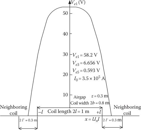
FIGURE 8.7 Emf in a track coil. (After Nasar, S.A. and Boldea, I., Linear Motion Electric Machines, John Wiley & Sons, New York, 1976.)

Images

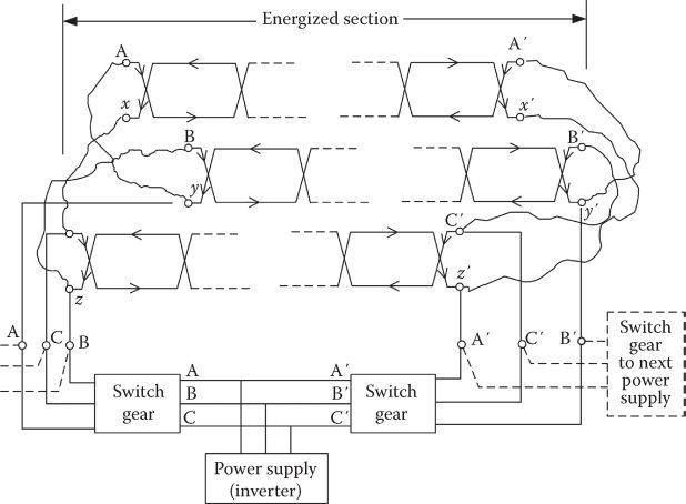
FIGURE 8.8 Delta connection of stator-phase sections. (After Nasar, S.A. and Boldea, I., Linear Motion Electric Machines, John Wiley & Sons, New York, 1976.)

For the fundamental, the voltage equation per phase is

\begin{array}{l} \underline{V_{1}} = R_{s} \underline{I_{1}} + j ω_{1} L_{s} \underline{I_{1}} - E_{1} e^{- j δ_{v}}; & ω_{1} \end{array} = \frac{π u_{s}}{τ}, (8.18)

$\begin{array}{l} \underline{V_{1}} = R_{s} \underline{I_{1}} + j ω_{1} L_{s} \underline{I_{1}} - E_{1} e^{- j δ_{v}}; & ω_{1} \end{array} = \frac{π u_{s}}{τ}, (8.18)$

where

V₁ is the applied phase voltage fundamental

I₁ is the phase current fundamental

δ_v is the power angle (Figure 8.9)

Images

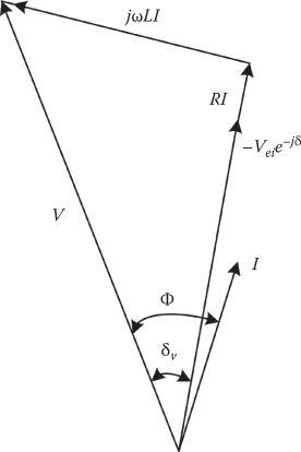
FIGURE 8.9 Phasor diagram. (After Nasar, S.A. and Boldea, I., Linear Motion Electric Machines, John Wiley & Sons, New York, 1976.)

The phase current I₁ is simply

\underline{I_{1}} = \frac{1}{Z_{1}^{2}} {[(V_{1} - E_{1} \cos δ_{v}) R_{s} + ω_{1} L_{s} E_{1} \sin δ_{v}] - j [ω_{1} L_{s} (V_{1} - E_{1} \cos δ_{v}) - R_{s} E_{1} \sin δ_{v}]} (8.19)

$\underline{I_{1}} = \frac{1}{Z_{1}^{2}} {[(V_{1} - E_{1} \cos δ_{v}) R_{s} + ω_{1} L_{s} E_{1} \sin δ_{v}] - j [ω_{1} L_{s} (V_{1} - E_{1} \cos δ_{v}) - R_{s} E_{1} \sin δ_{v}]} (8.19)$

\cos φ_{1} = \frac{1}{{1 + {[\frac{ω_{1} L_{s} (V_{1} - E_{1} \cos δ_{v}) - R_{s} E_{1} \sin δ_{v}}{(V_{1} - E_{1} \cos δ_{v}) R_{s} + ω_{1} L_{s} E_{1} \sin δ_{v}}]}^{2}}^{1 / 2}} (8.20)

$\cos φ_{1} = \frac{1}{{1 + {[\frac{ω_{1} L_{s} (V_{1} - E_{1} \cos δ_{v}) - R_{s} E_{1} \sin δ_{v}}{(V_{1} - E_{1} \cos δ_{v}) R_{s} + ω_{1} L_{s} E_{1} \sin δ_{v}}]}^{2}}^{1 / 2}} (8.20)$

with

Z = R_{s} + j ω_{1} L_{s} (8.21)

$Z = R_{s} + j ω_{1} L_{s} (8.21)$

Finally, the active and reactive powers are obtained from

| S | = | P - j Q | = 3 V_{1} I_{1} (8.22)

$| S | = | P - j Q | = 3 V_{1} I_{1} (8.22)$

\frac{1}{Z_{s}^{2}} [V_{1} R_{s} (V_{1} - E_{1} \cos δ_{v}) + ω_{1} L_{s} V_{1} E_{1} \sin δ_{v}] (8.23)

$\frac{1}{Z_{s}^{2}} [V_{1} R_{s} (V_{1} - E_{1} \cos δ_{v}) + ω_{1} L_{s} V_{1} E_{1} \sin δ_{v}] (8.23)$

In a dc-excited LSM, the power factor could be adjusted by controlling the dc field current. This is not the case with SM-LSM, where equivalent dc mmf in SM is rather constant.

The thrust F_x₁ is

F_{x 1} = \frac{P_{1} - 3 R_{s} | I_{1}^{2} |}{U_{s}} = \frac{3 E_{1} | I_{1} | \cos (δ_{v} - ϕ)}{U_{s}} (8.24)

$F_{x 1} = \frac{P_{1} - 3 R_{s} | I_{1}^{2} |}{U_{s}} = \frac{3 E_{1} | I_{1} | \cos (δ_{v} - ϕ)}{U_{s}} (8.24)$

For a Δ connection of phases, the third harmonic current $\underline{I_{3}}$ $\underline{I_{3}}$ in the stator, due to emf third harmonic emf, is obtained from the equation

R_{s 3} \underline{I_{3}} + j 3 ω_{1} L_{s} \underline{I_{3}} - E_{3} e^{- j 3 δ_{v}} = 0 (8.25)

$R_{s 3} \underline{I_{3}} + j 3 ω_{1} L_{s} \underline{I_{3}} - E_{3} e^{- j 3 δ_{v}} = 0 (8.25)$

The apparent third harmonic power $\underline{S_{3}}$ $\underline{S_{3}}$ is

\underline{S_{3}} = P_{3} - j Q_{3} = \frac{{| E_{3} |}^{2}}{R_{s 3} + j 3 ω_{1} L_{s}} (8.26)

$\underline{S_{3}} = P_{3} - j Q_{3} = \frac{{| E_{3} |}^{2}}{R_{s 3} + j 3 ω_{1} L_{s}} (8.26)$

Skin effect is more important at 3ω₁, and thus, we have introduced R_S₃ instead of R_s.

In a three-phase circuit, the third harmonic currents are in phase, and thus, the instantaneous power pulsates at frequency 6ω₁, leading to additional losses $(3 r_{s_{2}} {| \underline{I_{3}} |}^{2})$ $(3 r_{s_{2}} {| \underline{I_{3}} |}^{2})$ and to thrust F_x₃:

F_{x 3} = \frac{3 P_{3}}{U_{s}} (1 - \cos 6 ω_{1} t) (8.27)

$F_{x 3} = \frac{3 P_{3}}{U_{s}} (1 - \cos 6 ω_{1} t) (8.27)$

The total thrust F_x is

F_{x} = F_{x_{1}} + F_{x_{3}} (8.28)

$F_{x} = F_{x_{1}} + F_{x_{3}} (8.28)$

The efficiency is thus

η \approx \frac{F_{x a v} U_{s}}{3 V_{1} I_{1} \cos φ_{1}} (8.29)

$η \approx \frac{F_{x a v} U_{s}}{3 V_{1} I_{1} \cos φ_{1}} (8.29)$

8.3.4 Numerical Example 8.1

Let us illustrate the SM-LSM performance, as extracted from the so far developed technical theory, versus voltage power angle δ_v, for the following initial specifications:

Input voltage V₁ = 4200 V (peak phase value), f₁ = 50 Hz, SM mmf I₀ = 3.5 × 10⁵ A turns, u_s = 130 m/s, SM dimensions 2l = 1 m, 2b = 0.8 m, number of SMs = 32, energized track length = 2 km, delta connection R_s = 0.18 Ω, L_s = 4.22 mH, and airgap z = 0.3 m.

From Figure 8.7 (which uses the same data), we may calculate E₁, E₃(E₅, I₅ are neglected):

\begin{array}{l} E_{1} = 32 \times 58.21 \sqrt{2} = 1316 V \\ E_{3} = 32 \times 6.65 \sqrt{2} = 150 V \end{array} (8.30)

$\begin{array}{l} E_{1} = 32 \times 58.21 \sqrt{2} = 1316 V \\ E_{3} = 32 \times 6.65 \sqrt{2} = 150 V \end{array} (8.30)$

Images

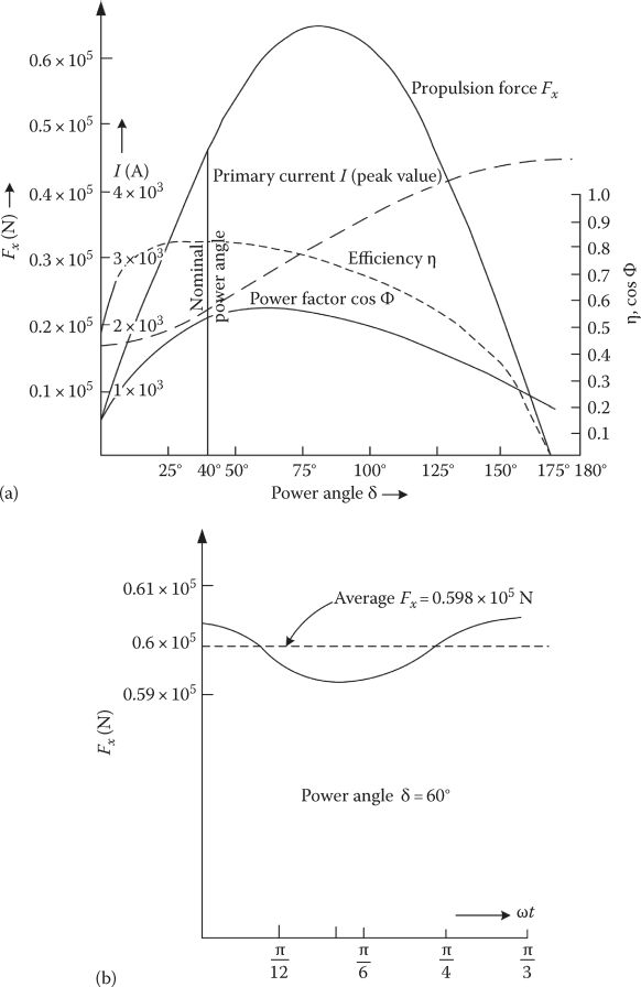
FIGURE 8.10 SM-LSM performance (a) and thrust pulsations (b). (After Nasar, S.A. and Boldea, I., Linear Motion Electric Machines, John Wiley & Sons, New York, 1976.)

From (8.19) to (8.29), the results in Figure 8.10 are obtained.

For the rated power angle δ_v = 40°, F_xav = 0.469 × 10⁵ N, η_n = 0.82, cos φ₁ = 0.53, and I_n = 2241 A (peak value).

The thrust pulsations with δ_v = 60° are shown in Figure 8.10b.

8.4 Normal and Lateral Forces

As already stated, besides propulsion force (thrust) the SM-LSM develops also normal and lateral force. The normal force F_z acts perpendicularly to the motion direction and, in our case (of horizontal stator), it is vertical; F_z may be an attraction or a repulsive force, which is nonzero for symmetric or asymmetric placement of stator and SMs (Figure 8.11a).

Images

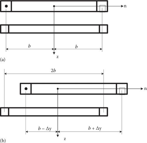
FIGURE 8.11 Symmetric (a) and asymmetric placement of SMs and track coils (b). (After Nasar, S.A. and Boldea, I., Linear Motion Electric Machines, John Wiley & Sons, New York, 1976.)

The lateral force F_y occurs only in case of laterally asymmetric placement of stator and SMs (Figure 8.11b); this asymmetry may be produced by wind or other perturbation forces.

In general an attraction (unstable) normal force is accompanied by a restoring (stabilizing) lateral force, and a repulsion-type normal force coexists with a decentralizing lateral force, to fulfill the Earnshaw’s theorem.

It would be ideal to stabilize by the converter control both propulsion and suspension, from zero (or small) speed upward and, eventually, stabilize separately the guidance (produced by lateral forces). The figure eight-shape-coil vertical SM-LSM attempts just that. But, to reveal the modeling of normal and lateral forces, we keep the simple rectangular coil stator winding placed asymmetrically (Figure 8.11b). For one phase of the three-phase stator, the normal and lateral forces (F_z, F_y) (with N SMs on vehicle) are [6]

\begin{array}{l} {(F_{z})}_{p h a s e} = N I_{0} i_{a} \frac{\partial M_{s t}}{\partial z} \\ {(F_{y})}_{p h a s e} = N I_{0} i_{a} \frac{\partial M_{s t}}{\partial y} \end{array} (8.31)

$\begin{array}{l} {(F_{z})}_{p h a s e} = N I_{0} i_{a} \frac{\partial M_{s t}}{\partial z} \\ {(F_{y})}_{p h a s e} = N I_{0} i_{a} \frac{\partial M_{s t}}{\partial y} \end{array} (8.31)$

where

I = SM mmf

i_a is the phase current

M_st is the mutual inductance between the SM and phase a track coil

The total forces add up the contributions of all three stator phases.

As the instantaneous phase currents i_a, i_b, i_c may be calculated from (8.19) for given V₁, speed (frequency), and power angle δ_v, only the mutual inductances M_st. (i = a, b, c) have to be calculated.

A generic SM and one-phase track coil placed asymmetrically are shown in Figure 8.12.

Images

FIGURE 8.12 SM and stator coil, and asymmetric SM/stator placement. (After Nasar, S.A. and Boldea, I., Linear Motion Electric Machines, John Wiley & Sons, New York, 1976.)

The SM and track coil lengths are different from each other $({i^{'}}_{T} \neq {i^{'}}_{t})$ $({i^{'}}_{T} \neq {i^{'}}_{t})$ , but the pole pitch is the same, and the lateral asymmetry is portrayed by b₁(b + Δy) ≠ b₂(b – Δy). The Neumann inductance formula writes

M_{s t 0} = \frac{μ_{0}}{4 π} \int_{c_{1}} \int_{c_{2}} \frac{d x d x^{'} + d y d y^{'} + d z d z^{'}}{{[{(x - x^{'})}^{2} + {(y - y^{'})}^{2} + {(z - z^{'})}^{2}]}^{1 / 2}} (8.32)

$M_{s t 0} = \frac{μ_{0}}{4 π} \int_{c_{1}} \int_{c_{2}} \frac{d x d x^{'} + d y d y^{'} + d z d z^{'}}{{[{(x - x^{'})}^{2} + {(y - y^{'})}^{2} + {(z - z^{'})}^{2}]}^{1 / 2}} (8.32)$

where xyz and x′y′z′ are coordinates of one point on the stator coil and, respectively, on SM, with c₁, c₂ as the contours of the two coils. The contours c₁ and c₂ are defined by A′, B′,C′,D′ $({x^{'}}_{o i}, {y^{'}}_{o i}, {z^{'}}_{o i}, i = 1, 2, 3, 4)$ $({x^{'}}_{o i}, {y^{'}}_{o i}, {z^{'}}_{o i}, i = 1, 2, 3, 4)$ and by A, B, C, D (x_oj, y_oj, z_oj, j = 1, 2, 3, 4).

The integral in (8.32) leads to

M_{s t 0} = \frac{μ_{0}}{4 π} \sum_{j = 1}^{4} \sum_{j = 1}^{4} {(- 1)}^{i + j} [ψ (x_{0 j}, y_{o j}, 0; {x^{'}}_{0 i}, {y^{'}}_{0 i}, z_{0}) + ψ (y_{o j}, x_{0 j}, 0; {y^{'}}_{0 i}, {x^{'}}_{0 i} z_{0})] (8.33)

$M_{s t 0} = \frac{μ_{0}}{4 π} \sum_{j = 1}^{4} \sum_{j = 1}^{4} {(- 1)}^{i + j} [ψ (x_{0 j}, y_{o j}, 0; {x^{'}}_{0 i}, {y^{'}}_{0 i}, z_{0}) + ψ (y_{o j}, x_{0 j}, 0; {y^{'}}_{0 i}, {x^{'}}_{0 i} z_{0})] (8.33)$

with

ψ (x, y, z, x^{'}, y^{'}, z^{'}) = - (x - x^{'}) \ln [(x - x^{'}) + \sqrt{{(x - x^{'})}^{2} + {(y - y^{'})}^{2} + {(z - z^{'})}^{2}}] (8.34)

$ψ (x, y, z, x^{'}, y^{'}, z^{'}) = - (x - x^{'}) \ln [(x - x^{'}) + \sqrt{{(x - x^{'})}^{2} + {(y - y^{'})}^{2} + {(z - z^{'})}^{2}}] (8.34)$

There are many (n) stator coils of alternate polarity that interact with one SM, and thus, the total mutual inductance adds up all these components:

\begin{array}{l} M_{s t} = {(- 1)}^{n + 1} \frac{μ_{0}}{4 π} \sum_{n = 0}^{\infty} \sum_{j = 1}^{4} \sum_{j = 1}^{4} {(- 1)}^{i + j} [ψ (x_{n j}, y_{n j}, 0; {x^{'}}_{0 i}, {y^{'}}_{0 i}, z_{0}) + ψ (y_{n j}, x_{n j}, 0; {y^{'}}_{0 i}, {x^{'}}_{0 i} z_{0})] \\ + {(- 1)}^{n} \frac{μ_{0}}{4 π} \sum_{n = 0}^{\infty} \sum_{j = 1}^{4} \sum_{j = 1}^{4} {(- 1)}^{i + j} [ψ (x_{- n j}, y_{- n j}, 0; {x^{'}}_{0 i}, {y^{'}}_{0 i}, z_{0}) + ψ (y_{- n j}, x_{- n j}, 0; {y^{'}}_{0 i}, {x^{'}}_{0 i} z_{0})] \end{array} (8.35)

$\begin{array}{l} M_{s t} = {(- 1)}^{n + 1} \frac{μ_{0}}{4 π} \sum_{n = 0}^{\infty} \sum_{j = 1}^{4} \sum_{j = 1}^{4} {(- 1)}^{i + j} [ψ (x_{n j}, y_{n j}, 0; {x^{'}}_{0 i}, {y^{'}}_{0 i}, z_{0}) + ψ (y_{n j}, x_{n j}, 0; {y^{'}}_{0 i}, {x^{'}}_{0 i} z_{0})] \\ + {(- 1)}^{n} \frac{μ_{0}}{4 π} \sum_{n = 0}^{\infty} \sum_{j = 1}^{4} \sum_{j = 1}^{4} {(- 1)}^{i + j} [ψ (x_{- n j}, y_{- n j}, 0; {x^{'}}_{0 i}, {y^{'}}_{0 i}, z_{0}) + ψ (y_{- n j}, x_{- n j}, 0; {y^{'}}_{0 i}, {x^{'}}_{0 i} z_{0})] \end{array} (8.35)$

Both left- and right-side stator coils around each SM have been considered in (8.35).

The coordinates in (8.35)—Figure 8.12—are

\begin{array}{l} {x^{'}}_{01} = {x^{'}}_{04} = u_{s} t + x_{m} + \frac{1}{2} {l^{'}}_{T} \\ {x^{'}}_{02} = {x^{'}}_{03} = u_{s} t + x_{m} - \frac{1}{2} {l^{'}}_{T} \\ {y^{'}}_{01} = {y^{'}}_{02} = b + Δ y \\ {y^{'}}_{03} = {y^{'}}_{04} = - b + Δ y \\ x_{n 1} = x_{n 4} = \frac{1}{2} {l^{'}}_{t} + (n - 1) l_{t} \\ x_{n 2} = x_{n 3} = \frac{1}{2} {l^{'}}_{t} + (n - 1) l_{t} \\ x_{- n 1} = - x_{- n 4} = \frac{1}{2} {l^{'}}_{t} - n l_{t} \\ x_{- n 2} = - x_{- n 3} = - \frac{1}{2} {l^{'}}_{t} - n l \\ y_{n 1} = y_{n 2} = b = y_{- n 1} = y_{- n 2} \\ y_{n 3} = y_{n 4} = - b = y_{- n 3} = y_{- n 4} \end{array} (8.36)

$\begin{array}{l} {x^{'}}_{01} = {x^{'}}_{04} = u_{s} t + x_{m} + \frac{1}{2} {l^{'}}_{T} \\ {x^{'}}_{02} = {x^{'}}_{03} = u_{s} t + x_{m} - \frac{1}{2} {l^{'}}_{T} \\ {y^{'}}_{01} = {y^{'}}_{02} = b + Δ y \\ {y^{'}}_{03} = {y^{'}}_{04} = - b + Δ y \\ x_{n 1} = x_{n 4} = \frac{1}{2} {l^{'}}_{t} + (n - 1) l_{t} \\ x_{n 2} = x_{n 3} = \frac{1}{2} {l^{'}}_{t} + (n - 1) l_{t} \\ x_{- n 1} = - x_{- n 4} = \frac{1}{2} {l^{'}}_{t} - n l_{t} \\ x_{- n 2} = - x_{- n 3} = - \frac{1}{2} {l^{'}}_{t} - n l \\ y_{n 1} = y_{n 2} = b = y_{- n 1} = y_{- n 2} \\ y_{n 3} = y_{n 4} = - b = y_{- n 3} = y_{- n 4} \end{array} (8.36)$

where x_m is the position of the center of SM at t (time) = 0. As expected, M_st is a periodic function with respect to position x (or time):

M_{s t} = \sum_{k = 1}^{\infty} M_{s t k} \cos \frac{k}{l_{t}} (π u_{s} t + π x_{m}) (8.37)

$M_{s t} = \sum_{k = 1}^{\infty} M_{s t k} \cos \frac{k}{l_{t}} (π u_{s} t + π x_{m}) (8.37)$

The position x_m is related to the power angle δ_v (Figure 8.9):

\begin{matrix} \frac{π x_{m}}{l_{t}} = \frac{π}{2} - δ_{v}; & ω_{1} = \frac{π u_{s}}{l_{t}} \end{matrix} (8.38)

$\begin{matrix} \frac{π x_{m}}{l_{t}} = \frac{π}{2} - δ_{v}; & ω_{1} = \frac{π u_{s}}{l_{t}} \end{matrix} (8.38)$

M_st may be written as

M_{s t} = \sum_{k = 1}^{\infty} M_{s t k} \cos k (ω_{1} t + \frac{π}{2} - δ_{v}) (8.39)

$M_{s t} = \sum_{k = 1}^{\infty} M_{s t k} \cos k (ω_{1} t + \frac{π}{2} - δ_{v}) (8.39)$

Let us now suppose that the phase stator current has two components:

i_{a} = i_{1} + i_{3} = I \sqrt{2} \cos (ω_{1} t - φ) - I_{3} \sqrt{2} \cos (3 ω_{1} t - δ_{v} - φ_{3}) (8.40)

$i_{a} = i_{1} + i_{3} = I \sqrt{2} \cos (ω_{1} t - φ) - I_{3} \sqrt{2} \cos (3 ω_{1} t - δ_{v} - φ_{3}) (8.40)$

with

φ_{3} = \tan^{- 1} (3 ω_{1} L_{S} / R_{S}) . (8.41)

$φ_{3} = \tan^{- 1} (3 ω_{1} L_{S} / R_{S}) . (8.41)$

From (8.31) to (8.41) and considering all three phases, the normal and lateral forces F_z and F_y are

F_{z, y} = 3 N I_{0} {\begin{matrix} I \frac{\partial (M_{s t 1})}{\partial z, y} \sin (δ_{v} - φ_{1}) - I_{3} \frac{\partial (M_{s t 3})}{\partial z, y} [\sin φ_{3} - \sin (6 ω_{1} t - 6 δ_{v} - φ_{3})] \\ + I \frac{\partial (M_{s t 5})}{\partial z, y} \sin (6 ω_{1} t - 5 δ_{v} - φ_{1}) \end{matrix}} (8.42)

$F_{z, y} = 3 N I_{0} {\begin{matrix} I \frac{\partial (M_{s t 1})}{\partial z, y} \sin (δ_{v} - φ_{1}) - I_{3} \frac{\partial (M_{s t 3})}{\partial z, y} [\sin φ_{3} - \sin (6 ω_{1} t - 6 δ_{v} - φ_{3})] \\ + I \frac{\partial (M_{s t 5})}{\partial z, y} \sin (6 ω_{1} t - 5 δ_{v} - φ_{1}) \end{matrix}} (8.42)$

where N is the number of SMs per vehicle.

8.4.1 Numerical Example 8.2

For the same data as in Example 8.1, and no lateral asymmetry, applying the earlier formulae, the normal force F_n is calculated and shown in Figure 8.13a,b.

From Figure 8.13a, it is evident that the normal force changes from attraction to repulsion mode. The lateral force is zero as Δy = 0 (symmetric SM stator location).

Next, we consider a lateral displacement Δy = 3.5 cm. Only the lateral force is shown in Figure 8.14a,b.

At δ_v = 55°, again, the lateral force switches from restoring to decentralizing mode.

Discussion

Propulsion force is produced at reasonable efficiency and power factor for δ_v = 40° − 100°; for vector control, the power angle may be controlled as needed.
Unfortunately, in its rectangular stator-coil configuration, the normal and lateral forces are not very large for δ_v = 40° − 100°, but they both pass through zero at δ_v = 55°.
As the inverter on ground may control only the current amplitude I₁ and the power angle δ_v, it follows that only two forces may be controlled at any time.
Also, the propulsion and normal forces are of the same order of magnitudes, and thus, the latter is very far from the level needed for full suspension of the vehicle through SM-LSM. For 1 m/s² acceleration, the normal force has to be 10 times larger than the propulsion force, to fully suspend magnetically the vehicle.
These remarks suggest that for fully integrated propulsion, suspension, and some guidance, the eight-shape-stator-coil lateral stators on ground configuration are required.

8.5 SM-LSM with Eight-Shape-Stator Coils

The eight-shape-stator-coil configuration (Figure 8.1) was conceived to produce thrust and normal and guidance (lateral) forces in a controlled manner to be sufficient for a MAGLEV. This is a departure from the standard system, which has special short-circuited coils on track for suspension and guidance.

Images

FIGURE 8.13 Average normal force, (a) and normal force pulsations at δ_v = 60° (b). (After Nasar, S.A. and Boldea, I., Linear Motion Electric Machines, John Wiley & Sons, New York, 1976.)

Figure 8.15a adds the generator coils onboard the vehicle, placed between the SMs and the stator coils, and the eight-shape-stator coils. SM-LSM main geometry parameters are given in Figure 8.15b.

The linear generator “collects” the power through electromagnetic induction from the stator mmf space harmonics (especially the 5th harmonic). The generator tooth-wound coils pole pitch τ₂ = (4/15)τ; τ-main pole pitch.

The eight-shape-stator coils (Figure 8.3) are connected in series, and they are concentrated coils (with q = 0.5): three of them side by side make a pole pitch (Figure 8.15c), 3τ₁ = τ. This leads to a lower winding factor (0.867), but it is easy to build and install.

There are also connections of eight-shape-stator coils of the two sides of the vehicle (Figure 8.3) to create opposite lateral forces to “centralize” the vehicle, for damping of the eventual oscillations. These connections are called null-flux cables on Figure 8.2.

To elevate the stability between vehicle guidance and rolling motion, the eight-shape figure is made asymmetric, with the lower part taller than the upper part (Figure 8.15a), though this merit is accompanied by an increase in the take-off velocity [7].

The reverse current direction in the upper and lower parts of eight-shape coils enhances levitation (propulsion) force, while the reverse current between left- and right-side coils increases the lateral force. The circulating currents induced by SMs through motion are producing the bulk of levitation and lateral forces.

Images

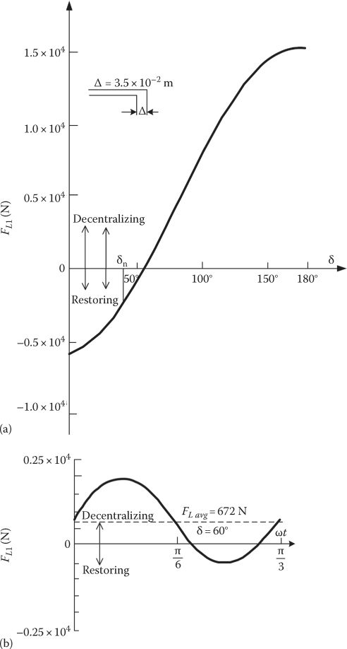
FIGURE 8.14 Average lateral force (Δy = 3.5 cm) (a) and its pulsations at δ_v = 60° (b). (After Nasar, S.A. and Boldea, I., Linear Motion Electric Machines, John Wiley & Sons, New York, 1976.)

A design optimization attempt should observe quite a few constraints such as

Levitation (vertical) force F_z (in this case) balances the required force (vehicle weight) at both take-off (u₁) and cruising (u₂) speed, when the thrust levels are different from each other.
Equivalent guidance and rolling stiffness, $F_{y y}^{*}$ $F_{y y}^{*}$ and $M_{ϕ ϕ}^{*}$ $M_{ϕ ϕ}^{*}$ , should exceed the requirements at take-off speed u₁, where they are minimum by nature.
Propulsion force F_x balances the total drag force load F_xload at cruising speed u₂, where, in general, propulsion requirements are maximum (acceleration force during starting is not larger).
Linear generator power P_g exceeds the requirements above a certain speed (it could be cruising speed u₂, but, better, a smaller value).

Images

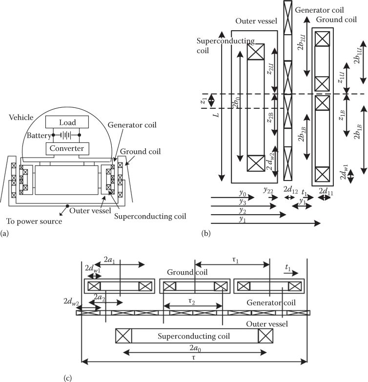
FIGURE 8.15 Integrated propulsion-levitation guidance system. (a) coil composition, (b) transverse cross section, (c) cross and longitudinal geometries. (After Toshiaki, M. and Shunsuke, F., Design of coil specifications in EDS Maglev using an optimization program, Record of LDIA-1998, Tokyo, Japan, pp. 343–346, 1998.)

Besides constraints such as earlier, quite a few objective functions (or combination of them) can be put into place:

Minimization of magnetic drag F_mdrag produced by the eight-shape-stator-coil circulating currents by which most levitation (suspension) is produced, at take-off and (or) at cruising speed u₂).
Maximization of guidance stiffness $F_{y y}^{*}$ $F_{y y}^{*}$ at take-off speed u₁.
Optimization of propulsion performance in terms of efficiency or power factor.
Maximization of linear generator output power P₂ at cruising speed.
For given take-off speed u₁ and linear generator power P₂, the required propulsion power P₁ (which accounts for accelerating power plus covering the magnetic drag F_mdrag and air drag F_adrag of vehicle) may be minimized [8].

It goes without saying that using each objective function leads the optimization routine (quasi-Newton method with Karush–Kuhn–Tucker conditions) to a different design.

With four poles and two rows of SMs, on a bogie we treat (Tables 8.1 and 8.2), in fact, only eight SMs’ performance.

TABLE 8.1
Specification of MAGLEV Systems and Coils

Images

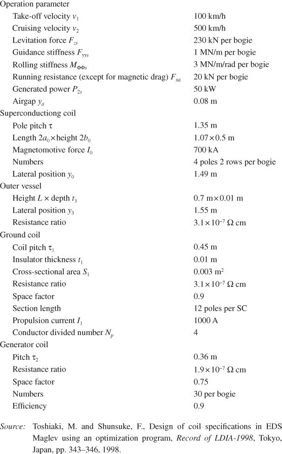
TABLE 8.2
Maximized Specifications for Each System

Images

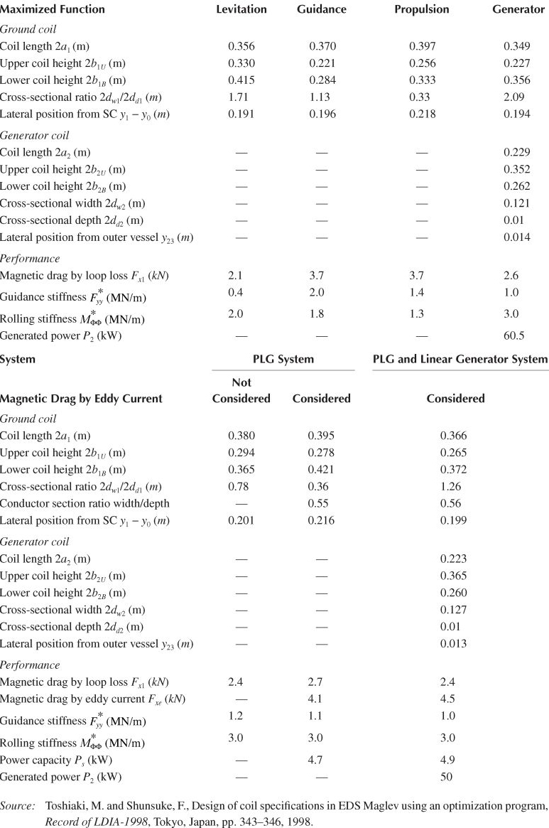
Table 8.1 [7] shows typical specifications for one 230 kN bogie, 500 km/h SM-LSM MAGLEV. Table 8.2 shows typical objective function specification design results [7].

Table 8.2 shows clearly that four different designs are obtained based on the four main objective functions, and thus, a global cost function has to be added to discriminate between them. Combining 1–2 objective functions would lead to yet other designs.

8.6 Control of SM-LSM

Combined propulsion and levitation control has to be attempted from start (especially for eight-shape-coil stators). Both flux-oriented control (FOC) and direct thrust and flux control (DTFC) may be adopted for this air-core machine with constant dc mmf excitation but variable average airgap z (Figure 8.16).

Images

FIGURE 8.16 Generic DTFC of superconducting LSM (a) with state observer (b).

Today’s power electronics is better prepared for FOC or DTFC, even for powers of 5–10 MW, at 6 kV and f ≈ U_max/2τ = 130/(2 · 1) = 65 Hz. Even pole pitches τ smaller than 1 m are feasible for a lateral distance of 0.2–0.3 m between SMs and stator (the mechanical gap is 5–10 cm).

Note: We should mention again that the bulk of the repulsion-type (statically stable) levitation and guidance is produced by the circulating currents induced by the SMs (by motion) in the stator eight-shape coils at “the cost” of a magnetic drag force F_mdrag. These aspects will be treated in a later chapter dedicated to magnetic suspension systems.

A generic DTFC for SM-LSM is shown in Figure 8.16, where the thrust is controlled directly for propulsion and the SM flux channel is used to dynamically control levitation. This means implicit control of stator currents I₁ and power angle δ_v.

DTFC does not need SM position feedback for control directly, other than for the flux observer at low speeds; the speed u is anyway measured and used to compensate emf and provide for cruising control.

A peculiarity of SM-LSM is that the stator inductance L_s and resistance are rather constant (rather independent of airgap z): the temperature influence on R_s may be needed during vehicle starting, for more robust control.

A special control method for starting may be needed for a motion-sensorless control.

The compensator voltage V_comp in Figure 8.16b may be based on a current model of the machine:

V_{c o m p} = P_{i} [{\bar{Ψ}}_{s} - {\bar{Ψ}}_{s i}] (8.43)

$V_{c o m p} = P_{i} [{\bar{Ψ}}_{s} - {\bar{Ψ}}_{s i}] (8.43)$

The current model based observer ${\bar{Ψ}}_{s i}$ ${\bar{Ψ}}_{s i}$ used back and forth in stator to mover to stator coordinates is shown in Figure 8.17. Both ${\hat{θ}}_{m o v e r}$ ${\hat{θ}}_{m o v e r}$ and $\bar{Z}$ $\bar{Z}$ estimation are obtained, as needed for motion-sensorless control.

Safety precautions impose multiple airgap sensors on board vehicle in key points; their output has to be transmitted wirelessly to the ground station for control. Especially for protection, as all controls are provided on ground, the DTFC system is basically sensorless and it works as such but, in practice, it may be used merely for redundancy.

Quenching of SMs (eight in all on a bogie in our case study) would severely disturb the vehicle stable ride, and thus, a symmetrically placed additional SM is quenched intentionally [9]. But the faulty bogie has still to be capable to handle the entire weight for suspension although at a smaller (but not dangerous) airgap z_min. The SMs experience induced eddy current losses due to both the ac fields of stator mmf and of linear generator mmf [10]. Other specific phenomena pertaining to SM-LSM such as active track inverter supply section by section in a synchronized manner will be dealt with in a later chapter dedicated to active guideway MAGLEVs.

Images

FIGURE 8.17 Flux ${\overset{⌢}{Ψ}}_{s}^{s}$ ${\overset{⌢}{Ψ}}_{s}^{s}$ and airgap $\overset{⌢}{Z}$ $\overset{⌢}{Z}$ observer.

8.7 Summary

SMs are air-core coils enclosed in dewars to keep them at low temperatures (10 K or less respectively 77 K or less) such that the conductor resistivity drops 10⁵ times with respect to normal temperatures; so once the SM is charged with a dc current the latter stays there for hours and days and may be slowly refilled, such that to avoid notable eddy current losses that may quench (turn from superconductor to normal conductor mode) the SM [11].
It is argued that for large flat coil sizes the SM is economically feasible and is even better than the large permanent magnet (for same weight or cost), in terms of electromagnetic propulsion, levitation, and guidance at very high speeds and large effective gaps between vehicle and guideway (5–10 cm).
A row of alternate polarity SMs on the vehicle behaves like a constant field current excitation (or PM) for the air-core stator three-phase winding placed along the track (travel) length and ac fed through inverters on ground in sections of a few kilometers.
Horizontal placement of SMs below the floor of the vehicle with flat rectangular three-phase cable windings with stator (active track) is natural, and this configuration was first used to investigate thoroughly the SM-LSM modeling and performance via a technical field and circuit theory.
The technical theory starts with the calculation of the magnetic flux-density components B_x, B_y, B_z in a point in air by an air-core rectangular SM of given dc mmf I₀ (Ampere turns); fortunately there is an analytical approach that saves time, when a computer code is used.
For adequate combinations of airgap z, pole pitch of SM spreading τ(l_T) per coil length and coil width/pole pitch, the emf E₁, produced by motion by the SM in a track (stator) coil, shows close to a sinusoidal waveform in time for given vehicle speed.
The active section air-core stator windings cyclic inductance per phase (L_s) is rather independent of SM-LSM airgap and is calculated as for long power transmission lines; the active section (phase) resistance R_s expression is also straightforward.
With E₁, R_s, L_s of SM-LSM, steady-state (or transient) equations, as a nonsalient-pole synchronous machine, are straightforward; the accompanying phasor diagram serves to calculate the phase current ${\underline{I}}_{1}$ ${\underline{I}}_{1}$ (amplitude and phase angle) for given speed u, stator phase voltage V₁, and power angle δ_v.
Through a numerical example with $V_{1} = 4200 / \sqrt{2}$ $V_{1} = 4200 / \sqrt{2}$ RMS value phase, u = 130 m/s, I₀ = 3, 5 × 10⁵ A turns, 2l = 1 m, 2b = 0.8 m, 32 SMs per vehicle, z = 0.3 m (theoretical airgap), f₁ = 50 at δ_v = 40°, F_xav = 0, 47 × 10⁵ N, η = 0.82, cos φ₁ = 0.53, which could be considered acceptably good performance.
To investigate normal force F_z, and lateral force F_y of an SM-LSM, the vehicle is placed laterally asymmetric.
Based on Neumann inductance formula applied for the double row of SMs and respectively, stator coils, all three forces F_x, F_y, F_z are calculated for given stator-phase current, speed, and power angle δ_v.
It is shown that in our case study, the normal force is of attraction character for δ_v < 55° and repulsive for δ_v > 55°.
The lateral force is nonzero only when lateral asymmetry (Δy) is present; it also changes from restoring force below δ_v = 55° (in our case study) to decentralizing force for δ_v > 55°.
However, the normal and lateral forces are of the order of magnitude of propulsion force for the rectangular stator-coil SM-LSM investigated so far; so they are far away from the high values (10 times higher) needed for full suspension. Separate short-circuited coils along the guideway may be placed to produce full levitation of the vehicle. Alternatively, the eight-shape-stator-coil (null-flux) winding is used to produce all three forces in sufficient amplitudes and fully controlled.
The eight-shape-stator coils of stator interact three ways with the SMs row in vehicle:
- The motion-induced circulating currents in the eight-shape coils interact with the SMs and produce a levitation force F_n (besides a magnetic drag force F_mdrag).
- The same motion-induced circulating currents, which also circulate laterally from left- to right-side coils produce the lateral force F_y that restores the lateral motion equilibrium.
- Finally, the ac stator currents interact with the SM row field to produce three forces F_x, F_y, F_z; the first one F_x propulses the vehicle; the other two F_y, F_z related to one another and of similar magnitude serve to control (damp) various vehicle oscillatory parasitic motions.
- Magnetic levitation performance will be discussed in a dedicated later chapter.
The SM-LSM control system may control only the thrust and, say, the stator flux to control suspension/levitation via average airgap z control.
A generic DTFC system is introduced and detailed in the situation of any motion-sensor absence; an actual vehicle has quite a few airgap sensors (at least for safety), and thus, sensorless control may be used only for redundancy.
Design optimization methods [7] for eight-shape-stator-coil SM-LSM have been proven capable to lead to good performance, and the full-scale vehicle at Yamanashi track in Japan seems to validate them satisfactorily.
Very similar in behavior to SM-LSM, the air-core PM active guideway LSM has been proposed for urban MAGLEVs first in Germany and then recently in USA; so the air-core SM-LSM or PM-LSM with active guideway is open for new developments.

References

1. S.A. Nasar and I. Boldea, Linear Motion Electric Machines, Chapter 5, John Wiley & Sons, New York, 1976.

2. M.M. Kolm, R.D. Thornton, Y. Kwasa, and W.S. Brown, The magneplane system, Cryogenics, 15(7), July 1975, 377–383.

3. I. Sakamoto, Vertical electromagnetic force of a superconducting LSM vehicle based on the formulation in dq axes, Record of LDIA-2001, Nagano, Japan, pp. 149–153.

4. J.R. Schreiffer and J.S. Brooks (eds.), Handbook of High Temperature Superconductivity: Theory end Experiment, Springer Verlag, New York, 2007.

5. I. Boldea and S.A. Nasar, Linear Motion Electromagnetic Systems, Chapter 5, Wiley & Sons, New York, 1985.

6. E. Ohno, M. Iwamoto, and T. Yamada, Characteristics of superconductive suspension and propulsion for high speed trains, Proc. IEEE, 61(5), 1973, pp. 579–586.

7. M. Toshiaki and F. Shunsuke, Design of coil specifications in EDS Maglev using an optimization program, Record of LDIA-1998, Tokyo, Japan, pp. 343–346.

8. T. Murai and S. Fujiwara Characteristics of combined propulsion levitation and guidance system with asymmetric figure between upper and lower coils in EDS, Record of LDIA-1995, Nagasaki, Japan, pp. 37–46.

9. O. Shunsuke, O. Hiroyuki, and E. Masada, Stabilizing the motion of the superconducting magnetically levitated train against coil quenching, Record of LDIA-1998, Tokyo, Japan, pp. 339–342.

10. H. Hasegawa, T. Murai, and T. Sasakawa, Electromagnetic analysis of eddy current loss in superconducting magnet for MAGLEV, Record of LDIA-2001, Nagano, Japan, pp. 315–322.

11. F.C. Moon, Superconducting Imitation, John Wiley & Sons, New York, 1997.

..................Content has been hidden....................

You can't read the all page of ebook, please click here login for view all page.

Table of Contents for Chapter 8 Superconducting Magnet Linear Synchronous Motors

Create new playlist

Sign In

Sign Up

Table of Contents for
Chapter 8 Superconducting Magnet Linear Synchronous Motors