Chapter 11 Linear Switched Reluctance Motors (L-SRM): Modeling, Design, and Control

Search in book...
Toggle Font Controls
Create new playlist

Name your new playlist

Playlist description (optional)
Sign In

Email address

Password

Forgot Password?

or

Continue with Facebook

Continue with Google
Sign Up

Full Name

Email address

Confirm Email Address

Password

or

Continue with Facebook

Continue with Google

Modeling, Design, and Control

Linear switched reluctance motors (L-SRMs) are counterparts of rotary switched reluctance motors [1–3]. The finite length of their magnetic circuit along the direction of motion introduces, for a small number of poles, some longitudinal static effects (asymmetries between phases). Also, the normal force has its peculiarities with L-RSM, but other than that, the theory developed for rotary SRMs may be adapted easily for linear SRMs.

So, as for rotary SRMs, L-SRM produces a thrust and motion by the tendency of a ferromagnetic secondary to hold a position where inductance of the active (excited) primary phase is maximum. Though it is in general a multiphase machine, L-SRM operates with 1(2) phases as active at any time. The turning on and off of each phase is triggered by a linear position sensor or by an observer so as to fully exploit the thrust capability of that phase. So the turning on and off of each phase is “in tact” (synchronous) with rotor position; however, each phase is fully energized and deenergized for each thrust cycle, and thus L-SRMs are not traveling field synchronous machines (like L-RSMs in the previous chapter). This brings L-SRM closer to linear stepper motors, but with position control of each phase current. Finally, the mutual inductances between phases in L-SRMs are small, which is good for fault tolerance but it is the reason why all the energization and deenergization cycling process takes place through the special PWM inverter (multiphase dc–dc converter) that supplies it.

The rather low thrust density of L-SRM (unless very heavily saturated) in comparison with linear PM synchronous motors) is another secondary effect of its simplicity and low cost. The L-SRM’s ruggedness and rather low losses recommend it for linear motion application in various industries.

11.1 Practical Topologies

L-SRMs have a longitudinal or transverse lamination uniformly slotted primary core with tooth-wound (concentrated) 1, 2, 3, 4, or more phase coils and a variable reluctance longitudinal or a transverse-lamination secondary core. The pole pitches τ_s, τ_p of the slottings of the primary and secondary are in general

τ_p=τ_s (N_s=N_r) one-phase cores for single-phase L-SRMs with “stepped” airgap for self-starting (Figure 11.1)
τ_p/τ_s=4/6 or 8/6 (N_s=6, N_r=4, 8 or multiples of these values) for three phases (Figure 11.2)
τ_p/τ_s=6/8 (N_s = 8, N_r=6, 10 etc.) for four phases (Figure 11.3)

The principle is that each secondary pole is attracted to the active phase poles when the latter is supplied with a PWM voltage to produce a mover-position-triggered phase unipolar current in that phase.

While single-sided, flat, three-phase configurations with longitudinal and transverse flux are shown in Figure 11.2, a double-sided flat four-phase configuration is shown in Figures 11.3. In Figures 11.1 through 11.3, the mover is active (primary), and thus it must be supplied by a flexible ac power cable in short travel applications or by a mechanical (or inductive) power transfer on board in transportation (or special clean room) applications.

Images

FIGURE 11.1 Single-phase, saturated, half-secondary pole, flat, single-sided L-RSM and its thrust versus position for constant current fixed secondary.

Images

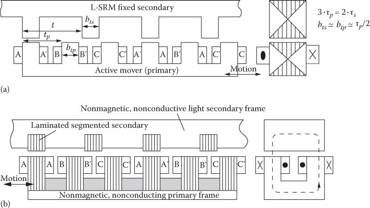
FIGURE 11.2 Three-phase, flat, single-sided L-SRM: (a) longitudinal and (b) transverse.

Images

FIGURE 11.3 Four-phase, double-sided, flat L-RSM with active mover (primary) and longitudinal flux.

Tubular configurations may also be adopted for short travel taking advantage of the “blessing” of circularity (Figure 11.4). The tubular L-SRM cores may be made of soft magnetic composites (tooth by tooth in the primary) or from two types of disk-shaped laminations with radial slits, to reduce eddy current losses in the back cores (in not so high fundamental frequency (below 100 Hz) applications).

The ratio between normal force and thrust in L-RSM is rather large (F_n/F_x > 10), and thus, unless F_n is required for levitation, it is just a source of noise, vibration, and, consequently of stress in the iron cores and in the frame. Double-sided flat and tubular topologies implicitly provide zero-ideal normal force on the interior part of L-SRM [2-5].

Images

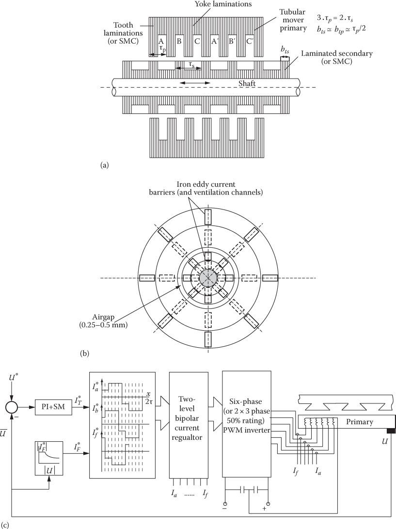
FIGURE 11.4 Three-phase tubular L-RSM with disk-shaped laminations, (a) radial slits (as barriers for eddy currents) (b), and generic control system (c).

The transverse-flux TF-L-SRM is characterized by shorter flux lines and possibly lower core losses, while the iron core usage is poorer, especially in three-phase L-RSMs, where only one phase is active at any time. While typical L-SRMs use tooth-wound coils to reduce copper losses drastically, segmented or multiple flux-barrier secondaries may also be used with multiphase diametrical windings and bipolar two-level current control, for example (Figure 11.5).

This machine has a single magnetic saliency (in the secondary), but it is controlled by bipolar two-level current pulses triggered “in tact” with the mover position. In general, the two phases with the coils around axis q (of lower inductance) play the role of “excitation” coils, and the ones below the secondary poles play the role of thrust coils. This machine, in fact (here in its linear configuration), rather directly mimics the dc brush machine with separate excitation but in its brushless version. Therefore, this would be a “true” brushless dc linear machine without PMs. One phase commutates all the time but the rest are active, and thus a rather high thrust density is provided, with reasonable peak kVA rating in the multiphase inverter.

The field current control level I∗p $I_{p}^{*}$ may be performed to control the airgap and thus provides controlled magnetic levitation in a MAGLEV with good overall performance.

Images

FIGURE 11.5 Six-phase, bipolar, two-level current L-SRM (a), its phase current waveform (b) An ALA secondary generic control system (c)

Images

11.2 Principle of Operation

Let us consider an elementary single-phase L-SRM (Figure 11.6).

To assess the thrust correctly, the energy conservation principle has to be applied:

d W e = d W m e c + d W m; d W m e c = F x d x electric mechanical stored input output magnetic energy energy energy (11.1)

$\begin{array}{l} d W_{e} = d W_{m e c} + d W_{m}; d W_{m e c} = F_{x} d x \\ electric mechanical stored \\ input output magnetic \\ energy energy energy \end{array} (11.1)$

As demonstrated in Chapter 1 the thrust is

F x = - (\partial W m \partial x) ψ = c o n s t .; W m = \int 0 ψ i \cdot d ψ (11.2)

$F_{x} = - {(\frac{\partial W_{m}}{\partial x})}_{ψ= c o n s t .}; W_{m} = \int_{0}^{ψ} i \cdot d ψ (11.2)$

Images

FIGURE 11.6 Elementary single-phase L-SRM.

F x = (\partial W ' m \partial x) i = c o n s t .; W' m = \int 0 i ψ \cdot d i; W m + W' m = i \cdot ψ (11.3)

$F_{x} = {(\frac{\partial W_{m}^{'}}{\partial x})}_{i = c o n s t .}; W_{m}^{'} = \int_{0}^{i} ψ \cdot d i; W_{m} + W_{m}^{'} = i \cdot ψ (11.3)$

Only for a nonsaturated core (ψ(i) are straight lines)

L = L (x) (11.4)

$L = L (x) (11.4)$

W m = W' m = L ( x ) \cdot i 2 2 (11.5)

$W_{m} = W_{m}^{'} = \frac{L (x) \cdot i^{2}}{2} (11.5)$

And thus the thrust F_x and the normal attraction force F_n are

F x i = i 2 2 \partial L \partial x; F n i = i 2 2 \partial L \partial g (11.6)

$F_{x i} = \frac{i^{2}}{2} \frac{\partial L}{\partial x}; F_{n i} = \frac{i^{2}}{2} \frac{\partial L}{\partial g} (11.6)$

For a simplified case, when all fringing flux lines (at the airgap) are neglected and the iron cores permeability is infinite, the inductance L in Figure 11.6 may be written as

L = L l e a k a g e + μ 0 W 21 a \cdot x 2 g; 0 \leq x \leq b p = b s (11.7)

$L = L_{l e a k a g e} + μ_{0} W_{1}^{2} \frac{a \cdot x}{2 g}; 0 \leq x \leq b_{p} = b_{s} (11.7)$

L = L l e a k a g e + μ 0 W 21 a \cdot ( 2 b p - x ) 2 g; b p \leq x \leq 2 b p (11.8)

$L = L_{l e a k a g e} + μ_{0} W_{1}^{2} \frac{a \cdot (2 b_{p} - x)}{2 g}; b_{p} \leq x \leq 2 b_{p} (11.8)$

In this case,

F x i \approx μ 0 W 2 1 i 2 2 \cdot a 2 g = constant > 0 for 0 \leq x \leq b p = b s F n i \approx - μ 0 W 2 1 i 2 2 \cdot a \cdot x 2 g 2 < 0 (11.9)

$\begin{array}{l} F_{x i} \approx \frac{μ_{0} W_{1}^{2} i^{2}}{2} \cdot \frac{a}{2 g} = constant > 0 for 0 \leq x \leq b_{p} = b_{s} \\ F_{n i} \approx - \frac{μ_{0} W_{1}^{2} i^{2}}{2} \cdot \frac{a \cdot x}{2 g^{2}} < 0 \end{array} (11.9)$

and

F x = - μ 0 W 2 1 i 2 2 . a 2 g = constant < 0 for b p \leq x \leq 2 b p F n = μ 0 W 2 1 i 2 a ( 2 b p - x ) g 2 < 0 (11.10)

$\begin{array}{l} F_{x} = - \frac{μ_{0} W_{1}^{2} i^{2}}{2} . \frac{a}{2 g} = constant < 0 for b_{p} \leq x \leq 2 b_{p} \\ F_{n} = \frac{μ_{0} W_{1}^{2} i^{2} a (2 b_{p} - x)}{g^{2}} < 0 \end{array} (11.10)$

As in general g<b_p/4 (to reduce fringing flux) F_y ≫ F_x. The thrust switches from positive to negative values for positive to negative inductance slopes variation with position. The current polarity is irrelevant for thrust and normal force and thus, in general, the L-SRM is supplied from a multiphase dc–dc converter.

Example 11.1

Let us consider an elementary single-phase L-SRM with the data: airgap g = 0.3 m, U-shape core leg width a = 10 mm, the primary and secondary pole length b_p = b_s = 10 mm. Calculate

Thrust and maximum normal force for µ_iron = ∞, Ni=500 A turns
The normal airgap flux density B_g₁
Copper losses for j_Co = 3 A/mm² and coil equal width and height (w_c = h_c)

Solution

1. We may use directly Equation 11.9 for x=b_p:

F x = 1.1256 \times 10 - 6 \times 500 2 2 \times 10 - 2 2 \times 0.3 \times 10 - 3 = 2.616 N (11.11)

$F_{x} = \frac{1.1256 \times 10^{- 6} \times 500^{2}}{2} \times \frac{10^{- 2}}{2 \times 0.3 \times 10^{- 3}} = 2.616 N (11.11)$

F n max = - 1.1256 \times 10 - 6 \times 500 2 \times 10 - 2 \times 10 - 2 4 \times 0.3 2 \times 10 - 6 = - 87.22 N (11.12)

$F_{n \max} = - \frac{1.1256 \times 10^{- 6} \times 500^{2} \times 10^{- 2} \times 10^{- 2}}{4 \times {0.3}^{2} \times 10^{- 6}} = - 87.22 N (11.12)$

With a total active area of primary A = 2a • b_p = 2 cm², it means a specific thrust f_x = 1.308 N/cm² and a specific maximum normal thrust f_n_max = -43.61 N/cm².

2. The normal airgap flux density B_n is

B n = μ 0 W I 2 g = 1.256 \times 10 - 6 \times 500 2 \times 0.3 \times 10 - 3 = 1.0466 T (11.13)

$B_{n} = \frac{μ_{0} W I}{2 g} = \frac{1.256 \times 10^{- 6} \times 500}{2 \times 0.3 \times 10^{- 3}} = 1.0466 T (11.13)$

3. There are two semicoils. The cross section of each of them, A_Co, is

A C o = ( W I 2 ) j C o k f i l l = 500 2 3 \times 0.50 166.66 mm 2 (11.14)

$A_{C o} = \frac{(\frac{W I}{2})}{j_{C o} k_{f i l l}} = \frac{\frac{500}{2}}{3 \times 0.50} 166.66 {mm}^{2} (11.14)$

But ACo=hc⋅wc=h2c=166.66 m m2 $A_{C o} = h_{c} \cdot w_{c} = h_{c}^{2} = 166 . 66 m m^{2}$ , h_c = w_c = 12.91 mm.

The turn average length l_c is

I c \approx 2 a + 2 b p + 4 W c = 2 \times 10 - 2 + 2 \times 10 - 2 + 4 \times 1.291 \times 10 - 2 = 9.164 \times 10 - 2 m (11.15)

$I_{c} \approx 2 a + 2 b_{p} + 4 W_{c} = 2 \times 10^{- 2} + 2 \times 10^{- 2} + 4 \times 1.291 \times 10^{- 2} = 9.164 \times 10^{- 2} m (11.15)$

So the copper losses are

p C o = 2 δ C o I c W j c o i 2 i = 2 δ C o I c W j C o i = 2.21 \times 10 - 8 \times 9.164 \times 10 - 2 \times 250 \times 3 \times 106 = 2.886 W (11.16)

$p_{C o} = \frac{2 δ_{C o} I_{c} W j_{c o} i^{2}}{i} = 2 δ_{C o} I_{c} W j_{C o} i = 2.21 \times 10^{- 8} \times 9.164 \times 10^{- 2} \times 250 \times 3 \times 10^{6} = 2.886 W (11.16)$

Note: Though the numerical example is elementary, the force densities f_x, f_n, and the thrust/losses (N/W) are typical for well-designed practical L-SRMs.

11.3 Instantaneous Thrust

The thrust in (11.9) and (11.10) is constant with mover position but, in reality, due to magnetic saturation variation and due to airgap fringing flux, it is far away from constancy and varies notably with position x and current as seen in what follows. To yield instantaneous thrust, the flux linkage/current/position curves have to be calculated, either analytically (with a multiple magnetic circuit model) or by 2(3) D-FEM; alternatively, it may be measured at standstill from current-decay tests with the primary to secondary position fixed in numerous different situations.

Images

FIGURE 11.7 Standstill test setup to yield flux/current/position curve family decay in aligned and unaligned position: (a) electrical circuit, current decay for aligned, (b) unaligned, and (c) positions.

The dc-dc converter typical for the test is shown in Figure 11.7.

By PWM a certain initial dc current i₀ is installed, and then the switch S is turned off and the current and freewheeling diode voltage decay versus time are recorded. The initial flux linkage in the phase ψ₀, corresponding to initial current i₀, for given mover position x, is obtained by

ψ 0 (i 0, x) = L (i 0, x) \cdot i 0 = \int i . R S \cdot d t + \int V d i o d e \cdot d t (11.17)

$ψ_{0} (i_{0}, x) = L (i_{0}, x) \cdot i_{0} = \int i . R_{S} \cdot d t + \int V_{d i o d e} \cdot d t (11.17)$

The time integrals may be done numerically down to 1%–2% of initial current, to avoid notable errors. Results as in Figure 11.8 are obtained for the family of ψ(i, x) curves. In practice, this family of curves is to be curve-fitted and then used to calculate the thrust, as seen in Figure 11.8:

F x = \partial W ' m \partial x = (Δ W ' m Δ x) i = c o n s t .; Δ x = x A - x B (11.18)

$F_{x} = \frac{\partial W_{m}^{'}}{\partial x} = {(\frac{Δ W_{m}^{'}}{Δ x})}_{i = c o n s t .}; Δ x = x_{A} - x_{B} (11.18)$

Images

FIGURE 11.8 Flux linkage/current/position curves (a) and thrust (F_x) and normal force F_n per phase versus current and position (typical results) (b).

In addition, the normal force may be calculated if the test results are obtained at two close-to-each-other airgaps:

F n = \partial W ' m \partial g = ( Δ W ' m ) Δ g Δ g; W' m = \int 0 i ψ \cdot d i (11.19)

$F_{n} = \frac{\partial W_{m}^{'}}{\partial g} = \frac{{(Δ W_{m}^{'})}_{Δ g}}{Δ g}; W_{m}^{'} = \int_{0}^{i} ψ \cdot d i (11.19)$

The thrust nonuniformity with position is due to both magnetic saturation and fringing airgap flux that vary with mover position. In real operation, the current is flat-top controlled at low speeds and is the result of one voltage pulse per cycle at high speeds (Figure 11.9).

Images

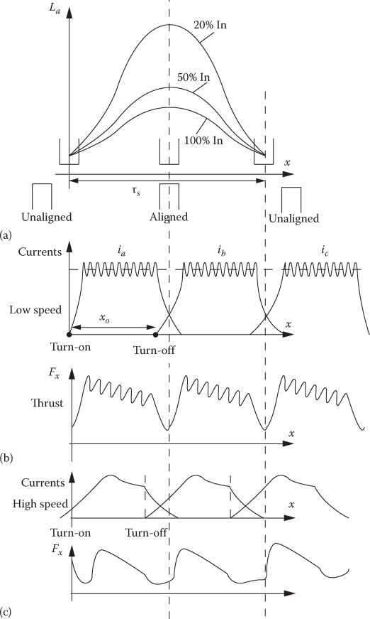
FIGURE 11.9 Three-phase L-SRM: (a) phase inductance (with saturation), (b) flat-top currents and thrust at low speeds, and (c) single voltage pulse current and thrust at high speeds. (After Boldea, I., Variable Speed Generators, CRC Press, Taylor & Francis, Boca Raton, FL, 2006.)

A few remarks are as follows:

The lack of enough voltage at high speeds leads to one pulse voltage/phase/cycle, and anticipated turn on and turn off angles (position) are adopted for higher thrust.
The thrust pulsations inevitably increase with speed and, for three-phase L-SRM, large thrust pulsations remain and thus four-phase L-SRMs with two active phases at any time are needed for low (servo drive class) thrust pulsations (10% or less).

11.4 Average Thrust and Energy Conversion Ratio

(F x) a v p h a s e = W m e c l s t r o k e; l s t r o k e = τ s 2 (11.20)

${(F_{x})}_{p h a s e}^{a v} = \frac{W_{m e c}}{l_{s t r o k e}}; l_{s t r o k e} = \frac{τ_{s}}{2} (11.20)$

For m phases

F x a v = m . N r \cdot W m e c l s t r o k e (11.21)

$F_{x a v} = m . N_{r} \cdot \frac{W_{m e c}}{l_{s t r o k e}} (11.21)$

N_r is the number of secondary poles per primary length.

As some magnetic energy (W_mag in Figure 11.10) is returned to the dc link of the PWM converter, the energy conversion ratio η_ec of the energy cycle is

η e c = W m e c W m e c + W m a g \geq 0.5 (11.22)

$η_{e c} = \frac{W_{m e c}}{W_{m e c} + W_{m a g}} \geq 0.5 (11.22)$

The value of 0.5 is obtained for a linear flux/current variation with flux versus position for all situations; that is, in the absence of magnetic saturation (implicitly at a larger airgap). The energy conversion ratio is a correspondent of the η cos φ product in ac winding, which, in general, is larger than 0.5. So the peak kVA of the PWM inverter for the same speed and thrust is larger for L-SRM. The presence of magnetic saturation increases η_ec to 0.65 ÷ 0.67 while it also decreases the commutation inductance L_t=dψ_t/di allowing for operation at higher speeds. However, magnetic saturation reduces average thrust and leads to larger thrust pulsations for given machine geometry.

Images

FIGURE 11.10 Energy cycle and average thrust/phase.

11.5 CONVERTER RATING

As already stated, the PWM converter has to handle the entire energy per cycle of all phases: m · (W_mec + W_mag). To calculate the converter kVA rating, we start with the flux linkage per phase ψ_C:

ψ C \approx V d c t C = V d c U (x O H - x n) (11.23)

$ψ_{C} \approx V_{d c} t_{C} = \frac{V_{d c}}{U} (x_{O H} - x_{n}) (11.23)$

U is the L-SRM speed.

In terms of energy,

W m e c + W m a g = W m e c η e c = k \cdot ψ C \cdot I C (11.24)

$W_{m e c} + W_{m a g} = \frac{W_{m e c}}{η_{e c}} = k \cdot ψ_{C} \cdot I_{C} (11.24)$

where

I_C is the peak current per phase

k is the so-called converter utilization factor [1]

So the peak kVA S_peak of the m phase L-SRM is (from (11.21) to (11.24))

S p e a k = m V 0 I C = F x m U k \cdot η e c \cdot l s t r o k e x O H - x n = P e l m k \cdot η e c . l s t r o k e x O H - x n (11.25)

$S_{p e a k} = m V_{0} I_{C} = \frac{F_{x m} U}{k \cdot η_{e c}} \cdot \frac{l_{s t r o k e}}{x_{O H} - x_{n}} = \frac{P_{e l m}}{k \cdot η_{e c}} . \frac{l_{s t r o k e}}{x_{O H} - x_{n}} (11.25)$

For η_ec ≤ 0.65, k ≈ 0.7–0.8, l_stroke/(x_OH − x_n) = 1.25, S_peak/P_elm = 2.747. Such values are larger than for typical L-PMSMs (to be treated in a future chapter); it is the price to pay for L-SRM simplicity, fault tolerance, and smaller initial cost.

11.6 State Space Equations and Equivalent Circuit

Let us neglect the mutual flux between L-SRM phases as it is small (less than 3%–4% in general). It means that each phase may be treated separately. The voltage equation for one phase is thus

V = R S I + d ψ ( x , i ) d t; ψ = L (x, i) \cdot i (11.26)

$V = R_{S} I + \frac{d ψ (x, i)}{d t}; ψ = L (x, i) \cdot i (11.26)$

Using the derivative of the flux linkage as product of inductance and current, we obtain first

V = R S I + L t d i d t + \partial L \partial t + \partial L \partial x \cdot i . d x d t; L t = L (x, i) + i \cdot \partial L ( x , i ) \partial i (11.27)

$V = R_{S} I + L_{t} \frac{d i}{d t} + \frac{\partial L}{\partial t} + \frac{\partial L}{\partial x} \cdot \frac{i . d x}{d t}; L_{t} = L (x, i) + \frac{i \cdot \partial L (x, i)}{\partial i} (11.27)$

L_t(x, i) is the so-called transient (or commutation) inductance, which, under magnetic saturation, is even lower than the saturated L(x, i). The third term in (11.27) is speed dependent and may be called the pseudo emf:

E p = \partial L \partial x \cdot i \cdot U; U = d x d t (11.28)

$E_{p} = \frac{\partial L}{\partial x} \cdot i \cdot U; U = \frac{d x}{d t} (11.28)$

Multiplying by i, Equation 11.27 may be written as

v \cdot i = R S I 2 + d d t (1 2 L (x, i) i 2) + 1 2 i 2 d L ( x , i ) d x U (11.29)

$v \cdot i = R_{S} I^{2} + \frac{d}{d t} (\frac{1}{2} L (x, i) i^{2}) + \frac{1}{2} i^{2} \frac{d L (x, i)}{d x} U (11.29)$

The second term coincides with stored magnetic variation in time only when magnetic saturation is constant (∂L/∂i = 0); consequently, only in this case the last term is the mechanical power from which thrust F_x varies:

(F x) \partial L / \partial i = 0 = 1 2 i 2 d L ( x ) d x (11.30)

${(F_{x})}_{\partial L / \partial i = 0} = \frac{1}{2} i^{2} \frac{d L (x)}{d x} (11.30)$

When magnetic saturation is considered, Equations 11.2 and 11.3 for thrust are to be used. For the normal force, Equations 11.29 and 11.30 are to be considered. But in this case, typical when both propulsion and levitation control are performed, the voltage equations (11.27) and (11.28) may be extended as

V = R S I + d ψ ( x , i ) d t + E p + E S; E S = i \partial L ( x , i , g ) \partial g \cdot d g d t (11.31)

$V = R_{S} I + \frac{d ψ (x, i)}{d t} + E_{p} + E_{S}; E_{S} = i \frac{\partial L (x, i, g)}{\partial g} \cdot \frac{d g}{d t} (11.31)$

And again,

E p = i \partial L ( x , i , g ) \partial x \cdot U (11.32)

$E_{p} = i \frac{\partial L (x, i, g)}{\partial x} \cdot U (11.32)$

Similarly, the instantaneous power/phase equation gains an additional term due to vertical (levitation) motion speed:

v \cdot i = R S I 2 + d d t (1 2 L (x, i) i 2) + 1 2 i 2 \partial L ( x , i , g ) \partial x U + 1 2 i 2 \partial L ( x , i , g ) \partial g \cdot d g d t (11.33)

$v \cdot i = R_{S} I^{2} + \frac{d}{d t} (\frac{1}{2} L (x, i) i^{2}) + \frac{1}{2} i^{2} \frac{\partial L (x, i, g)}{\partial x} U + \frac{1}{2} i^{2} \frac{\partial L (x, i, g)}{\partial g} \cdot \frac{d g}{d t} (11.33)$

Based on (11.32), though, with E_p and E_S as pseudo emfs an equivalent circuit may be drawn (Figure 11.11).

Images

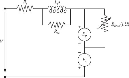
FIGURE 11.11 L-SRM single-phase circuit with propulsion (E_p) and suspension (E_S) pseudo-emfs.

The core losses occur in L-SRM both in the primary and in the secondary because the machine does not have a traveling field. A rather complete study of iron losses in rotary SRMs is offered in Ref. [3]. The iron core resistance R_iron in the equivalent circuit may thus be calculated or may be estimated from measurements during motion at constant current while R_ct refers to core losses due to current time variations (di/dt) during current control, mainly; R_ct may act even at standstill.

The multiphase equation of L-SRM may be simply written as

V a, b, c, d, .. = R S I a, b, c, d, .. + d ψ a , b , c , d , .. ( x , i a , b , c , d , .. ) d t (11.34)

$V_{a, b, c, d, ..} = R_{S} I_{a, b, c, d, ..} + \frac{d ψ_{a, b, c, d, ..} (x, i_{a, b, c, d, ..})}{d t} (11.34)$

F a, b, c, d, .. = \partial \partial x \int 0 i a, b, c, d, .. ψ a, b, c, d, .. (x, i a, b, c, d, ..) d i a, b, c, d, .. (11.35)

$F_{a, b, c, d, ..} = \frac{\partial}{\partial x} \int_{0}^{i_{a, b, c, d, ..}} ψ_{a, b, c, d, ..} (x, i_{a, b, c, d, ..}) d i_{a, b, c, d, ..} (11.35)$

As already mentioned, the flux linkage/current/position curve family is essential to calculating thrust F_x and normal force F_n. Its approximation is crucial for control system design, for example,

ψ (i, x) = a 1 (x) (1 - e - a 2 (x) i) + a 3 (x) i (11.36)

$ψ (i, x) = a_{1} (x) (1 - e^{- a_{2} (x) i}) + a_{3} (x) i (11.36)$

with

a 1, 2, 3 (x) = \sum k = 0 \infty A k 1, 2, 3 cos (2 π τ S x) (11.37)

$a_{1, 2, 3} (x) = \sum_{k = 0}^{\infty} A_{1, 2, 3}^{k} \cos (\frac{2 π}{τ_{S}} x) (11.37)$

ψ j = ψ s a t (1 - e - i j f j (x)); i j \geq 0 f j (x) = a 0 + \sum k = 1 3 a n cos (2 π τ s x - (i - 1) 2 π m); j = 1, 2, 3, 4 (for m = 4 phases) (11.38)

$\begin{array}{l} ψ_{j} = ψ_{s a t} (1 - e^{- i_{j} f_{j} (x)}); i_{j} \geq 0 \\ f_{j} (x) = a_{0} + \sum_{k = 1}^{3} a_{n} \cos (\frac{2 π}{τ_{s}} x - (i - 1) \frac{2 π}{m}); j = 1, 2, 3, 4 (for m = 4 phases) \end{array} (11.38)$

Approximations such as these are useful for rather high-fidelity curve fitting, allowing also analytical thrust and normal force expressions. However, for control design purposes two-piece linear approximations may be acceptable (Figure 11.12).

Images

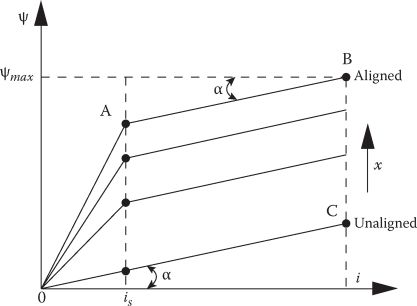
FIGURE 11.12 Simplified ψ(i)x curves.

ψ j = i j (L U + k U ( x - x o n ) i s τ p 2) ψ i = i j L U + k S ( x - x o n ) τ p 2; i \geq i s; i \leq i S (11.39)

$\begin{matrix} ψ_{j} = i_{j} (L_{U} + \frac{k_{U} (x - x_{o n})}{i_{s} \frac{τ_{p}}{2}}) \\ ψ_{i} = i_{j} L_{U} + \frac{k_{S} (x - x_{o n})}{\frac{τ_{p}}{2}}; i \geq i_{s} \end{matrix}; i \leq i_{S} (11.39)$

For this simplification, it suffices to perform 3D-FEM calculations, corresponding to points A, B, and C [9].

11.7 Small Signal Model of L-SRM

Let us revisit the voltage Equation 11.26 and add the motion equation (for propulsion only):

G m d U d t = F x - F L o a d - B U; d x d t = U; G m, mover mass (11.40)

$G_{m} \frac{d U}{d t} = F_{x} - F_{L o a d} - B U; \frac{d x}{d t} = U; G_{m}, mover mass (11.40)$

and neglect magnetic saturation to yield

F x = 1 2 \sum j = 1 3 (4) .. i 2 j \partial L j \partial x (11.41)

$F_{x} = \frac{1}{2} \sum_{j = 1}^{3 (4) ..} i_{j}^{2} \frac{\partial L_{j}}{\partial x} (11.41)$

Linearizing Equations 11.26 and 11.40 starts with

i = i 0 + Δ i; U = U 0 + Δ U; V = V 0 + Δ V; F l o a d = F L o + Δ F L o a d (11.42)

$i = i_{0} + Δ i; U = U_{0} + Δ U; V = V_{0} + Δ V; F_{l o a d} = F_{L o} + Δ F_{L o a d} (11.42)$

and yields

(s + 1 τ e) Δ i + k b L a v Δ U = Δ V L a v; R e = R S + \partial L \partial x U 0; L a v \approx ( L max + L min ) 2 - k b G m Δ i + (s + 1 τ m) Δ U = - Δ F l G m; τ e = L a v R e; k b = \partial L \partial x i 0; τ m = G m B (11.43)

$\begin{matrix} (s + \frac{1}{τ_{e}}) Δ i + \frac{k_{b}}{L_{a v}} Δ U = \frac{Δ V}{L_{a v}}; R_{e} = R_{S} + \frac{\partial L}{\partial x} U_{0}; L_{a v} \approx \frac{(L_{\max} + L_{\min})}{2} \\ - \frac{k_{b}}{G_{m}} Δ i + (s + \frac{1}{τ_{m}}) Δ U = - \frac{Δ F_{l}}{G_{m}}; τ_{e} = \frac{L_{a v}}{R_{e}}; k_{b} = \frac{\partial L}{\partial x} i_{0}; τ_{m} = \frac{G_{m}}{B} \end{matrix} (11.43)$

Note: The machine transient inductance is considered here as L_av (instead of L_t), while the phase inductance L varies linearly with position (x).

With ∆E=k_b∆U, the structural diagram of Equation 11.42 is presented in Figure 11.13.

The structural diagram in Figure 11.13 may be characterized as follows:

The equivalent resistance R_e includes the pseudo-emf influence and thus increases with speed; so the electric time constant τ_e decreases with speed.
The structural diagram is very similar to that of the dc series brush motor.
The equivalent time constants (τ₁ and τ₂) in the reduced structural diagram are dependent on i₀, U₀, ∂L/∂x, L_av, R_S.
The response of this second-order system is thus inherently stable; the response may be aperiodic or periodic but always attenuated.
The L-SRM operates as a motor for ∂L/∂x > 0 and as generator for ∂L/∂x < 0.

Images

FIGURE 11.13 L-SRM, per phase structural linear diagram (a) and its reduced form (b).

Example 11.2

Let us consider a three-phase L-SRM with L_min = 2 mH, L_max = 10 mH, and R_S = 0.2 Ω, which is operated at U₀ = 1 m/s and controlled at a constant current value l₀ over the entire x_{d wel} = τ_p/2 = 10 mm, which corresponds to equal pole and interpole primary lengths, for voltage V₀ = 42 Vdc.

Calculate

Current l₀, peak flux linkage Ψ_max, average thrust F_xav, and load force F_load at U₀ = 1 m/s.
For constant load and a 10% increase in average voltage V₀ (∆V = + 0.1 V₀) indicate the way for calculating the eigen values and current and speed transients using the small signal approach, with τ₁ = G_m/B = 3 s, B = 5.6 Ns.

Solution

1. The conducting time/phase t_on is

t o n = X d U 0 = 10 \times 10 - 3 1 = 0.01 s (11.44)

$t_{o n} = \frac{X_{d}}{U_{0}} = \frac{10 \times 10^{- 3}}{1} = 0.01 s (11.44)$

Using voltage equation yields (at constant speed)

V 0 t o n = R S I 0 t o n + (L max - L min) I 0 (11.45)

$V_{0} t_{o n} = R_{S} I_{0} t_{o n} + (L_{\max} - L_{\min}) I_{0} (11.45)$

I 0 = V 0 t o n R S t o n + ( L max - L min ) = 42 \times 0.01 0.2 \times 0.01 + ( 10 - 2 ) \times 10 - 3 = 42 A (11.46)

$I_{0} = \frac{V_{0} t_{o n}}{R_{S} t_{o n} + (L_{\max} - L_{\min})} = \frac{42 \times 0.01}{0.2 \times 0.01 + (10 - 2) \times 10^{- 3}} = 42 A (11.46)$

The average thrust F_xav/phase is in fact total average thrust as only one phase is active at any time:

F x a v = 1 2 i 20 \partial L \partial x = i 2 0 2 . ( L max - L min ) x d w e l l = 42 2 2 \cdot ( 10 - 2 ) 10 - 3 10 \times 10 - 3 = 705.6 N (11.47)

$F_{x a v} = \frac{1}{2} i_{0}^{2} \frac{\partial L}{\partial x} = \frac{i_{0}^{2}}{2} . \frac{(L_{\max} - L_{\min})}{x_{d w e l l}} = \frac{42^{2}}{2} \cdot \frac{(10 - 2) 10^{- 3}}{10 \times 10^{- 3}} = 705.6 N (11.47)$

Now the load force F_load is

F l o a d = F x a v - B U = 705.6 - 5.6 \times 1 = 700 N (11.48)

$F_{l o a d} = F_{x a v} - B U = 705.6 - 5.6 \times 1 = 700 N (11.48)$

2. The inductance variation may be written as

L (x) = L min + (L max - L min) x x d w e l l; 0 \leq x \leq x d w e l l (11.49)

$L (x) = L_{\min} + (L_{\max} - L_{\min}) \frac{x}{x_{d w e l l}}; 0 \leq x \leq x_{d w e l l} (11.49)$

So,

k b = \partial L \partial x I 0 = ( L max - L min ) x d w e l l \cdot I 0 = ( 10 - 2 ) \times 10 - 3 10 \times 10 - 3 \times 42 = 33.6 W b/m (11.50)

$k_{b} = \frac{\partial L}{\partial x} I_{0} = \frac{(L_{\max} - L_{\min})}{x_{d w e l l}} \cdot I_{0} = \frac{(10 - 2) \times 10^{- 3}}{10 \times 10^{- 3}} \times 42 = 33.6 W b/m (11.50)$

R e = R S + \partial L \partial x \cdot U 0 = 0.2 + ( 10 - 2 ) \times 10 - 3 10 \times 10 - 3 \times 1 = 0.2 + 0.8 = 1 Ω (11.51)

$R_{e} = R_{S} + \frac{\partial L}{\partial x} \cdot U_{0} = 0.2 + \frac{(10 - 2) \times 10^{- 3}}{10 \times 10^{- 3}} \times 1 = 0.2 + 0.8 = 1 Ω (11.51)$

The mover mass M_G = τ_m · B = 3 × 5.6 = 16.8 kg, and the equivalent electrical time constant

τ e = L a v R e = 6 \times 10 - 3 1 = 6 \times 10 - 3 S (11.52)

$τ_{e} = \frac{L_{a v}}{R_{e}} = \frac{6 \times 10^{- 3}}{1} = 6 \times 10^{- 3} S (11.52)$

The two small signal equations (11.43) write

(s + 1 6 \times 10 - 3) Δ i + 33.6 6 \times 10 - 3 Δ U = Δ V 6 \times 10 - 3 - 33.6 16.8 Δ i + (s + 1 3) Δ U = - Δ F L 16.8 (11.53)

$\begin{array}{l} (s + \frac{1}{6 \times 10^{- 3}}) Δ i + \frac{33.6}{6 \times 10^{- 3}} Δ U = \frac{Δ V}{6 \times 10^{- 3}} \\ - \frac{33.6}{16.8} Δ i + (s + \frac{1}{3}) Δ U = \frac{- Δ F_{L}}{16.8} \end{array} (11.53)$

Now solving the characteristic equation (11.53) for ∆V = 0.1V₀=4.2 V and ∆F_L = 0, the two eigen values s₁₂ are obtained. Once the eigen values are calculated (most probably in our case both are real and negative, say, −τ₁, −τ₂), the speed U is

U (t) = U 0 + Δ U (t) = U 0 + A 1 e - t τ 1 + A 2 e - t τ 2 + (U f i n a l - U 0) (11.54)

$U (t) = U_{0} + Δ U (t) = U_{0} + A_{1} e^{- \frac{t}{τ_{1}}} + A_{2} e^{- \frac{t}{τ_{2}}} + (U_{f i n a l} - U_{0}) (11.54)$

The new conducting time t_on′ (at the new steady-state speed) is

(V 0 + Δ V) t o n' = R S l 0 t o n' + (L max - L min) / 0 (11.55)

$(V_{0} + Δ V) t_{o n}' = R_{S} l_{0} t_{o n}' + (L_{\max} - L_{\min}) /_{0} (11.55)$

U f i n a l = U 0 \cdot t o n t o n ' (11.56)

$U_{f i n a l} = U_{0} \cdot \frac{t o n}{t_{o n}'} (11.56)$

Now also at t = 0, U = U₀ = 1 m/s, and (dU/dt)_t₌₀ = 0 and thus from (11.54), both A₁ and A₂ constants are obtained. The current variation Ai may be obtained from (11.42)

Δ i = (Δ U ( t ) τ m + d ( Δ U ( t ) ) d t) G m k b (11.57)

$Δ i = (\frac{Δ U (t)}{τ_{m}} + \frac{d (Δ U (t))}{d t}) \frac{G_{m}}{k_{b}} (11.57)$

As expected, the final speed increase is +10% as is voltage increase from constant load; and the current increases and then decreases to its initial value l₀, because the load is unchanged. The structural diagram with its reduced form may be used directly in the design of control system (Figure 11.14).

Images

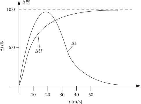
FIGURE 11.14 + 10% voltage step response at constant load (qualitative response). (After Krishnan, R., Switched Reluctance Motor Drives, CRC Press, Boca Raton, FL, 2001.)

11.8 Pwm Converters for L-SRMs

Typically, L-SRMs are supplied by unipolar currents per phase, and thus a two-switch per phase multiphase dc-dc converter with a front-end diode rectifier and capacitor filter constitutes the first option (Figure 11.15).

For typical hysteresis hard (fast) current control ± Vdc (with both switches on and off) is performed (Figure 11.4b); for soft (slower) current control +Vdc and zero voltage control is applied (Figure 11.14c). The minimum voltage rating of power devices is the dc link voltage. To provide equal RMS current in the power devices and the same average current in the freewheeling diodes, a distinct PWM strategy (different from those in Figure 11.14) is needed.

In essence, only one power switch is turned off to reduce the phase current, but the two power switches play this role one after the other. In an effort to reduce the number of power switches, quite a few alternative converter topologies have been proposed [3]. Among them, the C-dump converter stands out in terms of performance/cost Figure 11.15.

The total number of power switches is m + 1, and energy recovery when one (two) phase(s) is (are) active is secured from C-dump through T_r and L_r. There are five operation modes visible in Figure 11.16. The C-dump capacitor is calculated from its voltage variation ∆V₀ during T₁ turn off (from switch current ripple):

C d = ( 1 - d 1 ) I f c Δ V 0 (11.58)

$C_{d} = \frac{(1 - d_{1}) I}{f_{c} Δ V_{0}} (11.58)$

Where

d₁ is the minimum value T₁ of PWM index

I is average phase current

f_c is the switching frequency of current

The current ripple ∆i, for the interval, which corresponds to phase inductance variation ∆L (rotor position changes), is

Δ i = V d c \cdot d 1 f c \cdot L a v - I \cdot Δ L L a v (11.59)

$Δ i = \frac{V_{d c} \cdot d_{1}}{f_{c} \cdot L_{a v}} - \frac{I \cdot Δ L}{L_{a v}} (11.59)$

Images

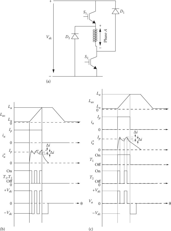
FIGURE 11.15 Two switches/phase dc–dc converter (a), hysteresis “hard” current control (b), and hysteresis “soft” current control (c). (After Krishnan, R., Switched Reluctance Motor Drives, CRC Press, Boca Raton, FL, 2001.)

Images

FIGURE 11.16 C-dump converter with energy recovery (a) and its main variable waveforms, (b). (After Krishnan, R., Switched Reluctance Motor Drives, CRC Press, Boca Raton, FL, 2001.)

Current ripple leads to torque pulsations and additional copper and iron losses. The minimum switching frequency is calculated by equating the duty cycle d₁ in (11.58) and in (11.59):

f c = V d c I \cdot Δ L + L \cdot Δ i + V d c \cdot C d \cdot S \cdot Δ V 0 (11.60)

$f_{c} = \frac{V_{d c}}{I \cdot Δ L + L \cdot Δ i + V_{d c} \cdot C_{d} \cdot S \cdot Δ V_{0}} (11.60)$

∆i and ∆V₀ are imposed in relative values for minimum I and L. We may continue with the design of the recovery inductance L_r (Figure 11.17), based on imposed ripple on the recovery current ∆i_r:

L r Δ i r = d 2 f c ( V 0 - V d c ) V 0 E p; E p = U \cdot I \partial L \partial x; U - speed (11.61)

$L_{r} Δ i_{r} = \frac{d_{2}}{f_{c}} \frac{(V_{0} - V_{d c})}{V_{0}} E_{p}; E_{p} = U \cdot I \frac{\partial L}{\partial x}; U - speed (11.61)$

where

I is the average phase current

E_p is the average pseudo emf per phase

Images

FIGURE 11.17 Variable dc link voltage buck-boost three-phase converter for L-SRM. (After Krishnan, R., Switched Reluctance Motor Drives, CRC Press, Boca Raton, FL, 2001.)

The phase voltage equation is such that

i (t) = V d c - E p R s (1 - e - t τ e) + i 0 e - t τ e; τ e = L ( x ) R S (11.62)

$i (t) = \frac{V_{d c} - E_{p}}{R_{s}} (1 - e^{- \frac{t}{τ_{e}}}) + i_{0} e^{- \frac{t}{τ_{e}}}; τ_{e} = \frac{L (x)}{R_{S}} (11.62)$

during t_on, when T₁ is on and T_r is off.

If R_S=0, the maximum and the minimum phase currents i(t) and i₀(t) are obtained from linear variations (hard commutation):

i (t) = i 0 (t) (V d c - E p L) t o n; i (t) = i 1 (t) - V 0 - V d c + E p L t o f f (11.63)

$i (t) = i_{0} (t) (\frac{V_{d c} - E_{p}}{L}) t_{o n}; i (t) = i_{1} (t) - \frac{V_{0} - V_{d c} + E_{p}}{L} t_{o f f} (11.63)$

t o n = d 1 1 f c; t o f f = ( 1 - d 1 ) f c (11.64)

$t_{o n} = d_{1} \frac{1}{f_{c}}; t_{o f f} = \frac{(1 - d_{1})}{f_{c}} (11.64)$

So the average PWM index d₁ is

d 1 = V 0 - V d c V 0 + E p V 0 (11.65)

$d_{1} = \frac{V_{0} - V_{d c}}{V_{0}} + \frac{E_{p}}{V_{0}} (11.65)$

Usually, the pseudo emf E_p is defined as equal to base voltage V_b. So at base speed U_b:

V 0 = V b = \partial L \partial x \cdot U b \cdot I b (11.66)

$V_{0} = V_{b} = \frac{\partial L}{\partial x} \cdot U_{b} \cdot I_{b} (11.66)$

Substituting in (11.63) yields

d 1 = 1 - V d c V b + U U b \cdot I I b; V d c V b = 0.7 - 0.8 (11.67)

$d_{1} = 1 - \frac{V_{d c}}{V_{b}} + \frac{U}{U_{b}} \cdot \frac{I}{I_{b}}; \frac{V_{d c}}{V_{b}} = 0.7 - 0.8 (11.67)$

As evident from (11.67), if V_dc/V_b = const., d₁ has to increase with speed U/U_b. Increasing V₀(V_b) for limited current limits the machine maximum speed. Adequate current (i_r) and voltage (V₀) control in the secondary circuit (L_r, C_d) leads to reasonable recovery current ripple ∆i_r [3]. Yet another variable dc link voltage buck-boost converter with m + 1 power switches is shown in Figure 11.17.

The switch T_c, diode D_c, inductor L, and capacitor C form the buck-boost part of the converter.

The machine phase voltage V_i may reach up to 2 V_dc (say, for wider constant power-speed range), but then the power switches have to be designed to three times V_dc for the scope. In the buck mode Vi < V_dc, and thus better low-speed performance may be obtained.

For more in L-SRM converters, see Ref. [3], Chapter 4.

11.9 Design Methodology by Example

Let us develop an electromagnetic design methodology for an L-SRM with specifications as given in the following:

Rated thrust to base speed: F_xn=400 N

Base speed U_b=2.4 m/s

DC link voltage V_dc = V₀ = 300 Vdc
Number of phases m=3 (6 coils in all)
Topology: tubular
Travel length: 1 m
Free acceleration to U_b length ≤0.2 m
Flux/current/position curves: piece-wise linear

First, a thrust density by f_xn = 1.6 N/cm² for the stroke length l_stroke = τ_p/2 = 15 mm and the airgap g = 0.3 mm is adopted. To retain enough time to turn off the active phase before producing drag force, we choose

x 0 - x u l s t r o k e = 0.8 (11.68)

$\frac{x_{0} - x_{u}}{l_{s t r o k e}} = 0.8 (11.68)$

From (11.23), we my calculate (with R_S = 0) the maximum flux linkage in the phase ψ_b:

ψ b = V d c U \cdot 0.8 \cdot l s t r o k e = 300 2.4 \times 0.8 \times 15 \times 10 - 3 = 1.5 Wb (11.69)

$ψ_{b} = \frac{V_{d c}}{U} \cdot 0.8 \cdot l_{s t r o k e} = \frac{300}{2.4} \times 0.8 \times 15 \times 10^{- 3} = 1.5 Wb (11.69)$

With equal primary slot and pole span, the primary (pole) length is b_p = l_stroke = 15 mm. The secondary slot pitch τ_s is thus

τ S = 3 l s t r o k e = 45 mm (11.70)

$τ_{S} = 3 l_{s t r o k e} = 45 mm (11.70)$

The maximum thrust (current) is produced when (Figure 11.18) L_S=L_u (unaligned).

W m e c k s a f e \approx ψ' 0 (x 0 - x u l s t r o k e) I b - ψ ' 2 0 2 L a u; k s a f e < 1; ψ' 0 = ψ b - L S \cdot I b (11.71)

$\frac{W_{m e c}}{k_{s a f e}} \approx {ψ^{'}}_{0} (\frac{x_{0} - x_{u}}{l_{s t r o k e}}) I_{b} - \frac{{ψ^{'}}_{0}^{2}}{2 L_{a u}}; k_{s a f e} < 1; {ψ^{'}}_{0} = ψ_{b} - L_{S} \cdot I_{b} (11.71)$

k_safe is a safety factor.

Equation 11.71 may be used as verification after the design is done. At this stage, we can calculate the L-SRM diameter at airgap D_pi, as there are only two coils/phase and only one active phase at a time:

F x n = π \cdot D p i \cdot 2 (2 l s t r o k e) \cdot f x n D p i = 400 π \times 4 \times 2 \times 15 \times 10 - 3 \times 1.6 \times 104 = 0.0664 m (11.72)

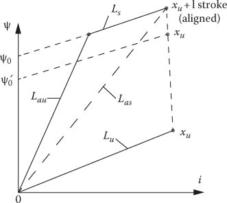
$\begin{array}{l} F_{x n} = π \cdot D_{p i} \cdot 2 (2 l_{s t r o k e}) \cdot f_{x n} \\ D_{p i} = \frac{400}{π \times 4 \times 2 \times 15 \times 10^{- 3} \times 1.6 \times 104} = 0.0664 m \end{array} (11.72)$

Images

FIGURE 11.18 Simplified ψ(i)x curves.

Let us allow for maximum of airgap flux density in the aligned position of a phase to be B_b = 1.4 T.

The maximum flux linkage in the two coils per phase in series ψ_b is

ψ b = 2 \cdot B b \cdot b b \cdot π \cdot D p i \cdot W C; k d = x 0 - x u l s t r o k e = 0.8 (11.73)

$ψ_{b} = 2 \cdot B_{b} \cdot b_{b} \cdot π \cdot D_{p i} \cdot W_{C}; k_{d} = \frac{x_{0} - x_{u}}{l_{s t r o k e}} = 0.8 (11.73)$

W_C is the turn/coil

B b \cdot W C = 1.5 2 \times 0.015 \times π \times 0.0664 = 239 T \cdot turns (11.74)

$B_{b} \cdot W_{C} = \frac{1.5}{2 \times 0.015 \times π \times 0.0664} = 239 T \cdot turns (11.74)$

The unaligned L_u and aligned L_au inductances per phase are

L u = 2 P m u \cdot W 2 C; L a u = 2 P m a \cdot W 2 C (11.75)

$L_{u} = 2 P_{m u} \cdot W_{C}^{2}; L_{a u} = 2 P_{m a} \cdot W_{C}^{2} (11.75)$

P_mu, P_ma magnetic permeances per coil in unaligned and aligned position (see Figure 11.19 per phase A)—unsaturated:

P m a \approx μ 0 \cdot π \cdot D S i \cdot b p 2 g (11.76)

$P_{m a} \approx \frac{μ_{0} \cdot π \cdot D_{S i} \cdot b_{p}}{2 g} (11.76)$

For saturated conditions in aligned position,

L a S = 2 \cdot P m a s \cdot W 2 C; P m a s = P m a ( 1 + k S ); k S — saturation factor . (11.77)

$L_{a S} = 2 \cdot P_{m a s} \cdot W_{C}^{2}; P_{m a s} = \frac{P_{m a}}{(1 + k_{S})}; k_{S} — saturation factor . (11.77)$

Images

FIGURE 11.19 Tubular three-phase L-SRM.

Now with B_b = 1.4 T from (11.74), the number of turns per coil W_C is

W C = W C B b B b = 239 1.4 \approx 170 turns/coil (11.78)

$W_{C} = \frac{W_{C} B_{b}}{B_{b}} = \frac{239}{1.4} \approx 170 turns/coil (11.78)$

So the unsaturated aligned position inductance yields

L a u = 2 μ 0 π D p i b p W 2 C 2 g = 2 \times 1.1256 \times 10 - 6 \times π \times 0.0664 \times 0.015 \times 170 2 2 \times 0.3 \times 10 - 3 = 0.37884 H (11.79)

$L_{a u} = \frac{2 μ_{0} π D_{p i} b_{p} W_{C}^{2}}{2 g} = \frac{2 \times 1.1256 \times 10^{- 6} \times π \times 0.0664 \times 0.015 \times 170^{2}}{2 \times 0.3 \times 10^{- 3}} = 0.37884 H (11.79)$

From field calculations (analytical [3] or 2D-FEM), the unaligned inductance L_u is L_u=L_au/10 = 0.03784 H. With k_safe = 0.75, k_d=0.8, from (11.71) we may directly calculate the base (flat-top) phase current I_b as

W m e c = F x a v \cdot l s t r o k e = 400 \times 15 \times 10 - 3 = 6 J (11.80)

$W_{m e c} = F_{x a v} \cdot l_{s t r o k e} = 400 \times 15 \times 10^{- 3} = 6 J (11.80)$

6 0.75 \approx (1.5 - 0.03784 \cdot I b) 0.8 \cdot I b - ( 1.5 - 0.03784 \cdot I b ) 2 0.8 2 2 \times 0.03784 I b \approx 8.35 A (11.81)

$\begin{matrix} \frac{6}{0.75} \approx (1.5 - 0.03784 \cdot I_{b}) 0.8 \cdot I_{b} - \frac{{(1.5 - 0.03784 \cdot I_{b})}^{2} {0.8}^{2}}{2 \times 0.03784} \\ I_{b} \approx 8.35 A \end{matrix} (11.81)$

The saturated inductance L_as (Figure 11.18) is thus obtained from

ψ b = L a s \cdot I b \cdot k d; L a s = 1.5 8.25 \times 0.8 = 0.22 H (11.82)

$ψ_{b} = L_{a s} \cdot I_{b} \cdot k_{d}; L_{a s} = \frac{1.5}{8.25 \times 0.8} = 0.22 H (11.82)$

The RMS current/phase (I_b)_RMS is approximately

(I b) R M S = I b 3 - \sqrt = 8.25 3 - \sqrt = 4.768 A (11.83)

${(I_{b})}_{R M S} = \frac{I_{b}}{\sqrt{3}} = \frac{8.25}{\sqrt{3}} = 4.768 A (11.83)$

With J_{Co RMS} = 3 A/mm² and slot filling factor k_sfill = 0.5, the slot area of primary A_slotp is

A s l o t p = I b R M S \cdot W C J C o R M S \cdot k s f i l l = 4.768 \times 170 3 \times 0.5 = 540 mm 2 (11.84)

$A_{s l o t p} = \frac{I_{b R M S} \cdot W_{C}}{J_{C o R M S} \cdot k_{s f i l l}} = \frac{4.768 \times 170}{3 \times 0.5} = 540 {mm}^{2} (11.84)$

But the slot b_sp = b_p = 15 mm and thus the slot height is

h s p = A s l o t p b s p = 540 15 = 36 mm (11.85)

$h_{s p} = \frac{A_{s l o t p}}{b_{s p}} = \frac{540}{15} = 36 mm (11.85)$

The secondary tooth height (to reduce flux fringing) h_ss = 20 g = 20 × 0.3 = 6 mm.

The saturation factor k_S is

k S = L a u L a s - 1 = 0.3784 0.22 - 1 = 0.72 (11.86)

$k_{S} = \frac{L_{a u}}{L_{a s}} - 1 = \frac{0.3784}{0.22} - 1 = 0.72 (11.86)$

There is enough space for reducing the primary and secondary back iron to reach this value of k_S. A routine utilization of Ampere’s law along the field line as in Figure 11.19 will yield k_S for B_b = 1.4 T. It is imperative to get B_b = 1.4 T for aligned position for W_C · I_b = 170 × 8.4768 = 1441.056; otherwise, the rated thrust will not be obtained. The copper losses are

P C o n = 3 I 2 b R M S \cdot R S (11.87)

$P_{C o n} = 3 I_{b R M S}^{2} \cdot R_{S} (11.87)$

with

R S = 2 ρ C o π (D P i + h s p) W C I b R M S J C O R M S = 2.21 \times 10 - 8 \times π \times (0.064) \times 170 4.788 \times 3 \times 10 - 6 = 0.8866 Ω (11.88)

$\begin{array}{l} R_{S} = 2 ρ_{C o} π (D_{P i} + h_{s p}) \frac{W_{C}}{I_{b R M S}} J_{C O R M S} \\ = 2.21 \times 10^{- 8} \times π \times (0.064) \times \frac{170}{4.788} \times 3 \times 10^{- 6} = 0.8866 Ω \end{array} (11.88)$

So,

P C o n \approx 3 \times 0.8866 \times 4.768 2 = 60.46 W (11.89)

$P_{C o n} \approx 3 \times 0.8866 \times {4.768}^{2} = 60.46 W (11.89)$

The frequency f_n is

f n = U b τ s = 2.4 45 \times 10 - 3 = 53.33 Hz (11.90)

$f_{n} = \frac{U_{b}}{τ_{s}} = \frac{2.4}{45 \times 10^{- 3}} = 53.33 Hz (11.90)$

The approximate weight of primary is

G p \approx π ( ( D p i + 2 h s y + 2 h c p ) 2 - D 2 P i ) 4 \cdot 13 \cdot b p \cdot γ i + c = π ( ( 66.4 + 2 \times 36 + 2 \times 10 ) 2 - 66.4 2 ) 4 \times 10 - 6 \times 13 \times 15 \times 10 - 3 \times 8200 = 25.96 kg (11.91)

$\begin{matrix} G_{p} \approx \frac{π ({(D_{p i} + 2 h_{s y} + 2 h_{c p})}^{2} - D_{P i}^{2})}{4} \cdot 13 \cdot b_{p} \cdot γ_{i + c} \\ = \frac{π ({(66.4 + 2 \times 36 + 2 \times 10)}^{2} - {66.4}^{2})}{4} \times 10^{- 6} \times 13 \times 15 \times 10^{- 3} \times 8200 = 25.96 kg \end{matrix} (11.91)$

With a thrust of 400 N, the ideal acceleration of primary a_i_max is

a i max = F x a G p = 400 25.96 = 15.408 m / s 2 (11.92)

$a_{i \max} = \frac{F_{x a}}{G_{p}} = \frac{400}{25.96} = 15.408 m / s^{2} (11.92)$

The ideal acceleration travel l_travel to U_b=2.4 m/s from standstill is

l t r a v e l = U 2 b 2 a = 2.4 2 2 \times 15.408 = 0.187 m < 0.2 m (11.93)

$l_{t r a v e l} = \frac{U_{b}^{2}}{2 a} = \frac{{2.4}^{2}}{2 \times 15.408} = 0.187 m < 0.2 m (11.93)$

So the ideal acceleration to full speed may be accomplished under 0.2 m of travel out of the total travel of 1 m.

The efficiency may be calculated as

η n = P m e c P m e c + P C o m + P i r o n + P m e c (11.94)

$η_{n} = \frac{P_{m e c}}{P_{m e c} + P_{C o m} + P_{i r o n} + P_{m e c}} (11.94)$

With about 60% iron in the primary (15 kg) and 5 kg in the secondary and 2.5 W/kg iron losses and 10 W mechanical losses, the total efficiency is

η n = 400 \times 2.4 960 + 60.46 + 20 \times 2.5 + 10 = 0.888 (11.95)

$η_{n} = \frac{400 \times 2.4}{960 + 60.46 + 20 \times 2.5 + 10} = 0.888 (11.95)$

Note: At this speed (2.4 m/s), the designed L-SRM is better than the LIM for same size and output in terms of efficiency; in terms of converter kVA, it is about the same (cos φ of an LIM is about 0.4 ÷ 0.5). A distinct design for a ship elevator of 55,000 N with multimodular, flat, double-sided, four-phase L-SRMs with active movers is described in Ref. [10] and could be a valuable guide of L-SRM potential.

Efforts to reduce undesired high normal force in single-sided flat L-SRM by pole shaping design are presented in Ref. [11], while separated-phase tubular topologies of L-SRM are designed in Ref. [12].

11.9.1 L-SRM CONTROL

By L-SRM control, we mean position or speed or thrust close-loop regulation.

Instantaneous current close-loop control is, in general, implicit. In L-SRM control, we may suppose that

Position sensing (by linear encoders or resolvers) is available
Motion-sensorless control is performed (in general) for speed and (or) thrust control

In view of the complexity of the flux/current/position and thrust/current/position curve families, the position, speed, or thrust control is rather nonlinear.

The linearized second-order structural diagram (11.13b) may be used for a preliminary design of, first, the current regulator and then the speed regulator (Figure 11.20; this design may be considered as preliminary. Thorough verifications of stability and performance of current and speed control in extreme conditions of thrust perturbations and machine parameter detuning are then required.

The generic control system in Figure 11.20 includes the following:

A fast phase current regulator with limiter (to avoid trespassing of maximum voltage available in the converter and for current fast protection).
1–2 kHz critical frequency with a damping factor ξ = 0.6–0.7.
A mildly fast speed regulator with a critical frequency around 100 Hz or more and, again, a damping factor ξ = 0.6–0.75.
A proportional (if any) position controller for a positioning application.
Other more robust controllers may be applied.

Images

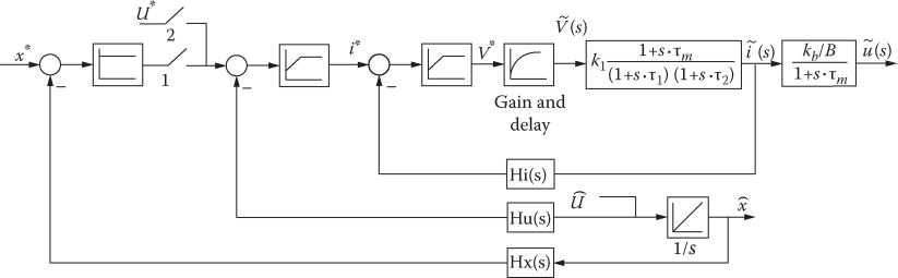
FIGURE 11.20 Generic cascaded position, speed, and current control; one phase in terms of current control is shown. (After Lim, H.S. et al., IEEE Trans,, IE-55(2), 534, 2008.)

For details of current and speed regulator design, see Ref. [3]. Once the preliminary design of current speed and position regulators is done, a more complete view of the current control may be obtained, by establishing the waveforms of phase reference currents for each phase so as to produce the required dynamic response and to exhibit low thrust pulsations and thus avoid noise and vibrations. Reference current waveforms for a given average torque and speed (to fulfill, in the presence of magnetic saturation) are not easy to find.

However, if magnetic saturation is not considered, the situation simplifies to some extent as the thrust of phase k is

F x k = 1 2 g k (x) \cdot i 2 k; g k (x) = \partial L k \partial x (11.96)

$F_{x k} = \frac{1}{2} g_{k} (x) \cdot i_{k}^{2}; g_{k} (x) = \frac{\partial L_{k}}{\partial x} (11.96)$

For a four-phase L-SRM, the phase inductances L_a,b,c,d vary with position (magnetic saturation is absent or constant) as in Figure 11.21 [4].

As seen in Figure 11.20, the waveforms of the current should be obtained by reversing (11.96):

i * k (x) = 2 F * x k g k ( x ) - - - - - \sqrt (11.97)

$i_{k}^{*} (x) = \sqrt{\frac{2 F_{x k}^{*}}{g_{k} (x)}} (11.97)$

Images

FIGURE 11.21 Inductances (a, b, c, d) (a), thurst (Fx) (b), and dL/dx (c) versus position for a four-phase L-SRM. (After Lim, H.S. et al., IEEE Trans., IE-55(2), 534, 2008.)

But, more than that, the reference thrust F∗xk $F_{x k}^{*}$ of each phase should be modulated with a function f_k(x) such that the total reference thrust is obtained always with most efficient (in thrust) phases:

F * x = \sum F * x \cdot f x (k); \sum k = a, b, c, d f k = 1 (11.98)

$F_{x}^{*} = \sum F_{x}^{*} \cdot f_{x} (k); \sum_{k = a, b, c, d} f_{k} = 1 (11.98)$

f_x is called force distribution factor (FDF) [4], and its function choice is a matter of experience or trial and error, to minimize, again, the thrust pulsations with mover position in a feed forward manner.

A typical result with such an FDF system is shown in Figure 11.21 [4].

The control system in such a case may be defined as in Figure 11.22.

Though f_k(x) and g(k) are a priori functions of mover position, the design of position, speed, and current regulator for a single phase with constant equivalent current could be a good start for more involved investigations. Digital simulations and experiments for critical dynamic operation modes will then validate the simplified regulator designs. Such dynamic simulation results [4] show good performance (Figures 11.23 and 11.24).

Controlled power-speed region extension control may be obtained by just changing FDF, that is, f_k(x) functions with speed (and, evenly, with reference total thrust F∗x $F_{x}^{*}$ ). In an effort to reduce the off- and on-line computation effort, very visible in Figure 11.22, direct average thrust control may be attempted [17]. The average thrust may be estimated by starting with phase flux estimation:

d d t Ψ k = V k - R S I k; k = a, b, c, d \dots (11.99)

$\frac{d}{d t} Ψ_{k} = V_{k} - R_{S} I_{k}; k = a, b, c, d \dots (11.99)$

Images

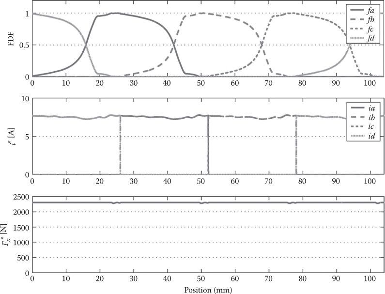
FIGURE 11.22 Thrust control with FDF thrust reference at U=−0.5 m/s and advance phase excitation by 2 mm. (After Lim, H.S. et al., IEEE Trans., IE-55(2), 534, 2008.)

Images

FIGURE 11.23 Four-phase L-SRM control: (a) structural diagram, (b) thrust division between phases and current control. (After Lim, H.S. et al., IEEE Trans., IE-55(2), 534, 2008.)

Images

FIGURE 11.24 Position and speed repetitive response (flat-top speed is + 0.33 m/s). (After Lim, H.S. et al., IEEE Trans., IE-55(2), 534, 2008.)

The mechanical energy W_mec per cycle (from zero to zero current per phase) is

W m e c = \int d ψ d t i \cdot d t = \int x o n x o f f \partial W ' m \partial x \cdot d x = \int x o n x o f f \int 0 i \partial ψ k ( x , i ) \partial x \cdot d i \cdot d x (11.100)

$W_{m e c} = \int \frac{d ψ}{d t} i \cdot d t = \int_{x o n}^{x o f f} \frac{\partial {W^{'}}_{m}}{\partial x} \cdot d x = \int_{x o n}^{x o f f} \int_{0}^{i} \frac{\partial ψ_{k} (x, i)}{\partial x} \cdot d i \cdot d x (11.100)$

This integral should be reset to zero after the current reaches zero and thus the magnetization—demagnetization energy portions per phase cancel each other, and the average thrust of the machine per stroke is

F x a v = m W m e c l s t r o k e (11.101)

$F_{x a v} = m \frac{W_{m e c}}{l_{s t r o k e}} (11.101)$

m is the number of phases

The average torque estimator is illustrated in Figure 11.25a.

The generic direct average thrust control in Figure 11.25 may be characterized as follows:

It uses an average thrust/phase estimator based on a flux calculator from the voltage model: integral offset, converter nonlinearities, and phase resistance correction are all needed for good operation down to low speed.
The average thrust may be estimated for each phase and added for faster average thrust control, as anyway current regulators are in general needed for all phases.
The off-line computation effort is concentrated (Figure 11.25) to calculate, for given average thrust F_x, dc voltage V_dc, mover position x and speed U, the flat average top current level I₀, the turn on position x_on (advanced at higher speeds), and the commutation (turn off) position x_co.
Also, if the thrust has to be negative (regenerative braking) the off-line calibrator sets x_on and x_co at their proper values (into the negative inductance slope region).
It has to be conceded that for an acceptable control of L-SRM, even with a position feedback sensor, both the off-line and the on-line computer effort is more demanding than for LIMs or LSMs as will be seen in further chapters on L-PMSMs; however, the absence of PMs and the motor ruggedness and lower initial costs make L-SRM a strong candidate in cost- and temperature-sensitive applications.

Images

FIGURE 11.25 Direct average torque control of L-SRM: (a) average torque estimation and (b) generic control (c) typical waveforms of current, voltage, flux linkage and energy.

Images

11.9.2 Note on Motion-Sensorless Control

Motion-sensorless control of L-SRMs is very similar to that of their rotary counterparts [3]. However, the absolute position estimation needs at least one marked position in the secondary (fixed part, in general) to detect a reference signal. For speed control, however, only relative position is required.

Other than these remarks, the rich body of knowledge of sensorless control of rotary SRM may be adapted for linear motion control by L-SRM. An exemplary investigation, to follow, is given in Ref. [13].

11.10 Summary

L-SRMs are counterparts of rotary SRMs.
The combinations of stator N_S and rotor N_R poles typical to rotary SRMs have to translate into ratios of active primary to passive secondary saliency period (τ_p/τ_s).
L-SRMs may be flat, single sided, double sided, and tubular.
As the normal force F_n to thrust F_x ratio in flat single-sided L-SRMs tends to be larger than 10/1, either the normal force is controlled for magnetic levitation or double-sided flat or tubular topologies are to be used. Recent new dual primary topologies reduce the F_n/F_x ratio considerably [18].
As for rotary machines, longitudinal and transverse flux topologies are feasible; transverse topologies are in general free of longitudinal end static effects, and thus with 3(6) or 4(8) primary pole small L-SRMs such configurations for 3(4) phase operation are recommended.
A typical, single (secondary) saliency topology with 5, 6, 7 phases and two-level bipolar current control, where m_F phases produce the “excitation” and the other m − m_F phases are thrust phases, is also introduced as potentially it may yield good thrust and normal force density for good efficiency and reasonable peak kVA ratings in the multiphase inverter topology.
To illustrate the operation principle, a simple U core primary single coil with I-secondary is investigated for thrust, normal force, and losses/thrust performance. The attraction of the laminated secondary to the primary, when the latter is supplied, and the typical coenergy variation with position (x and g-airgap) are the basis for thrust and normal force production in L-SRM. In a numerical example, 2.6 N/cm² of thrust, 87 N/cm² of normal force, and 0.9 N/W of copper losses are typical performance indexes for L-SRM.
The instantaneous thrust calculation from the coenergy (Fx=−(∂W′m/∂x)i=const.) $(F_{x} = - {(\partial {W^{'}}_{m} / \partial x)}_{i = c o n s t .})$ requires the flux linkage/current/position family of curves, which may be calculated via complex magnetic circuit or FEM models or measured (from standstill current-decay tests).
Due to magnetic saturation, the thrust/position curve for constant current is not a horizontal line and thus commutation phases are added—there may be notable thrust pulsations with flat-top current control in three- or even in four-phase L-SRMs.
But magnetic saturation reduces the transient (commutation) inductance (L′ = L + i∂L/∂i) and thus allows higher speeds.
From the flux/current/position, ψ/i/x, family of curves, the average mechanical energy per energy cycle/phase may be determined W_mec = F_xav · l_stroke(lstroke ≈ τ_p/2). A part of energy W_mag is returned to the dc link through the PWM converter that supplies each phase.
The ratio η_ec = W_mec/(W_mec + W_mag) is called the energy cycle conversion ratio and it is 0.5 for nonsaturated L-SRM and 0.6−0.67 for saturated conditions. A low η_ec is an indication of high kVA rating requirements from the PWM converter supply. In general, the peak kVA of the converter is larger than for most ac linear motors.
As the thrust sign (for motoring or generating) does not depend on current polarity, homopolar current is in general supplied to L-SRM phases.
The phase magnetic coupling is rather small in L-SRMs, which is good for fault tolerance but not so good for thrust density.
The state space equations contain phase voltage equations and the equations of motions.
The phase voltage equations contain a pseudo-emf
<unnumbered_display_equation/>

$(E = i \partial L ( x , i , g ) \partial x d x d t + i \partial L ( x , i , g ) \partial g d g d t),$ $(E = i \frac{\partial L (x, i, g)}{\partial x} \frac{d x}{d t} + i \frac{\partial L (x, i, g)}{\partial g} \frac{d g}{d t}),$

which is related to linear (along x) and vertical (along g) motions: however, the thrust may be calculated from F_x = (i²/2)(∂L/∂x) only in the absence of magnetic saturation (all ψ/i/x curves are linear); otherwise, the coenergy formula has to be used (Fx=−(∂W′m/∂x)i=const.) $(F_{x} = - {(\partial {W^{'}}_{m} / \partial x)}_{i = c o n s t .})$ .
As the L-SRM is not a traveling field machine, there are core losses both in the primary and in the secondary; they have to be carefully assessed in any realistic efficiency calculation attempt.
For linear piece-wise ψ/i/x curves (Figure 11.12), with state space equations linearization, a second-order structural diagram for transients, typical to series dc excited brush motor, are obtained. This result helps notably in the design of the current and speed close-loop regulators for L-SRM.
From a myriad [3] of unipolar current multiphase dc–dc converters suitable for L-SRMs, only the one with two power switches per phase (2 m switches in general) and the C-dump converter with m + 1 power switches are introduced and characterized here as very practical for the scope. An analytical design methodology based on linear-wise ψ/i/x curve (magnetic saturation not considered) has been developed in this chapter via a numerical example: the design yields also all circuit parameters tuned for close-loop current and speed regulators. For a 400 N, 2.4 m/s, tubular L-SRM case study, a total efficiency of 0.888 is obtained for an active primary of 26 kg; an ideal acceleration of active primary mover of 15 m/s² is obtained, which allows for acceleration to 2.4 m/s within 0.2 m, which may be enough for many short travel transportation jobs in industrial applications.
The control of L-SRM is approached first through the cascaded—current, speed, position—strategy that makes use of the linearized second-order model of L-SRM for control design.
The “force distribution factor” (FDF) f_k dependent on ∂L/∂x, when supplied for a nonsaturated four-phase L-SRM to produce the required reference current waveforms that reduce the thrust pulsation to less than 10%, is good enough in many servo applications.
Positioning steady-state error of 3.5 µm has been claimed with a rather involved computer intensive control of three-phase L-SRM [14,15].
In an effort to reduce the off- and on-line computation effort, a direct average thrust control system is presented in some detail.
A note on motion-sensorless control sends to the sensorless control of rotary SRM [3] wherefrom a lot can be used for L-SRMs.
As the use of PMs in electromagnetic devices increases (especially in automotive and wind and small hydro sectors), the SRMs and especially L-SRMs may become more competitive due to their simplicity, ruggedness, and low enough initial system costs.

References

1. T.J.E. Miller, Switched Reluctance Motors and Their Control, Magna Physics Publishing, Oxford, U.K., 1993.

2. I. Boldea and S.A. Nasar, Linear Electric Actuators and Generators, Cambridge University Press, Cambridge, U.K., 1997.

3. R. Krishnan, Switched Reluctance Motor Drives, CRC Press, Boca Raton, FL, 2001.

4. H.S. Lim, R. Krishnan, and N.S. Lobo, Design and control of linear propulsion system for an elevator using linear switched reluctance motor drives, IEEE Trans., IE-55(2), 2008, 534–542.

5. K.B. Saad, M. Benrejeb, and P. Brochet, One two control methods for smoothing the linear tubular switched reluctance stepping motor position, Record of LDIA-2007.

6. I.D. Law, A. Chertok, and T.A. Lipo, Design and performance of the field regulated reluctance machine, Record of IEEE-IAS, 1992, vol. 1, Houston, TX, pp. 234–241.

7. I. Boldea, Reluctance Synchronous Machines and Drives, Chapter 2, Oxford University Press, U.K., 1996.

8. I. Boldea, Variable Speed Generators, Chapter 9, CRC Press, Taylor & Francis, Boca Raton, FL, 2006.

9. A. Radun, Design considerations on SRMs, Record of IEEE-IAS, 1994.

10. H.S. Lim, Design and control of a linear propulsion system for an elevator using L-SRM drives, IEEE Trans., IE-55(2), 2008, 534–542.

11. E. Santo, M.R. Calado, and C.M. Cabrita, Influence of pole shape in linear switched reluctance actuator performance, Record of LDIA, 2007.

12. W. Missaoui, L. El Ambraoni Ouni, F. Gillon, M. Benrejeb, and P. Brochet, Comparisons of magnetic behavior of SR and PM tubular linear three-phase synchronous linear motors, Record of LDIA, 2007.

13. G. Pasquesoone and I. Husain, Position estimation at starting and lower speed in 3 phase SRMs using pulse injection and two thresholds, Record of IEEE-ECCE, 2010, pp. 2660–2666.

14. W.-C. Gan, N.C. Cheung, and L. Qiu, Position control of linear SRMs for high precision applications, IEEE Trans., IA-39(5), 2003, 1350–1362.

15. S.H. Lee and Y.S. Baek, Contact free switched reluctance linear actuator for precision stage, IEEE Trans., Mag-40(4), 2004, 3075–3077.

16. G. Baoming, A.T. de Almeida, and F. Ferreira, Design of transverse flux linear switched reluctance motor, IEEE Trans., Mag-45(1), 2009, 113–119.

17. R.B. Inderka and R.W. de Doncker, Simple average torque estimation for control of SRMs, Record of EPE-PEMC, 2000, vol. 5, Kosice, Slovakia, pp. 176–181.

18. W. Wang, C.H. Lin, and B. Fahimi, Comparative analysis of double stator switched reluctance machine and PSMS, Record of IEEE-ISIE, 2012.

..................Content has been hidden....................

You can't read the all page of ebook, please click here login for view all page.

Table of Contents for Chapter 11 Linear Switched Reluctance Motors (L-SRM): Modeling, Design, and Control

Create new playlist

Sign In

Sign Up

Modeling, Design, and Control

Table of Contents for
Chapter 11 Linear Switched Reluctance Motors (L-SRM): Modeling, Design, and Control