Chapter 12 Flat Linear Permanent Magnet Synchronous Motors

Search in book...
Toggle Font Controls
Create new playlist

Name your new playlist

Playlist description (optional)
Sign In

Email address

Password

Forgot Password?

or

Continue with Facebook

Continue with Google
Sign Up

Full Name

Email address

Confirm Email Address

Password

or

Continue with Facebook

Continue with Google

By flat linear permanent magnet synchronous motors (F-LPMSM), we mean here single- or double-sided, short mover or long stator three-phase ac-fed primary and long (stator) or short (mover) secondary configurations, with sinusoidal or trapezoidal emf or current waveform control. Both distributed (q > 1) and tooth-wound three-phase windings in iron or air-core primaries are considered. The tubular linear PM motors (T-LPMSMs) are treated in a separate chapter as their design and control is related to the rather short travel length (below 2–3 m). Linear PM brushless motors with variable reluctance short (mover) or long (stator) secondary and PM primaries that contain both the PMs and three-phase ac windings will also be treated separately under the name of pulse linear PM brushless motors (P-LPMBM).

The F-LPMSM may be applied, in the long iron-core primary (stator) and short PM mover configuration, for industrial urban and interurban transportation. Short (mover) primary and long PM-secondary (stator) F-LPMSM configurations are used in short travel (a few meters) both in single-sided versions (as MAGLEV carriers, especially) and in double-sided PM-secondary (tube) versions, when the normal force on the short primary (mover) is to be zero, in order to avoid noise, vibration, and large stray PM magnetic fields.

In what follows, we will first discuss practical topologies, analytical (technical) and finite element method (FEM) field theories for F-LPMSMs, cogging force computation and reduction, circuit parameters, and circuit models for dynamic and field oriented control (FOC) and direct thrust and flux control (DTFC); then a design methodology is introduced by numerical example.

12.1 A Few Practical Topologies

Though there are many “novel” topologies for F-LPSM, only a few are representative and practical:

Single-sided type (Figure 12.1a,b, and d)
Double-sided type (Figure 12.1c and f)
Short PM secondary (mover) type (Figure 12.1a and d)
Short ac primary (mover) type (Figure 12.1c,e,f, and g)
Distributed (q = 1 slot/pole/phase) three-phase ac winding (Figure 12.1a through d)
Concentrated (tooth-wound) three-phase winding (Figure 12.1e,f, and g)
Iron-tooth primary core (Figure 12.1a through f)
Air-core primary (three-phase) (Figure 12.1c)
With surface PM secondary (Figure 12.1a,c through g)
With Halbach array PMs secondary (Figure 12.1b)
With four sides (Figure 12.1g)

An investigation of these configurations reveals the following:

The cable-coil q = 1, single layer, three-phase winding (Figure 12.1a and d) is easy to install along track, with a fixed primary (stator), but it requires open slots, and thus the airgap should be about the size of the slot openings (or less) to allow small emf harmonics and low enough cogging force. The configuration would be typical for urban or interurban MAGLEVs with an active guideway (airgap from 6 to 10 mm).
The Halbach PM array secondary (Figure 12.1b) leads to less emf ripple, higher thrust and lower cogging (zero current) force, and thinner secondary back core; it may be used with both PM mover or mild length (travel) PM stator.
The double-sided PM-secondary stator with air-core primary (mover) is typical for industrial linear motor automation when the cogging force has to be small (less than 1%), and the stray PM fields still have to be limited.
The hybrid PM + dc coil secondary mover configuration (Figure 12.1d) is typical for active guideway (primary) MAGLEVs.
The single-sided 6 slot/8 PM pole configuration (Figure 12.1e) is just an example of tooth-wound three-phase winding; to reduce cogging force, the PM span per pole pitch is around 0.6 (very close to teeth shoe span).
The double-sided primary and secondary configuration in Figure 12.1f provides for ideally zero normal force on dual PM-secondary mover; the two rows of PMs are shifted to reduce cogging force; the 12/16 pole module combination is used to mitigate between reasonably low cogging force and low iron losses, with reasonably low inductance for generator operation mode. 12/14 (in general, N_S − 2p = ±2k) configurations reduce further cogging force but, due to larger mmf harmonics, they lead to larger core losses in the primary and secondary under load and show a larger synchronous inductance.
The four-sided configuration in Figure 12.1g is close to a tubular structure (due to quasi-circular ac winding coils), but it retains the regular structure of the laminated stack of primary; the small displacement of the four PM rows leads to a small cogging force. For wave energy generators, tooth-wound single-layer windings with quasi-circular coils may lead to small pole pitches (the speed is around 1 m/s and the power in hundreds of kW), which allow for hopefully acceptable thrust density (in N/kg) and efficiency; this is yet to be proved.

Images

FIGURE 12.1 A few practical F-LPMSMs topologies (a) with q = 1 slot/pole/phase winding primary and radially surface PMs, (b) radial+ axial (Halbach) PM secondary, (c) double-sided F-LPMSM with hybrid PM+ dc coil secondary for flux weakening or levitation control, (e) single-sided F-LPMSM with tooth-wound three phase winding (6 slot/8 pole), (f) double-sided PM secondary with shifted PMs F-LPMSM (12 slot/16 pole), (g) four sided configuration with quasi-circular coils Gramme winding.

In what follows, we will deal with the field theory of F-LPMSMs first by an analytical multilayer model, then by the magnetic circuit model, and finally with FEM (through results, mainly).

12.2 Multilayer Field Model of Iron-Core F-LPMSMs with Sinusoidal EMFS and Currents

Let us consider a single-sided F-LPMSM with iron-core primary and investigate the PM and armature-reaction airgap fields and forces (Figure 12.2). To simplify the calculations, we replace the slots/teeth area by a nonslotted area, but the magnetic permeability is different along the two axes x (longitudinal) and y (vertical) [1,2]:

μ x = μ 0 \cdot μ r 1 + ( b / τ s ) ( μ r - 1 ) (12.1)

$μ_{x} = \frac{μ_{0} \cdot μ_{r}}{1 + (b / τ_{s}) (μ_{r} - 1)} (12.1)$

Images

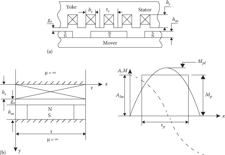
FIGURE 12.2 Single-sided F-LPMSM with iron-core primary (a) actual structure and (b) model for analysis.

μ x = [b s τ s + μ r (1 - b s τ s)] (12.2)

$μ_{x} = [\frac{b_{s}}{τ_{s}} + μ_{r} (1 - \frac{b_{s}}{τ_{s}})] (12.2)$

where

μ_r is the average magnetic permeability in the primary teeth

b_s is the slot width

τ_s is the slot pitch

A multilayer structure (Figure 12.3) is thus obtained. There are three main layers and the PM layer. The armature structure equivalent mmfs are represented by their space fundamentals distributed ac windings (q = 1, 2), placed at random heights in their layers. The regions (II + III’), containing the PMs, are isotropic (μ_x=μ_y ≈ μ₀); iron regions are infinitely permeable. The fundamentals of PM magnetization M_vPM harmonics are (in PM-secondary coordinates) as follows:

M v P M = 4 π v 2 M P M sin v 2 π \cdot τ p τ sin v 2 π τ x; M P M = H C \cdot h m; v = 1, 2 \dots (12.3)

$\begin{array}{l} M_{v P M} = \frac{4}{π v_{2}} M_{P M} \sin \frac{v_{2} π \cdot τ_{p}}{τ} \sin v_{2} \frac{π}{τ} x; & M_{P M} = H_{C} \cdot h_{m}; & v = 1, 2 \dots \end{array} (12.3)$

where

H_C is the coercive field of PMs

h_m is the PM depth

Its current sheet A_vPM = ∂M_vPM/∂x, where τ_p is the PM span/pole and τ is the pole pitch of both primary and secondary. The armature-reaction mmf fundamental and harmonics in PM-secondary coordinates would be

A v s = A v s m cos (v π x τ + γ 0) (12.4)

$A_{v s} = A_{v s m} \cos (\frac{v π x}{τ} + γ_{0}) (12.4)$

A v s m = 3 2 - \sqrt π τ k W v W 1 I v -for distributed windings (12.5)

$A_{v s m} = \frac{3 \sqrt{2}}{π τ} k_{W v} W_{1} I_{v} -for distributed windings (12.5)$

where k_Wv is the winding factor.

For tooth-wound windings, A_vsm has many large (sub and super) space harmonics around the fundamental. A full derivation of field equations with boundary conditions is presented in [1,2] for the layers I′ + I′, II, and III+III′. In Ref. [1], it was shown that the heights y_m and y_s, where the equivalent PM and armature mmfs, within the layer depth, are placed, are not important.

Images

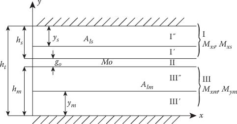
FIGURE 12.3 Multilayer model.

Finally, for the fundamental PM flux density B_yPM₁ in the airgap

E v = 2 \sqrt π ω 1 \cdot k W v \cdot τ \cdot l s t a c k \cdot (B y a v) a v; v = 1 for the fundamental (12.6)

$\begin{array}{l} E_{v} = \frac{\sqrt{2}}{π} ω_{1} \cdot k_{W_{v}} \cdot τ \cdot l_{s t a c k} \cdot {(B_{y a v})}_{a v}; & v = 1 for the fundamental \end{array} (12.6)$

(For the air-core machine, this flux density has to be calculated as an average along the air-core coil height.) The airgap inductance L_m is thus

L m v = 2 \sqrt π I k W v . τ v \cdot l s t a c k \cdot (B y a v;) v = 1 for the fundamental (12.7)

$\begin{array}{l} L_{m v} = \frac{\sqrt{2}}{π I} k_{W_{v}} . \frac{τ}{v} \cdot l_{s t a c k} \cdot (B_{y a v};) & v = 1 for the fundamental \end{array} (12.7)$

The airgap space harmonics (L_m)_v>1 are considered as leakage inductances and added to give the total synchronous cyclic inductance. For b_s/τ_s=0.53, h_s = 35 mm, τ = 114.3 mm, τ_p/τ = 0.67, μ_rel=400, g = 2 mm, h_m=6.35 mm, B_r = 0.86 T, H_C = 0.7 MA/m, and l_stack = 101.6 mm, the normal airgap flux density was calculated as mentioned earlier, measured and verified by 2D FEM for zero current and for pure I_q current (γ = π/2) as in Figure 12.4a and b [1].

Satisfactory fundamental value agreement between the analytical model and FEM is obtained while FEM fits well the Hall-probe measurements of airgap flux density. A full analytical field theory may be developed by also considering the slot openings. In addition to our isotropic slot-teeth area with μ_x ≠ μ_y, which, in fact, accounts for mmf step-like distribution due to slots and allows to use the concept of current sheet by [3]

Images

FIGURE 12.4 Airgap flux density (a) by PMs, (b) of primary mmf, (c) thrust, and (d) normal force.

B y P M v (x) = (B y P M v) s l o t l e s s \cdot P g (x); \partial B y P M v ( x , y ) \partial y + \partial B x P M v ( x , y ) \partial x = 0 (12.8)

$\begin{array}{l} B_{y P M v} (x) = {(B_{y P M v})}_{s l o t l e s s} \cdot P_{g} (x); & \frac{\partial B_{y P M v} (x, y)}{\partial y} + \frac{\partial B_{x P M v} (x, y)}{\partial x} = 0 \end{array} (12.8)$

B a v (x) = (B y v) s l o t l e s s \cdot P g (x) (12.9)

$B_{a v} (x) = {(B_{y v})}_{s l o t l e s s} \cdot P_{g} (x) (12.9)$

where P_g is the inverse per-unit airgap (or airgap) permeance function (Figure 12.5), which may be described rather precisely by conformal mapping; other simplified curve fitting is feasible.

To this scope the theory for rotary brushless dc motors [4,5] may be adopted for F-LPMSMs. In a simplified method, force at zero current F_cog may be calculated analytically by adding the forces on the primary open slot walls (Figure 12.6):

F c o g \approx l s t a c k 2 μ 0 \sum n = 1 N s \sum v = 1 \infty B 2 x P M v (v \cdot 2 π n N S + θ 1) (g α \cdot s s g) (12.10)

$F_{c o g} \approx \frac{l_{s t a c k}}{2 μ_{0}} \sum_{n = 1}^{N s} \sum_{v = 1}^{\infty} B_{x P M v}^{2} (\frac{v \cdot 2 π n}{N_{S}} + θ_{1}) (g_{α} \cdot s s g) (12.10)$

Images

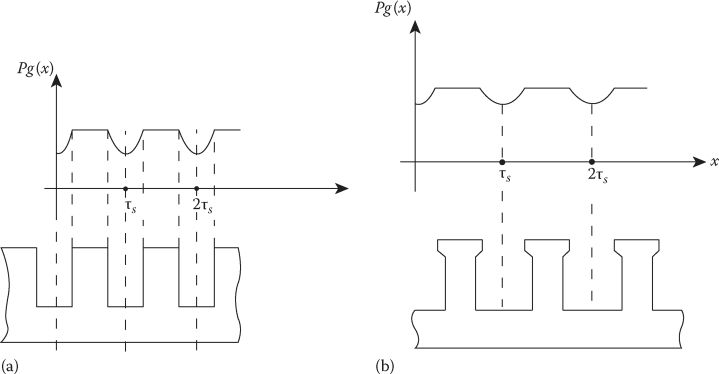
FIGURE 12.5 Inverse airgap function (a) for open slots and (b) for semiclosed slots.

Images

FIGURE 12.6 Slot flux ideal path.

where

g_α=0 and ssg=0 outside slots openings

g_α=w₁+g and ssg = 1 for left side of slots

g_α=w₂+g and ssg=-1 for the right side of slots

N_S is the number of primary slots

l_stack is the primary stack length

θ₁ is the angle of slot center with respect to PM axis

B_xPMv is obtained from (12.8)

Now the thrust may be calculated directly from the analytical field theory:

F x = l s t a c k \sum v = 1 \infty \int 0 2 p τ B y P m v (x) A s v (x) d x (12.11)

$F_{x} = l_{s t a c k} \sum_{v = 1}^{\infty} \int_{0}^{2 p τ} B_{y P m v} (x) A_{s v} (x) d x (12.11)$

F y \approx l s t a c k 2 μ 0 \sum v = 1 \infty ⎡ ⎣ ⎢ \int 0 2 p τ [B y P M v (x) + B a v (x)] 2 d x + 2 \int 0 2 p τ [(B y P M v (x) + B a v (x))] \cdot d x ⎤ ⎦ ⎥ (12.12)

$F_{y} \approx \frac{l_{s t a c k}}{2 μ_{0}} \sum_{v = 1}^{\infty} [\int_{0}^{2 p τ} {[B_{y P M v} (x) + B_{a v} (x)]}^{2} d x + 2 \int_{0}^{2 p τ} [(B_{y P M v} (x) + B_{a v} (x))] \cdot d x] (12.12)$

A comparison between calculated and measured forces (Figure 12.4c and d) shows satisfactory agreement [2]. An analytical multilayer theory may be used even for the Halbach PM array secondary (Figure 12.7) air-core F-LPMSM [6].

In this case, the PM magnetization has two components M_xn and M_zn (Figure 12.7). The PM flux linkage ψ_a per phase is [6]

Ψ P M = w n 0 p m \sum n = - \infty, o d d \infty 1 j k m γ m (j μ 0 M x n k m + μ 0 γ n M z n) \times (1 - e - γ n Δ) (e - j π n 3 - 1) (1 - e - γ n Γ) \times e - γ n x 0 e j k n x 0 (12.13)

$\begin{array}{l} Ψ_{P M} = w n_{0} p_{m} \sum_{n = - \infty, o d d}^{\infty} \frac{1}{j k_{m} γ_{m}} (\frac{j μ_{0} M_{x n}}{k_{m}} + \frac{μ_{0}}{γ_{n}} M_{z n}) \\ \times (1 - e^{- γ_{n} Δ}) (e^{- \frac{j π n}{3}} - 1) (1 - e^{- γ_{n} Γ}) \times e^{- γ_{n} x_{0}} e^{j k_{n} x_{0}} \end{array} (12.13)$

ψ a = 4 μ 0 w P s n 0 τ 3 J 0 \sum n = - \infty, o d d \infty 1 ( n π ) 4 (1 - cos π 3 n) (Γ+ e - γ n Γ - 1 γ n) (12.14)

$ψ_{a} = 4 μ_{0} w P_{s} n_{0} τ^{3} J_{0} \sum_{n = - \infty, o d d}^{\infty} \frac{1}{{(n π)}^{4}} (1 - \cos \frac{π}{3} n) (Γ+ \frac{e^{- γ_{n} Γ - 1}}{γ_{n}}) (12.14)$

E = d ψ P M d z \cdot U; U = π τ ω 1; L m = ψ a I (12.15)

$\begin{array}{l} E = \frac{d ψ_{P M}}{d z} \cdot U; & U = \frac{π}{τ} ω_{1}; & L_{m} = \frac{ψ_{a}}{I} \end{array} (12.15)$

where, say, μ₀M₀ = 1.1 T, n₀ = 1.47 × 10⁶ turns/m² (W_C = 150 turns/coil), J₀ is the current density of the coils for phase current I, k_n=2πn/2τ, where n is the mmf space harmonics order, γ_n=|k_n|, x₀=5 mm, τ = 51 mm, Γ=6 mm, Δ=25.5 mm, “stack” length w = 25.5 mm; the Halbach array contains p_m=4 + 1/2 pitches; the pole pairs of one-phase coil p_s=7. In Figure 12.7b, a good agreement between theory and experiments is proven [6].

Therefore, apparently, the analytical multilayer theory seems self-sufficient and easy to use for optimization design attempts, after preliminary design with key 2(3) D-FEM corrections.

Accounting for slot openings (and slotting in general) with magnetic saturation consideration requires the magnetic circuit method [4.7], besides 2(3) D-FEM.

Images

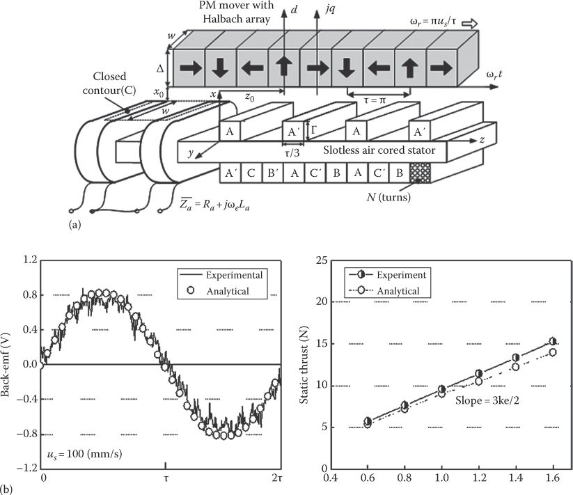
FIGURE 12.7 Air-core F-LPMSM with Halbach PM array secondary (a) emf and thrust versus iq current (b). (After Trumper, D.L. et al., IEEE Trans., IA-32(2), 371, 1996.)

12.3 Magnetic Equivalent Circuit (Mec) Theory of Iron-Core F-LPMSM

Calculating the airgap flux density distribution accounting for slot openings (in open slot magnetic cores), the actual distribution of windings in slots and magnetic saturation, within a limited computation effort means, according to the MEC method, to use realistic flux tubes and define their reluctance dependence of F-LPMSM geometry, mover position, and magnetic saturation, slot by slot and tooth by tooth (Figure 12.8), all assembled in a complete MEC (magnetostatic) model, to be solved by algebraic methods. In a flux tube, the flux density is considered uniform; this idea leads to the level of complexity (number of flux tubes—reluctances of MEC).

The structure of the MEC has to be fixed during motion, to secure limited computation effort. A two PM pole structure with its primary section of MEC is shown in Figure 12.8 [7].

A bi-section for airgap and yet another one for the PM secondary are added [7]. Also visible in Figure 12.8b are the longitudinal leakage reluctances R_gz, “attached” to primary (to the middle of the airgap); they are constant; only the tooth reluctance R_t varies due to magnetic saturation. The other side of airgap MEC (Figure 12.9) contains the reluctances R_mg₁, R_mg₂, and R_mg₃, which vary with primary position (motion). The MEC of the 2-pole secondary (Figure 12.9b) is rather straightforward.

Images

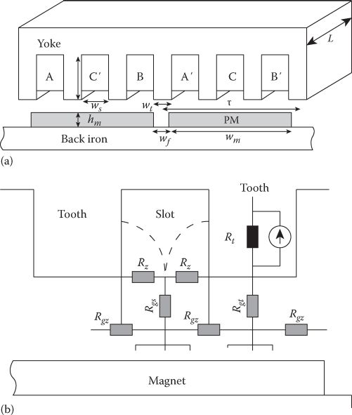
FIGURE 12.8 Iron-core F-LPMSM geometry (a) and elementary MEC, (b). (After Sheikh-Ghalavand, B. et al., IEEE Trans, MAG-46(1), 112, 2010.)

Images

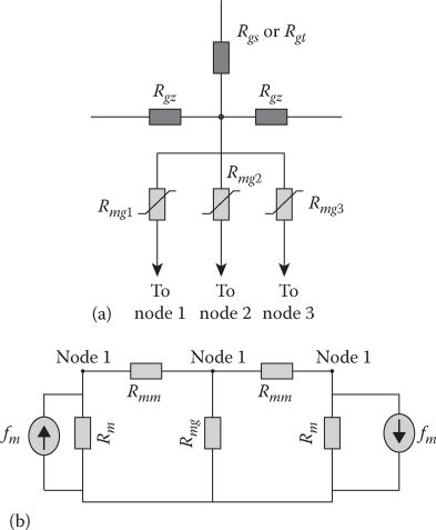
FIGURE 12.9 Airgap secondary MEC (a) and PM-secondary MEC (b). (After Sheikh-Ghalavand, B. et al., IEEE Trans,, MAG-46(1), 112, 2010.)

The magnetic reluctances of the entire MEC are defined by using Ampere’s law. Finally, the complete MEC of the 2 PM pole secondary iron-core F-LPMSM is shown in Figure 12.10 [7].

A typical result, related to flux density in the middle of the teeth in saturated conditions and shown in Figure 12.11, indicates quite good agreement with FEM. This good agreement is valid also for thrust, and it may be used to develop a reliable iron-core loss model, by assuming a linear variation in time of flux density in primary teeth and yoke as in Figure 12.12.

Images

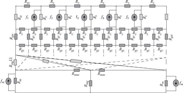
FIGURE 12.10 Complete MEC model of 2-pole PM-secondary F-LPMSM. (After Sheikh-Ghalavand, B. et al., IEEE Trans, MAG-46(1), 112, 2010.)

Images

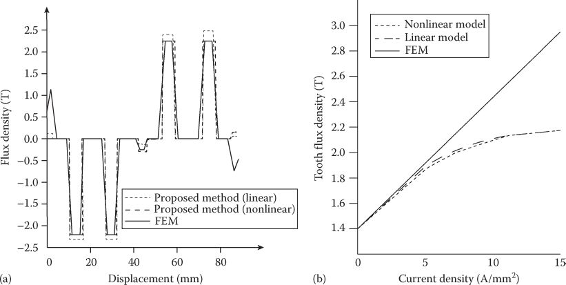
FIGURE 12.11 Flux density in the middle of the teeth (a) and flux density in tooth 2 versus primary current density, (b). (After Sheikh-Ghalavand, B. et al., IEEE Trans, MAG-46(1), 112, 2010.)

Traditionally, the primary core losses are separated into two terms: the hysteresis losses p_h and eddy current losses p_eddy.

p i r o n = p h + p e d d y = k h \cdot B α max (f 1 50) + k e \cdot B 2 max (f 1 50) 2 W/m 3 (12.16)

$p_{i r o n} = p_{h} + p_{e d d y} = k_{h} \cdot B_{\max}^{α} (\frac{f_{1}}{50}) + k_{e} \cdot B_{\max}^{2} {(\frac{f_{1}}{50})}^{2} {W/m}^{3} (12.16)$

where

α=1.8-2.2

k_h and k_e are core losses per m³ of laminated core at 1 T and 50 Hz

As (12.16) is valid for sinusoidal flux density-time variation, it gives large errors for waveforms as in Figure 12.12 and thus

p e d d y = 2 k e T \int 0 T (d B ( t ) d t) 2 d t (W/m 3) (12.17)

$p_{e d d y} = \frac{2 k_{e}}{T} \int_{0}^{T} {(\frac{d B (t)}{d t})}^{2} d t ({W/m}^{3}) (12.17)$

B_t_max and B_y_max are calculated by the MEC method or by FEM. The total eddy current losses for the waveforms in Figure 12.12 are

p e \approx 12 q 1 k e k c l (U τ B t max) 2 V t e e t h + 8 q 1 k e k c l τ W m (U τ B y max) 2 V y o k e (W) (12.18)

$p_{e} \approx 12 q_{1} k_{e} k_{c l} {(\frac{U}{τ} B_{t \max})}^{2} V_{t e e t h} + 8 q_{1} k_{e} k_{c l} \frac{τ}{W_{m}} {(\frac{U}{τ} B_{y \max})}^{2} V_{y o k e} (W) (12.18)$

with

W_m is the PM span per pole

k_d = 1.1−1.2 accounts for longitudinal eddy currents in the core

q₁ is slots/pole/phase

The PM-secondary losses, due to slot openings and primary mmf space harmonics fields, have not been considered here. Results from FEM and MEC indicate a total relative error below 5% in total primary core losses [7].

Note: The tooth-wound primary exhibits a rich content of mmf space harmonics, but the MEC method can also be used for it. Finally, the current-time particular variations end up in flux density—time variations, and sufficiently small time periods may handle the situation. Ultimately, perhaps, only FEM can produce reliable enough results for total core losses during steady state and transients, accounting for both space harmonics and time harmonics.

Images

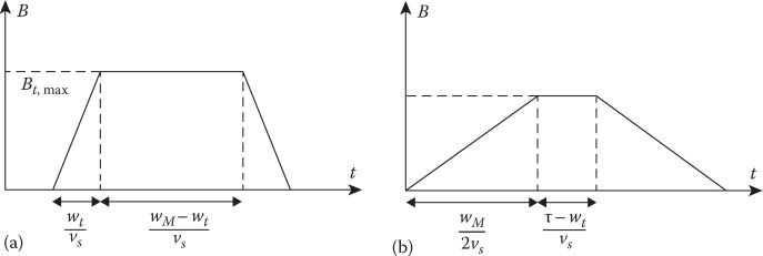
FIGURE 12.12 Ideal (linear) time variation of flux density in primary teeth (a) and yoke (b). (After Sheikh-Ghalavand, B. et al., IEEE Trans., MAG-46(1), 112, 2010.)

12.4 Analytical Multilayer Field Theory of Air-Core F-LPMSM

The multilayer field theory of air-core F-LPMSM (Figure 12.13a) may be approached with the same method as in Section 12.2, with the simplification that the slot zone is the ac coils zone and μ=μ₀. To add more generality to the model, the case of rectangular current control is considered (Figure 12.13b) [8].

The PM magnetization M(x) is decomposed in Fourier series:

M (x) = 4 π B r μ 0 \sum v = 1 \infty 1 2 v - 1 sin (2 v - 1) π 2 τ p τ sin (2 v - 1) π τ h m \times \times exp [- (2 v - 1) π τ y] sin (2 v - 1) π τ x (12.19)

$\begin{array}{l} M (x) = \frac{4}{π} \frac{B_{r}}{μ_{0}} \sum_{v = 1}^{\infty} \frac{1}{2 v - 1} \sin (2 v - 1) \frac{π}{2} \frac{τ_{p}}{τ} \sin (2 v - 1) \frac{π}{τ} h_{m} \times \\ \times \exp [- (2 v - 1) \frac{π}{τ} y] \sin (2 v - 1) \frac{π}{τ} x \end{array} (12.19)$

The final B_xI, B_yI, PM flux density components in region I [8], are

B x l (x, y) = 4 B r π \sum v = 1 \infty 1 2 v - 1 sin (2 v - 1) π 2 τ p τ sinh (2 v - 1) π τ h m \times exp (- (2 v - 1) π τ y) \cdot sin (2 v - 1) π τ x B x l (x, y) = 4 B r π \sum v = 1 \infty 1 2 v - 1 sin (2 v - 1) π 2 τ p τ sinh (2 v - 1) π τ h m \times exp (- (2 v - 1) π τ y) \cdot cos (2 v - 1) π τ x (12.20)

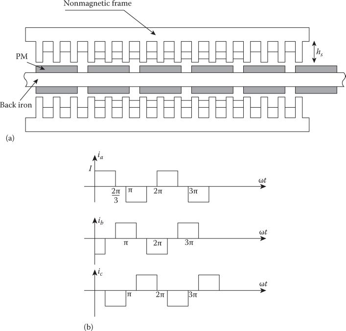
$\begin{array}{l} B_{x l} (x, y) = \frac{4 B_{r}}{π} \sum_{v = 1}^{\infty} \frac{1}{2 v - 1} \sin (2 v - 1) \frac{π}{2} \frac{τ_{p}}{τ} \sinh (2 v - 1) \frac{π}{τ} h_{m} \times \exp (- (2 v - 1) \frac{π}{τ} y) \cdot \sin (2 v - 1) \frac{π}{τ} x \\ B_{x l} (x, y) = \frac{4 B_{r}}{π} \sum_{v = 1}^{\infty} \frac{1}{2 v - 1} \sin (2 v - 1) \frac{π}{2} \frac{τ_{p}}{τ} \sinh (2 v - 1) \frac{π}{τ} h_{m} \times \exp (- (2 v - 1) \frac{π}{τ} y) \cdot \cos (2 v - 1) \frac{π}{τ} x \end{array} (12.20)$

Images

FIGURE 12.13 Double-sided air-core F-LPMSM, (a) and its ideal (rectangular) phase currents, (b).

B_xI and B_yI are dependent on B_r, τ_P/τ, h_m/τ, and they decay along Oy (airgap and winding depth). The fundamental components decay e times along τ/π airgap depth. To secure a good interaction between PM field and the primary air-core winding, the latter’s depth h_s should be smaller than τ/π; so larger pole pitch allows deeper windings. In a rectangular, current-controlled F-LPMSM, the two active phase mmf angle shifts with respect to PM flux density axis from 60° to 120° electrical degrees (Figure 12.14).

Using the Lorenz force formula, the thrust F_x and normal force F_y force (on primary side) are

F x (t) = 64 \cdot n c I \cdot l s t a c k w s \sum v = 1 \infty C v cos (2 v - 1) π 6 [cos (2 v - 1) (π τ U \cdot t - π 6)] F x (t) = 64 \cdot n c I \cdot l s t a c k w s \sum v = 1 \infty C v sin (2 v - 1) π 6 [cos (2 v - 1) (π τ U \cdot t - π 6)] (12.21)

$\begin{array}{l} F_{x} (t) = \frac{64 \cdot n_{c} I \cdot l_{s t a c k}}{w_{s}} \sum_{v = 1}^{\infty} C_{v} \cos (2 v - 1) \frac{π}{6} [\cos (2 v - 1) (\frac{π}{τ} U \cdot t - \frac{π}{6})] \\ F_{x} (t) = \frac{64 \cdot n_{c} I \cdot l_{s t a c k}}{w_{s}} \sum_{v = 1}^{\infty} C_{v} \sin (2 v - 1) \frac{π}{6} [\cos (2 v - 1) (\frac{π}{τ} U \cdot t - \frac{π}{6})] \end{array} (12.21)$

Images

FIGURE 12.14 Primary mmf angle PM axis; from 60° to 120° for rectangular current control (a) and F_x, F_y forces (b) for the data in Table 12.1.

TABLE 12.1
Air-Core F-LPMSM Data

Images

with

C υ = 4 B r τ 2 π 3 h s ( 2 v - 1 ) 3 sin (2 v - 1) π 2 τ p τ sinh (2 v - 1) π 2 h m exp [- (2 v - 1) π τ h m] \times [1 - exp (- (2 v - 1) (h s + g) π τ) sin (2 v - 1) π h s 2 g] (12.22)

$\begin{array}{l} C_{υ} = \frac{4 B_{r} τ^{2}}{π^{3} h_{s} {(2 v - 1)}^{3}} \sin (2 v - 1) \frac{π}{2} \frac{τ_{p}}{τ} \sinh (2 v - 1) \frac{π}{2} h_{m} \exp [- (2 v - 1) \frac{π}{τ} h_{m}] \\ \times [1 - \exp (- (2 v - 1) (h_{s} + g) \frac{π}{τ}) \sin (2 v - 1) \frac{π h_{s}}{2 g}] \end{array} (12.22)$

In (12.21) and (12.22), l_stack is the “stack” or active depth of primary and secondary (PM). Plots of forces in Figure 12.14 correspond to the data in Table 12.1, over a 60° electrical degree interval, when phases A + B are active and show notable variations. F_x variations are important and they may be further reduced by varying PM span ratio τ_p/τ, h_S/τ, g/τ, or even the PM shape and W_S/τ_S ratio. The total normal force on the PM secondary is practically zero, or small, for zero eccentricity. (F_y in Figure 12.14 is related to one primary side.)

The 3D aspect of the field is not considered but it could be added, by an additional decomposition in Fourier series along z (l_stack) direction. A 3D-FEM would yield even better results but for a much larger computation effort. The emfs for the three phases e_a,b,c are

e a, b, c = \sum C n U cos (π τ U t + γ 0 - (i - 1) 2 π 3); i = 1, 2, 3 (12.23)

$\begin{array}{l} e_{a, b, c} = \sum C_{n} U \cos (\frac{π}{τ} U t + γ_{0} - (i - 1) \frac{2 π}{3}); & i = 1, 2, 3 \end{array} (12.23)$

So the thrust may also be written as

F x = 1 U (e a i a + e b i b + e c i c) (12.24)

$F_{x} = \frac{1}{U} (e_{a} i_{a} + e_{b} i_{b} + e_{c} i_{c}) (12.24)$

For q = 1 (3 slots/pole), the phase self and mutual inductances L_aa and L_ab may be approximated as [9]

L a a = L s l + μ 0 W 2 1 τ \cdot l s t a c k ( 1 + k f r i n g e ) p ( g + h m ) (12.25)

$L_{a a} = L_{s l} + \frac{μ_{0} W_{1}^{2} τ \cdot l_{s t a c k} (1 + k_{f r i n g e})}{p (g + h_{m})} (12.25)$

L a b = - L a a - L s l 3; L s l - leakage inductance (12.26)

$\begin{array}{l} L_{a b} = - \frac{L_{a a} - L_{s l}}{3}; & L_{s l} - leakage inductance \end{array} (12.26)$

The fringing coefficient k_fringe > 0 accounts for longitudinal flux density and transverse (3D) field components; k_fringe may be calculated from the multilayer theory (in 3D form), from 3D-FEM or from current decay measurements at standstill.

Before approaching the circuit model of F-LPMSMs, required for performance evaluation and for dynamics and control design, let us first focus a little on the cogging force and its particular end effect in F-LPMSMs.

12.5 Cogging Force and Longitudinal End Effects

The cogging (zero current), or detent, force is the result of the variation of the coenergy stored in the PMs due to the iron-core slot openings. It is a periodic function that, for rotary PMSMs, has the period of LCM (N_s, 2p), where N_s is the number of rotor poles:

LCM (N s, 2 p) = N s GCD ( N s , 2 p ) (12.27)

$LCM (N_{s}, 2 p) = \frac{N_{s}}{GCD (N_{s}, 2 p)} (12.27)$

GCD is the largest common divisor.

For L-PMSM, 2pτ in the secondary should be considered to correspond to N_Sτ_s in the primary (τ_s is the slot pitch). For tooth-wound windings, LCM becomes larger than for distributed windings (even with q₁ = 1 slot/pole/phase) and, consequently, the cogging force gets smaller.

Two tooth-wound F-LPMSMs situations, which correspond to 9 slots/12 poles and 10 slots/9 poles, are shown in Figure 12.15.

The configuration with 10 slots and 9 poles is somewhat unusual as it still hosts 3 × 3 phase coils, but it is used purposely to drastically reduce the cogging force. As LCM (9, 12) is 36 and LCM (9, 10) is 90, a high number of cogging force periods is expected. With the latter solution and in the form of 10 slots and 9 PM poles per module length, the periodicity of cogging force is even higher (in the ratio of 10/3 and not 10/4) [10]:

F 9 / 12 (x) = 9 \sum A 3 n sin (3 n π τ x + α 3 n) F 10 / 9 (x) = 10 \sum A 10 n sin (10 n π τ x + α 10 n) (12.28)

$\begin{array}{l} F_{9 / 12} (x) = 9 \sum A_{3 n} \sin (3 n \frac{π}{τ} x + α_{3 n}) \\ F_{10 / 9} (x) = 10 \sum A_{10 n} \sin (10 n \frac{π}{τ} x + α_{10 n}) \end{array} (12.28)$

The results in Figure 12.16 show that even if the peak cogging force of each slot is about the same in both cases, their phase shift is such that the total cogging force for the 10 slot/9 pole F-LPMSM is almost zero [10]. Even a single slot cogging force, if uncompensated, can lead to a large cogging force. This may be called the end effect in cogging force. A typical 9 slot/8 pole combination would show it.

Images

FIGURE 12.15 Two tooth-wound F-LPMSMs: (a) 9/12. (b) 10/9. (After Baatar, N. et al., IEEE Trans., MAG-45(10), 4562, 2009.)

Images

FIGURE 12.16 Cogging force: (a) for 9 slots/12 poles, (b) for 10 slots/9 poles. (After Baatar, N. et al., IEEE Trans, MAG-45(10), 4562, 2009.)

Apart from slot pitch PM to pole pitch ratio, primary shape optimization may be used to reduce the drag force due to primary (or PM secondary) finite length, especially in short-length modules. Chamfering and widening the end tooth is a way to do it (Figure 12.17)

The question is if these methods that reduce the cogging (and drag) force will not impede on average total thrust; not so for the aforementioned configuration (10 slots/9 poles) and chamfered end teeth of primary [10]. Now that the principle of cogging force occurrence is elucidated, let us remember that all methods to reduce cogging torque in rotary PMSMs may be applied for LPMSMs, to reduce the cogging force. Among them we enumerate here

Optimization of PM span τ_p per pole pitch τ [11]
Pole displacement (in pairs), slot opening optimization
Making a PM pole of a few sectors as in PWM signals [12] with notable average thrust reduction
Simple (or double) skewing [13], with notable average thrust reduction
PM shaping (bread loaf shape) for sinusoidal emf
Double sided topology for zero normal force [14]
Current waveform shaping

Images

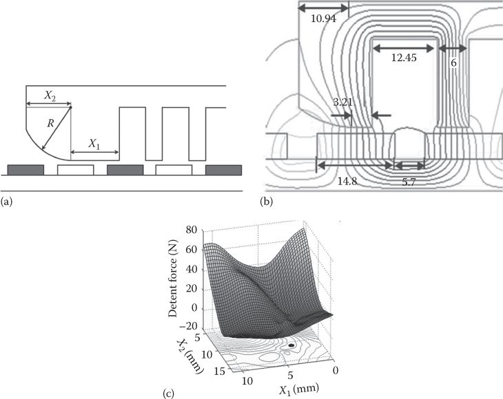
FIGURE 12.17 Drag force due to finite primary length at zero current: (a) variables X1, X2, (b) final geometry, and (c) drag force. (After Baatar, N. et al., IEEE Trans., MAG-45(10), 4562, 2009.)

12.5.1 End Effects in 2(4) Pole PM-Secondary F-LPMSMs

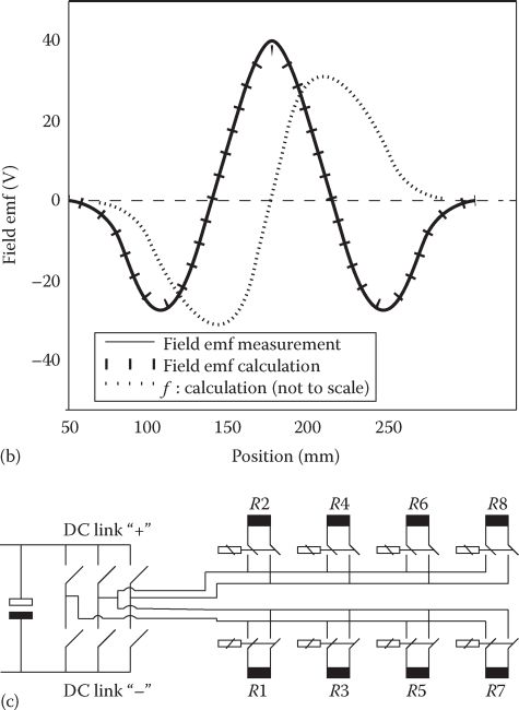
In some applications where, say, short length PM movers are required, a 2-pole short PM secondary may be adopted while the long primary is the stator, supplied in sections to keep the copper losses low. In such a configuration (Figure 12.18), with air-core windings, two phase (rather than three-phase) ac windings are used (to avoid nonbalanced phase current due to non-equal self and mutual inductances) [15]. The PM flux per one stator coil versus mover position (Figure 12.18b) shows that the emf in the coil has one full-scale positive and two half-scale negative peak values. To smooth the total thrust, two coils in series have to be connected for the negative polarity of emf, according to mover position [15]. This change in coil connection needs a special power electronics system, to feed the long stator sequentially (Figure 12.18).

The usage of 2(4) pole PM mover is to be avoided whenever possible as it creates problems in the switching of the active stator windings section after section. In any case, 3D-FEM is to be used to analyze such topologies with air core (or with iron core).

Images

FIGURE 12.18 Two-pole PM mover air-core F-LPMSM (a). The emf coil vs. mover position, (b) converter plus coil switches for one stator phase (there are two phases in all) (c). (After Henneberger, G. and Reuber, C., A linear synchronous motor for a clean room system, Record of LDIA-1995, Nagasaki, Japan, pp. 227–230, 1995.)

Images

12.6 dq Model of F-LPMSM With Sinusoidal EMF

As seen earlier in this chapter, proper design may lead to rather sinusoidal emfs in the 3(2) phases of primary of F-LPMSMs. If we further treat the cogging force (the force at zero current) as a disturbance (load) force, then we may apply safely the dq model; for tooth-wound primaries, this model reflects the action of mmf fundamental as for distributed-winding primaries.

Thrust pulsations due to space harmonics consequences in emf or mmf are not considered in the standard dq model of electric machinery. Despite the approximation, the dq model is widely used to assess basic steady-state and dynamic performance of F-LPMSMs. The dq model also provides the ideal tool for the design of position, speed, or thrust (and normal force, eventually) control via FOC or DTFC.

So far we inferred that only surface PM secondaries are practical for F-LPMSM, but, for the sake of generality, different d−q inductances L_d and L_q are considered in the dq model. This is the case in mixed (PM + dc controlled coils) excitation secondary with long active stator MAGLEVs with buried PMs on mover, to leave room for the addition of slots to host an ac two-phase generator on board the mover, based on stator mmf space harmonics field (q₁ = 1), Figure 12.19 (L_d < L_q). The role of PMs in Figure 12.19b is quite different [16]: they are placed along axis q in multiple flux barriers and the dc coils in axis d (L_d > L_q). The PMs serve for wide constant power speed range and for operation at unity power factor (minimum converter kVA).

Images

FIGURE 12.19 PM-hybrid secondary (mover) and active stator F-LPMSM (a) with PM + dc coils in axis d and (b) dual-axis-field linear BEGA. (After Boldea, I. and Tutelea, L., Electric Machines: Steady State, Transients and Design with Matlab, CRC Press, Taylor & Francis, New York, 2009.)

To a first approximation, the magnetization inductances L_md and L_mq in Figure 12.19 are (as for its rotary machine counterparts) [17] as follows:

L d m = L m \cdot k d m 1 + k s d; L q m = L m \cdot k q m 1 + k s q (12.29)

$\begin{array}{l} L_{d m} = L_{m} \cdot \frac{k_{d m}}{1 + k_{s d}}; & L_{q m} = L_{m} \cdot \frac{k_{q m}}{1 + k_{s q}} \end{array} (12.29)$

k d m = (τ p τ + 1 π sin τ p τ π) \cdot g g + h P M τ 2 l P M (12.30)

$k_{d m} = (\frac{τ_{p}}{τ} + \frac{1}{π} \sin \frac{τ_{p}}{τ} π) \cdot \frac{g}{g + h_{P M} \frac{τ}{2 l_{P M}}} (12.30)$

k d m = τ p τ - 1 π sin τ p τ π + 2 3 π cos τ p τ π 2 (12.31)

$k_{d m} = \frac{τ_{p}}{τ} - \frac{1}{π} \sin \frac{τ_{p}}{τ} π+ \frac{2}{3 π} \cos \frac{τ_{p}}{τ} \frac{π}{2} (12.31)$

L m = 6 μ 0 ( k W 1 W 1 p ) τ \cdot l s t a c k π 2 p \cdot g \cdot k C (12.32)

$L_{m} = \frac{6 μ_{0} (k_{W_{1}} W_{1 p}) τ \cdot l_{s t a c k}}{π^{2} p \cdot g \cdot k_{C}} (12.32)$

For a long stator, L_md and L_mq refer only to the stator part covered by the PM-hybrid secondary. For the rest of “open” stator, the inductance, treated as a leakage inductance L_p’₋_p, is

L p' - p \approx L t p' - p + 6 μ 0 ( k W 1 W 1 p ' ) 2 τ \cdot l s t a c k π 2 ( p ' - p ) τ π L d = L d m + L l p + L p' - p; L q = L q m + L l p + L p' - p (12.33)

$\begin{array}{l} L_{p^{'} - p} \approx L_{t p^{'} - p} + \frac{6 μ_{0} {(k_{W_{1}} W_{1 p^{'}})}^{2} τ \cdot l_{s t a c k}}{π^{2} (p^{'} - p) \frac{τ}{π}} \\ \begin{array}{l} L_{d} = L_{d m} + L_{l p} + L_{p^{'} - p}; & L_{q} = L_{q m} + L_{l p} + L_{p^{'} - p} \end{array} \end{array} (12.33)$

The total number of pole pairs per energized section is p′ (p -c p’) out of which p of them correspond to active part (in interaction with the mover); the airgap of the open stator part of section is considered τ/π as it would result from a 2D analytical field solution. For linear BEGA [16], the expressions of parameters are similar to those of rotary PM assisted reluctance synchronous motors.

For a short primary, L_d and L_q would be simply (for 2p-poles)

L d = L l s + L d m; L q = L l s + L q m; L l s - leakage inductance (12.34)

$\begin{array}{l} L_{d} = L_{l s} + L_{d m}; & L_{q} = L_{l s} + L_{q m}; & L_{l s} - leakage inductance \end{array} (12.34)$

The resistance/phase formula will be given in the forthcoming design paragraph. So, in PM-secondary dq coordinates, Figure 12.19, the dq model of F-LPMSMs writes

V ¯ ¯ ¯ S = R S I ¯ S + d ψ ¯ ¯ S d t + j π τ U k \cdot ψ ¯ ¯ S; ψ ¯ ¯ S = L d I d + ψ P M + j L q I q (12.35)

$\begin{array}{l} {\bar{V}}_{S} = R_{S} {\bar{I}}_{S} + \frac{d {\bar{ψ}}_{S}}{d t} + j \frac{π}{τ} U k \cdot {\bar{ψ}}_{S}; & {\bar{ψ}}_{S} = L_{d} I_{d} + ψ_{P M} + j L_{q} I_{q} \end{array} (12.35)$

V ¯ ¯ ¯ S = V d + j V q; I ¯ S = I d + j I q; F x = 3 2 π τ [ψ P M d + (L d - L q) I d] (I q k) (12.36)

$\begin{array}{l} {\bar{V}}_{S} = V_{d} + j V_{q}; & {\bar{I}}_{S} = I_{d} + j I_{q}; & F_{x} = \frac{3}{2} \frac{π}{τ} [ψ_{P M d} + (L_{d} - L_{q}) I_{d}] (I_{q k}) \end{array} (12.36)$

k = 1 for PM-secondary mover and k=−1 for primary mover.

The motion equations are

G v d U d t = F x - F l o a d - F c o g g (x); d x d t = U (12.37)

$\begin{array}{l} G_{v} \frac{d U}{d t} = F_{x} - F_{l o a d} - F_{c o g g} (x); & \frac{d x}{d t} = U \end{array} (12.37)$

G m d U g d t = F n - G m \cdot g - F d i s; d g d t = U g; γ = tan - 1 (I d I q) (12.38)

$\begin{array}{l} G_{m} \frac{d U_{g}}{d t} = F_{n} - G_{m} \cdot g - F_{d i s}; & \frac{d g}{d t} = U_{g}; & γ = {tan}^{- 1} (\frac{I_{d}}{I_{q}}) \end{array} (12.38)$

F \approx ( B 2 P M g + B 2 a g + 2 B P M g \cdot B a g \cdot sin γ ) 2 μ 0 2 p \cdot τ \cdot l s t a c k 2 (12.39)

$F \approx \frac{(B_{P M g}^{2} + B_{a g}^{2} + 2 B_{P M g} \cdot B_{a g} \cdot \sin γ)}{2 μ_{0}} \frac{2 p \cdot τ \cdot l_{s t a c k}}{2} (12.39)$

Bp_M, B_ag are PM and armature airgap flux density fundamentals.

U_g is the vertical speed in case the airgap varies (due to track irregularities or during levitation control). The Park transformation completes the system:

∣ ∣ ∣ ∣ ∣ V d V q V 0 ∣ ∣ ∣ ∣ ∣ = 2 3 ∣ ∣ ∣ ∣ ∣ cos (- π τ x) cos (- π τ x + 2 π 3) cos (- π τ x - 2 π 3) sin (- π τ x) sin (- π τ x + 2 π 3) sin (- π τ x - 2 π 3) 1 2 1 2 1 2 ∣ ∣ ∣ ∣ ∣ ∣ ∣ ∣ ∣ V a V b V c ∣ ∣ ∣ ∣ (12.40)

$| \begin{array}{l} V_{d} \\ V_{q} \\ V_{0} \end{array} | = \frac{2}{3} | \begin{array}{l} \begin{array}{l} \cos (- \frac{π}{τ} x) & \cos (- \frac{π}{τ} x + \frac{2 π}{3}) & \cos (- \frac{π}{τ} x - \frac{2 π}{3}) \end{array} \\ \begin{array}{l} \sin (- \frac{π}{τ} x) & \sin (- \frac{π}{τ} x + \frac{2 π}{3}) & \sin (- \frac{π}{τ} x - \frac{2 π}{3}) \end{array} \\ \begin{array}{l} \frac{1}{2} & \frac{1}{2} & \frac{1}{2} \end{array} \end{array} | | \begin{array}{l} V_{a} \\ V_{b} \\ V_{c} \end{array} | (12.40)$

Given the phase voltages V_a(t), V_b(t), V_c(t), the initial values of variables (I_d₀, I_q₀, U₀, X₀, U_g₀, g₀) and force perturbations (F_cogg(x) and F_dis(x)), and the load force F_load, together with machine parameters values, the dq model equations may be solved numerically for any steady-state or transient operation mode, with constant or variable airgap g. However, for propulsion control purposes, a few typical control law steady-state characteristics are worthy of discussion. Before that, the equivalent circuits for transients and the structural diagram are given for completeness. Adding the primary and secondary core loss via equivalent resistances (R_pcore, R_score), the dq model equations at constant speed, U = const., and constant airgap, g = const., yield the equivalent circuits in Figure 12.20. They are similar to those of rotary IPMSMs. The structural diagram in Figure 12.21 is valid for propulsion only (constant airgap).

The space phasor diagrams for motoring and generating are similar to those of rotary PMSMs [17].

Images

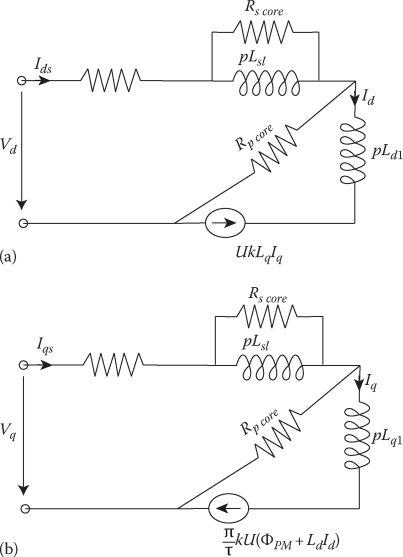
FIGURE 12.20 Equivalent circuits: (a) axis d and (b) axis q.

Images

FIGURE 12.21 F-LPMSM structural diagram for propulsion only.

12.7 Steady-State Characteristics for Typical Control Strategies

There are quite a few control strategies of practical interest for F-LPMSMs. We select here two ol them:

Maximum thrust/current control
Flux weakening control

12.7.1 Maximum Thrust per Current Characteristics (L_d = L_q = L_s)

Core losses are neglected for simplicity:

So, from (12.33) and (12.34), for surface PM-secondary (L_d=L_q=L_s),

F x = 3 2 π τ ψ P M d I q (12.41)

$F_{x} = \frac{3}{2} \frac{π}{τ} ψ_{P M d} I_{q} (12.41)$

Zero I_d is thus automatically maximum thrust/current. Consequently,

V 2 s = (2 L s U F x 3 ψ P M d) 2 + (2 R s F x 3 π ψ P M d + π τ U ψ P M d) 2 (12.42)

$V_{s}^{2} = {(\frac{2 L_{s} U F_{x}}{3 ψ_{P M d}})}^{2} + {(\frac{2 R_{s} F_{x}}{3 {πψ}_{P M d}} + \frac{π}{τ} U ψ_{P M d})}^{2} (12.42)$

This is a typically mild mechanical characteristic: (thrust/speed curve), but with a definite ideal no load speed U_i₀ (Figure 12.22).

$\begin{array}{l} {(U_{i 0})}_{I_{q} = I_{s} = 0} = \frac{V_{s} τ}{{πψ}_{P M d}}; & V_{S} = V \sqrt{2}; & V : phase voltage (RMS) \end{array} (12.43)$

The normal force (γ=0) is (12.39)

$F_{n} = \frac{(B_{P M q_{1}}^{2} + B_{a g}^{2}) p τ l_{s t a c k}}{2 μ_{0}} (12.44)$

but

$B_{P M q_{1}} = \frac{π}{2} \frac{ψ_{P M d}}{l_{s t a c k} τ W_{1} k_{W_{1}}} (12.45)$

and

${(B_{a g 1})}_{I d = 0} = \frac{L_{q m} I_{s}}{\frac{π}{2} l_{s t a c k} τ W_{1} k_{W_{1}}} (12.46)$

Images

FIGURE 12.22 Constant (I_d = 0) speed/thrust curves (f = u/2τ, variable).

$F_{n} = {(\frac{π}{2} \frac{1}{l_{s t a c k} τ W_{1} k_{W_{1}}})}^{2} ψ_{P M d}^{2} [1 + {(\frac{L_{q m} I_{s}}{ψ_{P M d}})}^{2}] \frac{p τ l_{s t a c k}}{2 μ_{0}} (12.47)$

Consequently, the normal force increases with load (I_S = jI_q, that is, with F_x). This may lead to increased noise and vibration in the mover.

12.7.2 Maximum Thrust/Flux (L_d = L_q = L_s)

Flux weakening is today attempted with surface PM secondary for tooth-wound primary whose total inductance L_s is rather large (due to added large differential leakage inductance of primary mmf space harmonics). A large L_s means a not so large demagnetizing current I_d < 0. For constant ψ_S

$\begin{array}{l} ψ_{S}^{2} = {(ψ_{P M d} + L_{s} I_{s})}^{2} + L_{s}^{2} I_{q}^{2}; & F_{x} = \frac{3}{2} \frac{π}{τ} ψ_{P M d} I_{q} \end{array} (12.48)$

with I_q from F_x in the flux ψ_S:

${(\frac{V_{s}}{\frac{π}{τ} U})}^{2} = ψ_{S}^{2} = {(ψ_{P M d} + L_{s} I_{d})}^{2} + L_{s}^{2} {(\frac{3}{2} \frac{π}{τ} ψ_{P M d})}^{- 2} F_{x}^{2} (12.49)$

The maximum thrust F_x per given ψ_S (or given speed U and voltage V_S) in (12.48):

$ψ_{P M d} + L_{s} I_{d k} = 0 (12.50)$

$I_{d k} = - \frac{ψ_{P M d}}{L_{s}} (12.51)$

However, in such conditions for F_x=0 (ideal no load) in (12.49), U₀ = ∞ (infinite ideal no load speed). The force/speed curve for different values of I_d ≠ 0 are shown in Figure 12.23 for given voltage V_S = V_S _max.

This time the thrust and normal force from (12.39) and (12.44) through (12.48) are

$\begin{array}{l} F_{x} \frac{3}{2} \frac{π}{τ} ψ_{P M d} I_{s} \cos γ; & for F_{x} < γ > 90 \end{array} ° (12.52)$

Images

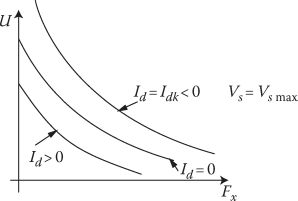
FIGURE 12.23 Speed/thrust curve for nonzero I_d.

$\begin{array}{l} F_{n} = {(\frac{π}{2} \frac{1}{l_{s t a c k} τ W_{1} k_{W_{1}}})}^{2} ψ_{P M d}^{2} [1 + {(\frac{L_{q m} I_{s}}{ψ_{P M d}})}^{2} + 2 \frac{L_{q m} I_{s}}{ψ_{P M d}} \sin γ] \cdot \frac{p τ l_{s t a c k}}{2 μ_{0}} \\ \begin{array}{l} γ = {tan}^{- 1} (\frac{I_{d}}{I_{q}}); & γ < 0 & for I_{d} < 0 \end{array} \end{array} (12.53)$

$\begin{array}{l} I_{s} = \sqrt{I_{d}^{2} + I_{q}^{2}}; & L_{q m} = L_{m} & L_{d} = L_{q} \end{array} (12.54)$

The normal force may be controlled by the angle γ ≠ 0, and the thrust may be varied by the current amplitude, I_s. F_x and F_n both depend on γ and I_s, so their control is not decoupled. This has consequences when integrated propulsion and levitation are targeted.

Note: For L_d ≠L_q, the maximum thrust/flux conditions yield a different ${I^{'}}_{d k} \neq I_{d k} = - ψ_{P M s} / L_{s}$ (see Ref. [18], for more details).

Example 12.1

F-LPMSM with L_d=L_q = L_S characteristics

Let us consider a flat F-LPMSM with a surface PM secondary and the following data:

V_s_max = 120 V (RMS) per phase, T = 0.06 m, B_gM1 = 0.7 T, L_d = L_q = L_s = 30 mH, R_S=3 Ω, stack length lstack=0.1 m, 2p = 4 poles, q = 1 slot/pole/phase single layer winding, and W₁ = 400 turns/phase.

Calculate:

The PM flux linkage per phase ψ_PM_d.
For I_d=0 the ideal no load speed U_i₀ and the corresponding (maximum) frequency ω_1max.
For U_S = U_i₀/2 and I_q₀ = −10 A (I_d=0), determine the thrust F_x and the voltage, frequency, thrust/watt losses (N/W), and specific thrust (N/cm²).
For same U_S = U_i₀/2 and I_d = I_dk/3 = -ψ_PMd/3L_S calculate I_q, thrust, and voltage, and discuss the results; calculate the efficiency and power factor.
What current density is needed in the winding design; are the data realistic?

Solution

The PM flux linkage per phase ψ_PMd is

$ψ_{P M d} \approx \frac{2}{π} B_{P M g 1} τ \cdot I_{s t a c k} \cdot W_{1} k_{W_{1}} = \frac{2}{π} \times 0.7 \times 0.06 \times 0.1 \times 800 \times 1 \times = 1.07 W b (12.55)$
(b) The ideal no load speed U,₀ is

$U_{i 0} = \frac{V_{s} \cdot τ}{π \cdot ψ_{P M d}} = \frac{120 \sqrt{2} \times 0.06}{π \times 1 .07} = 3.02 \times \frac{π}{0.06} = 158.0 rad/s (12.56)$

So

$f_{lm ax} = \frac{ω_{lm ax}}{2 π} = 25 H z$
(c) For I_d = 0 and I_q = −10 A (as kU = −U < 0, I_q < 0 for motoring) the thrust (12.41) is

$F_{x} = \frac{3}{2} \frac{π}{τ} ψ_{P M d} I_{q 0} = \frac{3}{2} \frac{π}{0.06} \times 1.07 \times (- 10) = - 840 N (12.57)$

The voltage components V_d and V_q at U = U_j0/2 = 1.51 m/s are

$\begin{array}{l} \begin{array}{l} V_{d} = R_{s} \cdot I_{d o} - k \frac{π}{τ} U \cdot L_{s} \cdot I_{q 0}; & k = - 1 (PM secondary bng stator) \end{array} \\ V_{q} = R_{s} \cdot I_{q o} + k \frac{π}{τ} U \cdot Ψ_{P M d} \end{array} (12.58)$

So

$\begin{array}{l} V_{d} = 2 \times 0 + \frac{π \times 1 .5}{0.06} = 23.707 V \\ V_{q} = 3 \times (- 10) - \frac{π \times 1 .5 \times 0 .003 \times (- 10)}{0.06} 1.07 = 114.55 V \end{array} (12.59)$

$V_{s} = \sqrt{V_{d}^{2} + V_{q}^{2}} = 116.98 V (12.60)$

The specific thrust f_x is

$f_{x} = \frac{| F_{x} |}{2 p τ l_{s t a c k}} = \frac{840}{4 \times 0.06 \times 0.1} = 3.5 \times 10^{4} {N/m}^{2} (12.61)$

The copper losses are

$P_{C o} = \frac{3}{2} R_{s} I_{q 0}^{2} = \frac{3}{2} \times 3 \times 10^{2} = 450 W (12.62)$

$\frac{F_{x}}{P_{C o}} = \frac{840 N}{450 W} \approx 1.866 N/W (12.63)$
(d) For

$I_{d 0} = \frac{- ψ_{P M d}}{3 L_{s}} = \frac{- 1.07}{(3 \times 0.03)} = - 11.88 A (12.64)$

This time the thrust is the same as it depends only on l_q0 but the voltage required is

$\begin{array}{l} {V^{'}}_{d} = 3 \times (- 11.88) - \frac{π}{0.06} \times 1.51 \times 0.03 \times (- 10) = - 59.347 V \\ {V^{'}}_{q} = 3 \times (- 10) - \frac{π}{0.06} \times 1.51 \times (1.07 - 0.03 \times 11.88) = - 56.39 V \end{array} (12.65)$

$\begin{array}{l} {V^{'}}_{s} = \sqrt{{V^{'}}_{d} + {V^{'}}_{q}} = 81.865 v<< V_{s} = 116.98 at the sam e speed \\ and thrustbutw ith I_{d} = 0 \end{array} (12.66)$

This simply means that the maximum voltage allows larger thrust at the same voltage or higher thrust at speeds above U_j0/2 to U_i₀.

The efficiency η at l_d=0, l_q0 = −10 A, F_x = -840 N, U = U_i₀/2 = 1.51 m/s is (zero core losses)

$η = \frac{F_{x} \cdot k \cdot U}{k \cdot F_{x} \cdot U + P_{C o}} = \frac{(- 840) \times (- 1.51)}{(- 840) \times (- 1.51) + 450} = 0.738 (12.67)$

The power factor for this case is

${(\cos φ)}_{I_{d 0}} = \frac{| V_{q} |}{V_{s}} = \frac{114.55}{116.98} \approx 0.98 (12.68)$

This performance looks good in comparison with previous linear electric motor examples (LIMs and L-RSMs or L-SRMs) but is it realistic?
(e) Let us first check what current density would be needed for the 4 pole q = 1, single layer winding for, say, $I_{q 0} = - 10 A, I_{d 0} = 0 (I_{n} = 10 / \sqrt{2})$ A per phase, RMS value). We do have for 4 poles only 2 coils per phase, so the number of turns per coil n_C = W₁/2 = 400/2 = 200 turns/coil. The turn length l_c is

$I_{C} \approx 2 \cdot I_{s t a c k} + 0.02 + 2 \times 1.4 \cdot τ = 2 \times 0.1 + 0.02 + 2.8 \times 0.06 = 0.388 m (12.69)$

So the phase resistance R_S yields

$R_{s} = 2. ρ_{C o} \cdot \frac{I_{C} W_{C} J_{C O}}{I_{n}} = 3 Ω (12.70)$

$J_{C o} = \frac{3 \times 10 / \sqrt{2}}{2.1 \times 10^{- 8} \times 400 \times 0.388} = 6.583 \times 10^{6} = 6.583 A/m m^{2} (12.71)$

This looks OK but let us check the slot depth as the slot pitch τ_s = τ/3 = 20 mm and the slot width may be W_S = 0.55 • τ_s = 11 mm.

With a slot filling factor k_fill = 0.5, and one coil per slot, the slot height h_S is

$h_{s} = \frac{n_{C} I_{q 0} / \sqrt{2}}{J_{C o} \cdot k_{f i l l} \cdot W_{S}} = \frac{200 \times 10 / \sqrt{2}}{6.528 \times 0.5 \times 11} = 39.50 m m (12.72)$

So the slot aspect ratio is OK: h_S/W_S=39.5/11 = 3.59 < 4−5, required to limit the slot leakage inductance. Still there is one more crucial step in checking: the practicality of the data.

An ultimate verification refers to the machine inductance, though the electric time constant τ_e = L_s/R_s = 30 • 10⁻³/3 = 10 ms seems feasible.

For B_gPM = 0.7 T, with bonded NeFeB PMs; B_r = 0.8 T, μ_rec = 1.05 • μ₀, for an airgap g = 1 mm, the PM thickness is obtained from (PMs cover full pole span in our example):

$\begin{array}{l} \frac{π}{4} B_{g P M 1} = B_{r} \frac{h_{m}}{h_{m} + g} \cdot \frac{1}{1 + k_{f r i n g e}}; & k_{f r i n g e} \approx 0.20 \end{array} (12.73)$

So

$\begin{array}{l} \frac{h_{m}}{h_{m} + g} = \frac{0.7 \times 4 \times 1.2}{π0 .8} = 0.8245 \\ {soh}_{m} \approx 5.7 m m \end{array} (12.74)$

So the airgap inductance L_sg (12.24) is

$\begin{array}{l} L_{s g} = \frac{4}{3} (L_{a a} - L_{s I}) = \frac{4}{3} \frac{μ_{0} W_{1}^{2} \cdot τ \cdot I_{s t a c k} (1 + k_{f r i n g e})}{2 p \cdot (g + h_{m})} \\ = \frac{4}{3} \frac{1.256 \times 10^{- 6} \times 400^{2} \times 0.06 \times 0.1 (1 + 0.1)}{4 \times (1 + 5.7) \times 10^{- 3}} = 0.0671 H = 67.1 m H \end{array} (12.75)$

If we add the leakage inductance (L_s = L_sl + L_sg), we could end up with 90 mH instead of 30 mH assumed in our numerical example. So finally, the example data are not practical but they serve to demonstrate the multitude of aspects encountered in F-LPMSM design. The forthcoming paragraph on design methodology by example will deal with practical data and results.

12.8 F-LPMSM Control

As MAGLEV detailed control will be dealt with in a separate later chapter, here the FOC and the DTFC for propulsion only will be treated in what follows. Most applications, in such conditions, refer to industrial cases (low speed and a few meter long travels), where primarily position control is the target, and thus we will concentrate on this aspect from the start.

12.8.1 Field Oriented Control (FOC)

Making use of the dq model of F-LPMSM makes the FOC rather straightforward. There are two main types of FOC: indirect and direct, and then again with dc current controllers or with ac current controllers [19], and, finally, with position sensor [13] and without position sensor:

Indirect FOC
Direct FOC
With ac current controllers
With dc current controllers
With position sensor
Without position sensor

For constant I_d, the dq equations (12.32 through 12.34) of F-LPMSM may be written as

$\begin{array}{l} \begin{array}{l} V_{d} = R_{s} I_{d 0} - \frac{π}{τ} k U \cdot L_{q} I_{q}; & F_{x} = \frac{3}{2} \frac{π}{τ} (ψ_{P M} + (L_{d} - L_{q}) I_{d 0}) I_{q} k \end{array} \\ V_{q} = R_{s} I_{q} + L_{q} \frac{d I_{q}}{d t} + \frac{π}{τ} U k (ψ_{P M} + L_{d} I_{d 0}) \\ \begin{array}{l} G_{m} \frac{d U}{d t} = F_{x} - F_{l o a d} - B U; & \frac{d x}{d t} = U; & T_{m} = \frac{G_{m}}{B} \end{array} \end{array} (12.76)$

With d/dt = s and L_q/R_s = T_eq, they lead to the structural diagram in Figure 12.24a.

The structural diagram resembles those of dc PM brush (when I_d=0) or of rotor PM brushless ac motors, as expected.

We choose here the indirect FOC with ac current controllers due to its simplicity and because the fundamental frequency is small enough, to avoid notably phase error lag in current at highest speed for industrial applications. Also, position control is the target (Figure 12.24) where PM secondary is the mover (k = 1). Speed control is optional, and the FOC in Figure 12.24 is very robust if the current controllers’ response has reasonable dynamic and steady-state errors, up to maximum speed and current. As the airgap may vary, ψ_PMd varies; also the dc link voltage may vary and then the current controllers cannot respond properly for large thrust commands; for stability, $I_{d}^{*}$ and $I_{q}^{*}$ have to be suppressed until the current controller errors become reasonable for extreme conditions.

If the F-LPMSMs are used for industrial (or transportation) MAGLEV carriers, say with four F-LPMSM, one in each corner, additional control coils may be used to control the levitation of the vehicle (Figure 12.25) [20]. To a first approximation, the resultant thrust per vehicle side and the total thrust may not be influenced too much by levitation control (due to compensation of vertical motions between vehicle corners) and thus still pure $I_{q}^{*}$ control may be used for propulsion, with the dc control coils used for dynamic stabilization of suspension. As a more sophisticated system, both $I_{d}^{*}$ and $I_{F}^{*}$ (in the dc coil) of each of the four F-LPMSMs may be controlled concurrently, for optimum propulsion and levitation control (for levitation) and $I_{q}^{*}$ control (for propulsion), if the machine inductance is large enough to allow reasonable $I_{d \max}^{*}$ values (negative and positive!). In this case, however, the inverter utilization will be poorer.

Images

FIGURE 12.24 F-LPMSM: (a) structural diagram and (b) indirect ac current vector control.

Images

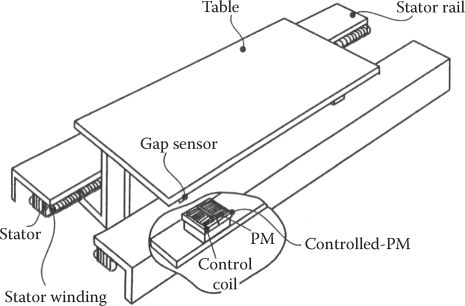
FIGURE 12.25 Industrial MAGLEV with four F-LPMSMs.

Images

FIGURE 12.26 Alternative for integrated levitation (and propulsion) control of F-LPMSM MAGLEV carrier.

The two control alternatives identified here are depicted in Figure 12.26.

It goes without saying that the addition of dc control coils may lead to probably better levitation control, but levitation control by $I_{d}^{*}$ control (by adding I_d dc regulators) may suffice in some applications.

Besides the here-suggested PI + SM (sliding mode) controllers for speed control plus P controller for position control and interior dc current regulators (Figure 12.24), recently fuzzy-neural-network controllers proposed to replace the position and speed cascaded controllers have been introduced [21,22]; Figure 12.27 [21].

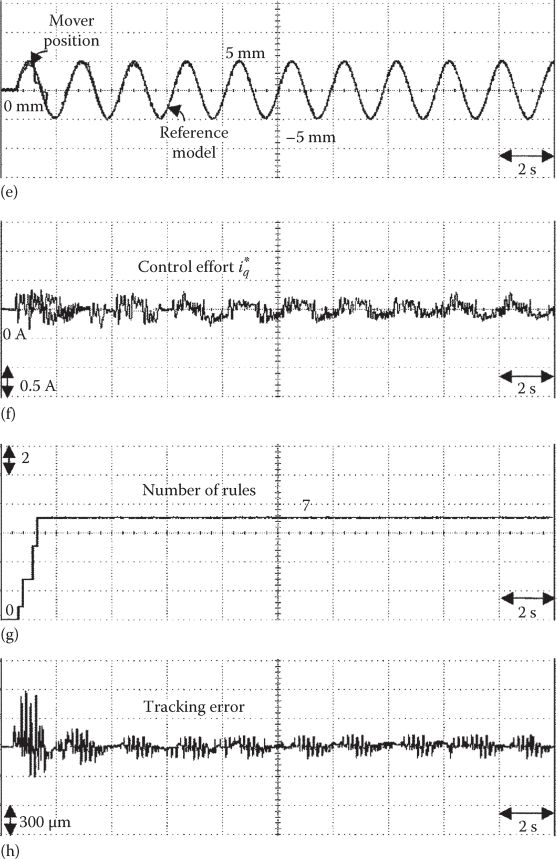
Sample results in Figure 12.28 show that the dynamic errors are still up to 0.2 mm for a trapezoidal periodic positioning of ± 5 mm with a period of 2 s [21]; and all these with position sensor resolution of a few μm.

Thrust pulsations due to nonsinusoidal emf, airgap variations, cogging force, and current ripple and vibration due to large normal force might be pertinent reasons why the dynamic positioning errors are still large.

Images

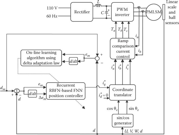
FIGURE 12.27 FOC with fuzzy neural network position control of F-LPMSMs. (After Lin, F.-J. et al., IEEE Trans., MAG-42(11), 3694, 2006.)

A way to reduce thrust total ripple, by cogging force pulsations compensation and using primary coordinates, is given in Ref. [23] (Figure 12.29); this may be a way to better dynamic position tracking with F-LPMSMs.

12.8.2 Direct Thrust and Flux (Levitation) Control (DTFC) of F-LPMSMs

In applications where thrust (rather than position or speed) tracking is required, direct flux and thrust estimation is performed; if the position feedback is available, the flux observer may be designed rather easily to work satisfactorily above 1-2 Hz; if position-sensorless control is required, then all the “arsenal” of motion sensorless control of rotary PMSMs may be “summoned to duty” for F-LPMSM [19,24]. Let us present such a generic position-sensorless DTFC system for F-LPMSM (Figure 12.30).

Images

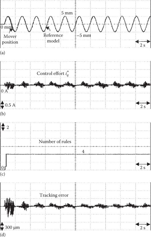
FIGURE 12.28 Test results with RBFM-based FNN position FOC of F-LPMSM. (After Lin, F.-J. et al., IEEE Trans., MAG-42(11), 3694, 2006.) (a) tracking response at nominal condition, (b) control effort at nominal condition, (c) number of rules at nominal condition, (d) tracking error at nominal condition. Test results with RBFM-based FNN position FOC of F-LPMSM. (After Lin, F.-J. et al., IEEE Trans., MAG-42(11), 3694, 2006.) (e) tracking response at parameter variation condition, (f) control effort at parameter variation condition, (g) number of rules at parameter variation condition, and (h) tracking error at parameter variation condition.

Images

For the primary flux ${\bar{ψ}}_{s}$ observer (Figure 12.31), we may use here a combined current and voltage model [18]:

${\bar{ψ}}_{S}^{s} = \int ({\bar{V}}_{S} - R_{S} {\bar{I}}_{S} + V_{c o m p}) d t (12.77)$

V_comp compensates the inverter nonlinearities and the primary resistor variations while it uses a PI loop on the error between the current and the voltage model (12.68), in stator coordinates, so as to produce both low-speed and higher-speed (frequency) primary flux good estimation (Figure 12.31).

Images

FIGURE 12.29 F-LPMSM vector control with $i_{d}^{*}^{'} = 0$ (a) and with cogging force compensation and (b) thrust and speed pulsation reduction (with $i_{d}^{*}^{'} = 0$ control) (c). (After Zeng, L. et al., IEEE Trans, MAG-46(3), 954, 2010.)

Images

FIGURE 12.30 Generic DTFC of LPMSM.

Images

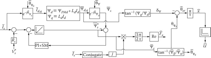
FIGURE 12.31 F-LPMSM state observer for sensorless DTFC: the primary flux ${\bar{ψ}}_{s}$ , thrust F_x, primary flux angle ${\overset{⌢}{θ}}_{ψ_{S}}$ , speed $\overset{⌢}{u}$ , and position $\overset{⌢}{x}$ (relative).

A few comments on DTFC are as follows:

The current to flux model (Figure 12.31) requires the stator flux angle ${\overset{⌢}{θ}}_{ψ_{S}}$ and is strictly valid in steady state; otherwise, the mover position angle ${\overset{⌢}{θ}}_{e r}$ may be used instead.
The speed $\overset{⌢}{u}$ is estimated from relative position $\overset{⌢}{x}$ by a time derivative; in reality, a PLL or other digital filter may be used to improve $\overset{⌢}{x}$ and obtain a better $\overset{⌢}{u}$ (speed estimation).
The relative position estimation $\overset{⌢}{x}$ may be used for drive positioning only if some proximity sensors exist along the track for periodic position calibration.
For initial position, or a nonhesitant start, a signal injection addition to $\overset{⌢}{x}$ is needed [19]. The primary flux amplitude control, Figure 12.30, is used to control the airgap (via normal force); a normal force estimator may also be added; then an additional normal force regulator is required before the stator flux ψ_S regulator.
The presence of PM flux makes the stator flux (and normal force) regulations (by I_d essentially) rather stiff but still worthy of consideration as no addition of power hardware is required for levitation control.
If cogging force cancelation is required, it is possible to add (−F_cog(x)) to $F_{x}^{*}$ and thus, with enough bandwidth in the thrust regulator, the F-LPMSM may compensate cogging force through the control system.
For industrial (low speed) travel (a few meters) with short primary mover MAGLEV carriers, it may be feasible to use interior PM fixed secondary with weaker PMs and higher magnetic saliency L_d/L_q ≥ 3 (airgap: 0.5 mm) (Figure 12.32).

Note on trapezoidal current control: As already discussed, both with air-core and iron-core primary, the emf may be trapezoidal (with q₁ = 1 and with q₁ < 0.5 (tooth-wound windings); in such cases, instead of sinusoidal current control (FOC or DTFC), trapezoidal (block) current control may be performed to avoid too large thrust pulsations, to better use the dc voltage coiling of the inverter, and to simplify the position (to proximity) sensor (three Hall sensors of low cost). To avoid repetition, this type of control will be treated in some detail in the next chapter, dedicated to tubular L-PMSMs.

Images

FIGURE 12.32 PM-assisted linear reluctance synchronous motor.

12.9 Design Methodology of L-PMSM by Example

Any design methodology starts with a set of specifications such as

Base continuum thrust: F_xn = 0.8 kN
Base speed: U_b=1.5 m/s
DC voltage: V_dc=300 V
Primary: as mover (short)
Normal force: zero (double-sided PM long secondary (stator))
Primary core: iron core
Airgap: g = 1 mm
Travel length: 3.5 m
Maximum speed: U_max = U_b = 1.5 m/s
Peak thrust at max. speed: F_xpeak = 1.2 kN
Efficiency at base power (1.2 kW) at base speed > 0.85
Power factor at base power (1.2 kW) at base speed > 0.8
Maximum ideal acceleration of primary a_max > 40 m/s²
Primary mover supply: by ac power flexible cable

What is required may be summarized as follows:

Use a realistic analytical model, size the PM long secondary and the short primary core.
Calculate, by the same model, the machine circuit parameters (inductances and resistances).
Use the circuit model (and vector diagrams) to calculate the performance at base (maximum) speed and base and peak thrust for V_dc=300 V.
Redo the process until all specifications are met.
Eventually, use a numerical code optimization design by choosing a variable vector, its domain of allowed values, and the aforementioned analytical model (or a more complex one) to evaluate a global objective function with constraints; then use an optimization algorithm (Hooke–Jeeves and genetic algorithms in [17]) to find an optimal design.

12.9.1 PM-Secondary Sizing

As there is no flux weakening in the design data (U_b = U_max), to yield good efficiency (high thrust/copper losses), surface PMs are planted on the two fixed long secondaries (stators); to reduce further thrust pulsations (cogging force), we use multiples of 6 slot/8 PM pole combinations for the primary/secondary and displace the two PM secondaries by 1/6 of a PM pole pitch (step skewing).

The primary teeth are premade and wound and fixed to a frame at stack ends; the bolts in the trapezoidal open holes are made of nonmagnetic material; the respective holes cause a further reduction of cogging force. Other manufacturing technologies of primary are feasible. As a 6 teeth (slot) primary/8 PM pole combination module is considered, the fundamental winding factor k_W₁=0.866. A 12 slot/10 PM pole module would have had k_W₁=0.933, both for a double and a single layer winding (as the one in Figure 12.33). The 2p > N_S (8/6) means less maximum PM flux per coil for larger thrust per given mmf than for the 4 PM pole, 6 slot case. Also, the yoke flux is smaller, so the stator yoke of fixed long secondary (stator) is thinner; consequently, cost is reduced notably. The machine has two airgaps, but this is “the price” for ideally zero normal force on primary movers.

Images

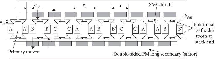
FIGURE 12.33 Double-sided F-LPMSM with primary mover (6 slots/8 PMs poles).

An FEM study considering variations for τ_PM/τ, τ_PM/τ_s, b_s₀/τ_s, g/h_m would lead to a practical design that mitigates between more average thrust density (N/cm²) at a good loss factor (N/W) with small enough cogging force. However, τ_PM ≈ (τ_s − b_s₀)0.8, τ = 30 mm, τ_s=τ • 2p/N_S=30 × 8/6=40 mm would be a good start (g = 1 mm, b_s₀=(3−4)g = 3−4 mm). After choosing the airgap PM flux density B_PMg = 0.7 T for a bonded NeFeB PMs with B_r=0.8 T, µ_rec = 1.07 μ₀, the PM height h_m is calculated from (12.65)

$\begin{array}{l} B_{P M g} \frac{π}{4} = B_{P M g u} = B_{r} \cdot \frac{h_{m}}{h_{m} + g} \cdot \frac{1}{1 + k_{f r i n g e}}; & \frac{h_{m}}{h_{m} + g} = \frac{0.7 \times 1.2 \times 4}{π0 .8} = 0.825 \end{array} (12.78)$

The fringing factor kf_ringe (due to loss of PM flux between teeth necks), for surface PMs, if b_s₀/g=4−5, kf_ringe ≤ 0.2 (it may be checked by FEM). B_PMgu is in fact the “useful” flux density that produces PM flux in the primary coils. For g = 1 mm, it follows that h_m = 5.7 mm. This rather thick PM leads also to smaller main inductance and thus to a better power factor (lower inverter kVA); since bonded NeFeB PMs are considered, their total cost should be reasonable. The PM span τ_PM = (τ_s − b_S₀) × 0.8 = (40 − 5)0.8 = 28 mm < τ=30 mm; the inter-PM space may be filled with adhesive to better fix the magnets.

The yoke of PM-secondary h_yS is

$h_{y S} \approx \frac{τ_{P M} \cdot B_{g P M u}}{B_{y S}} = 28 \times \frac{0.7}{1.7} = 11.5 mm (12.79)$

To allow for armature-reaction contribution at peak thrust, h_yS = 15 mm; solid mild steel may be used for PM-secondary yoke; the magnetic airgap (g + h_m) is large and thus the subharmonics flux of the primary mmf does no “reach” the solid yoke of stator to produce large eddy currents. Still to find is the primary stack length l_stack, almost equal to PM (and stack) length. Considering a base thrust density f_xb = 2 N/cm² (3 N/cm² for peak thrust) and an integer number of primary modulus, the thrust is

$F_{x n} = f_{x b} \cdot l_{s t a c k} \cdot 6 τ_{s} \cdot n (12.80)$

Hence, the choice between l_stack and number of primary-mover modules, n, depends on the secondary (travel) length, which, then, determines its initial costs. For a 4 m length track, the primary length could not be above 0.5 m (travel length 3 m); for n = 2, the primary length is 6τ_S • n = 6 × 40 × 2 = 480 mm = 0.48 m.

Consequentanly l_stack ^is

$l_{s t a c k} = \frac{800}{2 \times 10^{4} \times 0.48} = 0.0833 m (12.81)$

12.9.2 Primary Sizing

For U_b = 1.5 m/s and τ = 0.03 m, the base frequency f₁_b = 1.5/(2 × 0.03) = 25 Hz. Assuming that the PM flux linkage ψ_PMd in the primary coils (4 in all, in series per phase) varies sinusoidally with mover position, its peak value is approximately

$\begin{array}{l} ψ_{P M d} = B_{P M g u} τ_{P M g u} τ_{P M} l_{s t a c k} 4 W_{C} k_{W_{1}}; & p = 4 \end{array} (12.82)$

W_C is turns/coil

$ψ_{P M d} = 0.7 \times 0.028 \times 0.0833 \times 4 \times W_{C} \times 0.86 = 5.66 \times 10^{- 3} \cdot W_{C} = k_{P M} W_{C} (12.83)$

The rated (base) thrust F_xn is

$\begin{array}{l} F_{x n} = 800 = \frac{3}{2} \frac{π}{τ} ψ_{P M d} \cdot I_{q n} = \frac{3}{2} \frac{π}{0.03} \times 5.66 \times 10^{- 3} \times W_{C} \cdot I_{s n} \\ I_{q n} = I_{s n} (I_{d} = 0) \end{array} (12.84)$

So W_C • I_sn=900 A turns/coil (peak value). As there are two coils in a primary slot, the active area of the slot, A_slot is

$A_{s l o t} = \frac{2 W_{C} (I_{s n} / \sqrt{2})}{j_{C o} k_{f i l l}} = \frac{2 \times 900 / \sqrt{2}}{45 \times 0.4} = 792 {mm}^{2} (12.85)$

The slot width b_s ≈ 0.5τ_S=0.5 × 40=20 mm, so the active slot height h_su is

$h_{s u} = \frac{A_{s l o t}}{b_{s}} = \frac{792}{b_{s}} \approx 40 mm (12.86)$

Note: We have to add on each side of the doubly opened slot about 5 mm (h_ss=4 mm) of height, to leave room for the rods that support the primary cores.

The rated current density j_Con=4 A/mm² and the slot fill factor k_fill=0.4, as there is space between the two coils in slot.

There is no yoke in the primary mover, in order to reduce its weight.

12.9.3 Circuit Parameters and Vector Diagram

The synchronous inductance comprises the “magnetization” one L_m=L_dm=L_qm and the leakage one L_l. The magnetization inductance is straightforward (and apparently includes space harmonics contribution):

$\begin{array}{l} L_{m} \approx \frac{3}{2} \frac{μ_{0} (τ_{s} - b_{s 0}) l_{s t a c k} W_{C}^{2} 4}{4 (g + h_{m}) k_{C}}; & p = 4 = number of coils/phase \end{array} (12.87)$

$L_{m} = \frac{3}{2} \cdot \frac{1.256 \times 10^{- 6} \times (0.04 - 0.005) \times 0.0833 \times 4 \times W_{C}^{2}}{4 \times (1 + 5.7) 10^{- 3} \times 1.1} = 0.7453 \times 10^{- 6} \cdot W_{C}^{2} (12.88)$

The leakage inductance of the four coils per phase includes basically slot leakage and end coil leakage components:

$L_{l} = 4 \times 2 μ_{0} \cdot l_{s t a c k} (λ_{s l o t} + \frac{l_{e}}{l_{s t a c k}} \cdot λ_{e n d}) \cdot W_{C}^{2} (12.89)$

The slot is doubly opened and the variation of leakage field H along slot height is as in Figure 12.34.

The situation is equivalent to two semiclosed slots of half-height, but with doubled slot width:

$λ_{s l o t} \approx 2 (\frac{h_{s u}}{3 \cdot (2 \cdot b_{s})} + \frac{h_{s s}}{b_{s} + b_{s 0}}) = 2 (\frac{\frac{40}{2}}{3 \times 2 \times 20} + \frac{4}{20 + 5}) = 0.652! (12.90)$

The end coil geometrical permeance λ_e ≈ 0.63 (as in q = 1 windings) [19].

$L_{l} = 4 \times 2 \times 1.256 \times 10^{- 6} \times 0.0833 \times (0.652 + \frac{1.2 \times 0.04}{0.0833} \times 0.33) \cdot W_{C}^{2} = 0.7049 \times 10^{- 6} \cdot W_{C}^{2} (12.91)$

As seen L_l ≈ L_m, since the machine has four large equivalent airgaps per flux closed path. So L_s=L_m+L_l = 1.45 × 10⁻⁶ W_C².

The phase resistance R_S is simply

$R_{S} = 4 ρ_{c o} l c \frac{W_{c}^{2} j_{c o n}}{W_{C} I_{s n} / \sqrt{2}} = 4 \times 2.1 \times 10^{- 8} \times 0.2826 \frac{4 \times 10^{6}}{900 / \sqrt{2}} \cdot W_{C}^{2} = 1.4876 \times 10^{- 4} \cdot W_{C}^{2} = k_{R} \cdot W_{C}^{2} (12.92)$

$l_{C} \approx 2 \cdot (l_{s t a v k} + 1.2 \cdot τ_{s} + 0.01) = 2 \cdot (0.0833 + 1.2 \times 0.04 + 0.01) = 0.2826 m (12.93)$

As the f₁_b=25 Hz, the core losses are to be notably smaller than copper losses (less than 1 W/kg at 1.5 T and 25 Hz). Standard transformer (oriented grain) laminations (0.35 mm thick) may be used.

The vector diagram “spells” the voltage equation (Figure 12.35):

$\begin{array}{l} {\bar{V}}_{S 0} = R_{S} {\bar{I}}_{S 0} + j \frac{π}{τ} (U k) {\bar{ψ}}_{S}; & {\bar{ψ}}_{S} = ψ_{P M d} + j L_{q} I_{q}; & I_{d} = 0 \end{array} (12.94)$

Images

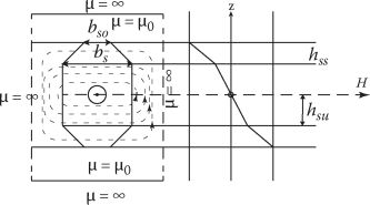
FIGURE 12.34 Slot leakage field.

Images

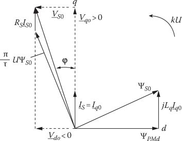
FIGURE 12.35 F-PLMSM vector diagram at steady state with I_d=0.

$\begin{array}{l} V_{d 0} = R_{S} I_{d 0} - \frac{π}{τ} (U k) L_{q} I_{q 0} \\ V_{q 0} = R_{S} I_{q 0} + \frac{π}{τ} (U k) ψ_{P M d} \\ V_{S 0} = \sqrt{V_{d 0}^{2} + V_{q 0}^{2}} \end{array} (12.95)$

k = 1 for PM mover

k = −1 for primary mover

12.9.4 Number of Turns per Coil W_L and Wire Gauge d_Co

To calculate the number of turns W_l, we have to “test” the vector diagram at peak thrust (rather than base thrust) at maximum voltage V_{s max}:

$V_{s \max} \approx \frac{2 V_{d c}}{π} \cdot 0.95 = \frac{2 \times 300}{π} \times 0.95 = 181.52 V (peak phase valu) (12.96)$

For 1200 N of thrust W_C • I_Speak = 1.5 • W_C • I_Sn = 900 × 1.5 = 1350 A-turns (peak value per coil); there are four coils in series per phase. Knowing the parameters’ expressions (but W_C), we may now use the vector diagram:

$\begin{array}{l} V_{s \max} = W_{C} \sqrt{{(k_{P M} \frac{π}{τ} \cdot U + k_{R} (W_{C} \cdot I_{s p e a k}))}^{2} {(\frac{π}{τ} \cdot U \cdot k_{L} W_{C} \cdot I_{s p e a k})}^{2}} \\ V_{s \max} = W_{C} \sqrt{{(5.66 \times 10^{- 3} \times \frac{π}{0.03} \times 1.5 + 10^{- 4} 1.4876 \times 1350)}^{2} + {(\frac{π}{0.03} \times 1.5 \times 1.45 \times 10^{- 6} \times 1350)}^{2}} \\ = W_{C} \sqrt{{1.08944}^{2} + {0.3073}^{2}} = W_{C} \cdot 1.132 \end{array} (12.97)$

$W_{C} = \frac{181.52}{1.132} = 160 turns/coil$

$\begin{array}{l} W_{C} I_{s n} = 900; & I_{s n} = \frac{900}{160} = 5.666 A; & I_{n} = \frac{I_{s n}}{\sqrt{2}} = 4.014 A (RMS per phase) \end{array} (12.98)$

With j_Con=4 A/mm², the wire diameter is

$d_{C o} = \sqrt{\frac{4}{π} \cdot \frac{I_{n}}{j_{c o n}}} = \sqrt{\frac{4}{π} \times \frac{4.014}{4}} = 1.13 mm (bare wire) (12.99)$

12.9.5 Efficiency, Power Factor, and Voltage at Base Thrust

At base thrust the phase current I_n=4.014 A, and thus the copper losses are

$p_{C o n} = 3 R_{S} I_{n}^{2} = 3 \times 1.4876 \times 10^{- 4} \times {(\frac{900}{\sqrt{2}})}^{2} = 180.7 W (12.100)$

So the efficiency at rated thrust is

$η_{n} = \frac{F_{x n} U_{b}}{F_{x n} U_{b} + p_{C o n}} = \frac{800 \times 1.5}{1200 + 180.74} = 0.869 > 0.85 (12.101)$

Given the low speed (1.5 m/s), the efficiency, for 2 N/cm² thrust density, is considered really good.

The power factor can be calculated from (12.87) with W_CI_sb = W_CI_peak × 2/3; with W_C known, the voltage V_S can be obtained from (12.97):

$\begin{array}{l} V_{S} = 160 \sqrt{{(5.66 \times 10^{- 3} \times \frac{π}{0.03} \times 1.5 + 10^{- 4} \times 1.486 \times 900)}^{2} + {(\frac{π}{0.03} \times 1.5 \times 1.45 \times 10^{- 6} \times 900)}^{2}} \\ = 160 \sqrt{{1.02248}^{2} + {0.20488}^{2}} = 160 \times 1.0428 = 166.848 V (peak phase value) \end{array} (12.102)$

The power factor may be calculated simply as

$\cos φ_{n} = \frac{1.02248}{1.0428} = 0.98 (12.103)$

Even for peak thrust the copper losses are

$p_{C o p} = p_{C o n} {(\frac{F_{x p e a k}}{F_{x n}})}^{2} = 180 \times {(\frac{3}{2})}^{2} = 405 W (12.104)$

$η_{p e a k t h r u s t} = \frac{1200 \times 1.5}{1800 + 405} = 0.816 (12.105)$

And from (12.87)

$\cos φ_{p e a k} = \frac{1.0814}{1.132} = 0.955 (12.106)$

12.9.6 Primary Active Weight

The primary active weight is made of core weight W_core and copper weight W_Copper:

$\begin{array}{l} W_{c o r e} = 12 l_{t a c k} [τ_{s} \cdot (h_{s u} + 2 h_{s s}) - (h_{s u} \cdot b_{s} + (b_{s} + b_{S 0}) h_{s s})] γ_{i r o n} \\ = 12 \times 0.0833 \times [0.04 \times (0.04 + 2 \times 0.005) - (0.04 \times 0.02 + (0.02 + 0.005) \times 0.005)] \\ \times 7600 = 8.138 kg \end{array} (12.107)$

$\begin{array}{l} W_{c o p p e r} = \frac{3 \times l_{c} W_{c} \times 4 \times I_{n} γ_{C o}}{j_{C o n}} = \frac{3 \times 0.286 \times 160 \times 4 \times 4.014 \times 8900}{(4 \times 10^{6})} \\ = 4.846 kg \end{array} (12.108)$

$W_{a p} = W_{c o r e} + W_{C o p p e r} = 8.138 + 4.846 = 12.98 kg (12.109)$

Let us suppose that the primary framing and rolling facility of mover leads to a total mover weight W_mover=20 kg. Consequently, the ideal maximum acceleration (available up to base (maximum) speed of 1.5 m/s for F_xpeak = 1200 N) is

$a_{i \max} = \frac{1200}{20} = 60 {m/s}^{2} \approx 6 \cdot a_{g r a v i t y} > > 40 {m/s}^{2} (12.110)$

12.9.7 Design Summary

Primary (mover) active and total weight: 12.98 kg/20 kg.
Maximum ideal acceleration (up to 1.5 m/s) is 60 m/s².
The efficiency and power factor at rated thrust 800 N and U_b are 0.869 and 0.98, respectively, f_n=25 Hz, V_sn = 161.848 V (peak phase value).
For the peak thrust (1200 N) and U_b = 1.5 m/s at V_s_max = 181.52 V (V_dc ≈ 300 V), efficiency is still 0.816 and the power factor is still very good: 0.955.
The rather very good power factor is due to the small fundamental frequency f_n = 25 Hz, and due to the small machine inductance L_S = 1.45 × 10⁻⁶ × 160² = 37.12 mH; the stator resistance R_S = 1.4876 × 10⁻⁴ × 160² = 3.808 Ω.
In turn L_S is small due to the large total magnetic airgap 4(g+h_m) and small leakage inductance due to doubly opened slots and short end-coils (small pole pitch).
As power factor is high, the design at higher thrust for higher current density, smaller number of turns, but lower efficiency is also possible.
It is quite disputable that such performance, at such a low speed, can be surpassed in aggregated performance by many other configurations.

12.9.8 Note on F-LPMSM as Three-Phase Generators

For wave generators, speeds in the range of 0.7–1.5 m/s are required for very large thrust (tens of kN for tens of kW and hundreds of kN for hundreds of kW) for short (a few meters) travel length. For such designs, square-shape (four-sided) F-LPMSM has been proposed for 16 kW generators with PM-mover, operating at 10 Hz for 0.9 m/s [25]. As the thrust density for rather small pole pitch (τ=45 mm) is not very high—as seen earlier, the weight and cost of the device are still large. A 250 kW (speed around 1 m/s) F-LPMSM wave generator has been calculated in [26]. It uses a tooth-wound winding in the double-sided short stator and double-sided PM long mover (translator) with interior PMs. By proper skewing with semiclosed stator slots, the cogging force was reduced to well below 1% of rated thrust. However, at moderate pole pitch (in latter case [26] τ = 60 mm in the PM mover) and slot pitch τ_s = 165 mm!) and such a small speed, it is still hard to say that q = 1 or q < 0.5 winding stator configurations will result in acceptable power/weight and efficiency for large wave generators. Shifted tooth wound τ=τ_s primaries (by half slot pitch) pitch phase double-sided modules for F-LPMSM have been proven to allow larger thrust density with low armature reaction [27] and may constitute a way to lower weight for such large thrust for reasonable generator weight cost, efficiency, and power factor (which influences heavily the PWM inverter kVA ratings and cost).

12.10 Summary

Linear PM synchronous motors are the counterparts of the rotary PM synchronous machine, which are characterized essentially by sinusoidal emf and thus by sinusoidal current control.
The primary has a three-phase ac winding area built with distributed coils (q ≥ 1) or tooth-wound (nonoverlapping) coils (q ≤ 0.5), placed in the uniform slots of a laminated iron core or in an air (plastic) core.
The primary may be the stator, placed along the track, or the mover; in the latter case, the electric power is transferred to the mover by sliding power collector (pantographs) or by flexible power cable for short travel.
The PM secondary or primary may be the mover.
To cancel the normal force, double-sided primaries or secondaries are used.
To calculate the emf thrust F_x and normal force F_n, typical to flat linear PM synchronous motors (F-LPMSMs), a 2(3) D multilayer analytical field model is first applied; even slot openings can be considered by defining a proper inverse-airgap function.
Also 2(3) D magnetic equivalent circuit (MEC) methods are used to fully characterize F-LPMSMs, including magnetic saturation, besides all geometry parameters (and slot openings).
These two methods allow to calculate emfs, force, and inductances —circuit parameters—to prepare all data for phase variable and then for the dq model of F-LPMSMs.
In addition, the moderate computation time of multilayer methods recommends them for optimization design methodologies.
For “ultimate” precision, 2(3) D-FEM is used (in its magnetostatic, time stepping, and field-circuit modes) to describe F-LPMSM; the only trouble is the computation time; to check (and correct) or to perform direct geometric optimization design around the analytical optimum design, FEM is the way to go.
Field theories yield the data (dB/dt in essence) for calculation of core losses.
F-LPMSM with iron-core primary experience a longitudinal force at zero current, called cogging force (the counterpart of cogging torque in rotary PM machines); it is caused by the variation of coenergy stored in the PMs with slot openings; as expected its average is practically zero; the cogging force pulsates at the number of periods equal to LCM (N_slots, 2p PM poles); the larger the LCM, the smaller the cogging force peak.
Methods to reduce cogging force [28] are similar to those used in rotary machines: PM span/pole/pitch ratio, PM poles displacement, skewing, end-teeth shaping etc; besides, thrust ripple disturbance rejection by control is also feasible [29].
The dq model of F-LPMSM can include not only the propulsion motion (horizontal, in general) but also the levitation motion (vertical, in general along airgap).
There are two FOC methods for F-LPMS control: zero I_q propulsion control and, respectively, flux weakening ( $I_{d}^{*} < 0$ control) and thrust (I_q control); alternatively, $I_{d}^{*}$ can be used to control the levitation.
The structural diagrams for constant I_d (zero or not) and FOC of F-LPMSMs are very similar to that of PM brush motor, ideal for motion control.
On the other hand, primary thrust and flux control (DTFC) allow direct thrust control and it may be used to control levitation by flux control.
Advanced fuzzy neural network and other robust linear position tracking with F-LPMSM have shown very good steady-state precision but with still large dynamic tracking errors. Using a disturbance force, the observer may substantially enhance relative position tracking by F-LPMSM [30].
A DTFC for F-LPMSM without a position sensor reveals the possibility of even position sensorless tracking if a few calibration proximity position sensors are placed at known points along the track.
A design methodology with a case study for 1200 N (peak value up to 1.5 m/s) shows efficiency above 80%, a very good power factor for a 13 kg active weight (20 kg total) primary mover.
As recent research efforts have shown, the application of F-LPMSM as wave generators is thoroughly investigated (at about 1 m/s) and for 250 kW at 250 kN); the power/weight and efficiency and power factor product need further drastic improvements, before becoming economical.
New configurations with ever better performance keep surfacing [31–33].

References

1. Z. Deng, I. Boldea, and S.A. Nasar, Fields in PM-LSMs, IEEE Trans., MAG-22, 1986, 107–112.

2. Z. Deng, I. Boldea, and S.A. Nasar, Forces and parameters of PM-LSMs, IEEE Trans., MAG-23, 1987, 305–309.

3. Z.Q. Zhu, D. Howe, E. Bolte, and B. Ackerman, Instantaneous magnetic field distribution in brushless PM dc motors, Parts I-IV, IEEE Trans, MAG-29(1), 1993, 124–158.

4. V. Ostovic, Dynamics of Saturated Electric Machines, John Wiley & Sons, New York, 1989.

5. W.B. Jang, S.-M. Jang, and D.-Y. Yon, Dynamic drive analysis through base speed determination for optimum control boundary in PMLSM with self-load, IEEE Trans., MAG-41(10), 2005, 4027–4029.

6. D.L. Trumper, W.-J. Kim, and M.E. Williams, Design and analysis framework for linear PM motors, IEEE Trans, IA-32(2), 1996, 371–379.

7. B. Sheikh-Ghalavand, S. Vaez-Zadeh, and A.H. Isfahani, An improved magnetic equivalent circuit model for iron-core linear permanent magnet synchronous motors, IEEE Trans., MAG-46(1), 2010, 112–120.

8. I. Boldea, S.A. Nasar, and Z. Fu, Fields forces and performance of air-core linear self-synchronous motor with rectangular current control, IEEE Trans, MAG-24, 1988, 2194–2203.

9. T.J.E. Miller, Brushless PM and Reluctance Motor Drives, Oxford University Press, Oxford, U.K., 1989.

10. N. Baatar, H.S. Yoon, M.T. Pham, P.S. Shin, and C.S. Koh, Shape optimal design of a 9 slot 10 pole PM LSM for detent force reduction using adaptive response surface method, IEEE Trans, MAG-45(10), 2009, 4562–4565.

11. D.-Y. Lee, Ch.-G. Jung, K.-I. Yoon, and G.T. Kim, A study on the efficiency optimum design of a PM type LSM, IEEE Trans, MAG-41(5), 2005, 1860–1863.

12. S. Chaithongsuk, N. Takorabet, and F. Meybody-Tabar, On the use of PWM method for the elimination of flux density harmonics in the airgap of surface PM motors, IEEE Trans., MAG-45(3), 2009, 1736–1739.

13. J. Gieras, Linear Synchronous Motors, Chapter 5, CRC Press, Boca Raton, FL, 2000 (second edition, 2010).

14. B.-Q. Kou, W.H. Xing, L.-L. Yi, Z.-L. Liang, Z. Zhe, and C.-H. Chuan, The thrust characteristics investigation of double sided PMLSM for EML, IEEE Trans, MAG-45(1), 2009, 501–505.

15. G. Henneberger and C. Reuber, A linear synchronous motor for a clean room system, Record of LDIA-1995, Nagasaki, Japan, 1995, pp. 227–230.

16. I. Boldea and V. Coroban, BEGA—Vector control for wide constant power speed range at unity power factor, Record of OPTIM-2006, Brasov, Romania, 2006 (IEEExplore).

17. I. Boldea and L. Tutelea, Electric Machines: Steady State, Transients and Design with Matlab, Chapters 6 and 9, CRC Press, Taylor & Francis, New York, 2009.

18. I. Boldea and S.A. Nasar, Linear Motion Electromagnetic Devices, Chapter 4, Taylor & Francis Group, New York, 2001.

19. I. Boldea and S.A. Nasar, Electric Drives, 2nd edn., Chapters 10 and 11, CRC Press, Taylor & Francis Group, New York, 2009.

20. K. Yoshida, Y. Tsubone, and T. Yamashita, Propulsion control of controlled PMLSM Maglev carrier, Record of ICEM-1992, Manchester, U.K., 1992, pp. 726–740.

21. F.-J. Lin, P.-H. Shen, S.-L. Yang, and P.-H. Chou, Recurrent radial basis function network-based fuzzy neural network control for PMLSM servodrive, IEEE Trans., MAG-42(11), 2006, 3694–3705.

22. F.-J. Lin, P.-H. Shen, S.-L. Yang, and P.-H. Chou, Recurrent functional-link-based fuzzy neural network controller with improved particle swarm optimization for a linear synchronous motor drive, IEEE Trans., MAG-45(8), 2009, 3151–3165.

23. L. Zeng, X. Chen, X. Luo, and X. Li, A vector control method of LPMBDCM considering effects of PM flux linkage and cogging force, IEEE Trans., MAG-46(3), 2010, 954–959.

24. R. Krishnan, Permanent Magnet Synchronous and Brushless Motor Drives, CRC Press, Taylor & Francis, New York, 2010.

25. N.M. Kionoulakis, A.G. Kladas, and J.A. Tegoupoulos, Power generation optimization from sea waves by using PM linear generator drive, IEEE Trans., MAG-44(6), 2008, 1530–1533.

26. J. Faiz, M.E. Salari, and G. Shahgolian, Reduction of cogging force in linear PM generators, IEEE Trans., MAG-46(1), 2010, 135–140.

27. W.R. Canders, F. Laube, and H. Mosebach, High thrust double sided permanent magnet excited linear synchronous drive with shifted stators, Record of LDIA-2001, Nagano, Japan, 2001, pp. 435–440.

28. Y.-J. Kim, M. Wataba, and H. Dohmeki, Reduction of cogging force at the outlet edge of a stationary discontinuous primary linear synchronous motor, IEEE Trans, MAG-43(1), 2007, 40–45.

29. Y.-W. Zhu and Y.-H. Cho, Thrust ripples suppression of permanent magnet linear synchronous motor, IEEE Trans, MAG-43(6), 2007, 2537–2539.

30. Y.-D. Yoon, E. Jung, and S.-K. Sul, Application of a disturbance observer for a relative position control system, IEEE Trans, IA-46(2), 2010, 849–856.

31. Y. Du, K.T. Chau et al., Design and analysis of linear stator PM vernier machines, IEEE Trans, MAG-47(10), 2011, 4219–4222.

32. G. Zhou, X. Huang, H. Jiang, L. Tan, and J. Dong, Analysis method to a Halbach PM ironless linear motor with trapezoidal windings, IEEE Trans., MAG-47(10), 2011, 4167–4170.

33. C.-C. Hwang, P. Li, and C.-T. Liu, Optimal design of a PM-LSM with low cogging force, IEEE Trans., MAG-48(2), 2012, 1039–1042.

..................Content has been hidden....................

You can't read the all page of ebook, please click here login for view all page.

Table of Contents for Chapter 12 Flat Linear Permanent Magnet Synchronous Motors

Create new playlist

Sign In

Sign Up

Table of Contents for
Chapter 12 Flat Linear Permanent Magnet Synchronous Motors