Chapter 5 Design of Flat and Tubular Low-Speed LIMs

Search in book...
Toggle Font Controls
Create new playlist

Name your new playlist

Playlist description (optional)
Sign In

Email address

Password

Forgot Password?

or

Continue with Facebook

Continue with Google
Sign Up

Full Name

Email address

Confirm Email Address

Password

or

Continue with Facebook

Continue with Google

Low-speed LIMs are LIMs whose dynamic end effects can be neglected [(γ₂_r τ)⁻¹ < 2 p/10] (as described in Chapter 3). They have to be designed, consequently, for a goodness factor less than the optimum value G_e₀ (Chapter 3), which varies linearly with the number of poles 2p (G_e = 10 for 2p = 4 and G_e = 40 for 2p = 16).

Though we are intuitively tempted to assimilate low speed with low goodness factor and thus end effect neglection, the situation is more complex, as in principle we could obtain the same equivalent goodness factor G and thus the same end effect (for the given pole count and slip), for up to 3/1 speed ratio [1].

So, we should choose for a low-speed application a low goodness factor (with negligible end effect) or, better, an optimal goodness factor design, which shows some end effect, but for better overall performance (thrust density, efficiency, and power factor)? The answer to this question is related to the application, as higher G_e means inevitably higher pole pitch, which means thicker back iron both in the primary and secondary of SLIMs (the favorite practical topology) and higher initial costs of SLIM.

Therefore, the “low-speed LIM” concept is just a simplified design option based on the strong similarities with rotary IM design methodologies, which constitute a valuable heritage to use for the scope.

In fact the “low-speed LIM” design concept may be the first (very preliminary) design step for any LIM (even for high speed) to get a strong feeling of magnitudes in the absence of a vast industrial experience data, as for rotary IMs.

By design we mean here “dimensioning” or “sizing,” which is the finding of complete manufacturing data (geometry, parameters, and performance characteristics) to meet initial specifications, by using adequate LIM analytical (or numerical) field and circuit models. This operation is a synthesis while using a given geometry of LIM to calculate circuit parameters, and performance is, in fact, an analysis stage.

Optimization design means repetitive usage of design to comply best with initial specifications based on a multiobjective function (with constraints) and a mathematical algorithm to obtain convergence within reasonable computation effort (time). The design refers to three main aspects:

Electromagnetic
Thermal
Mechanical

In what follows we will refer only to electromagnetic design. As for thermal and mechanical design, we will only limit current and flux densities and the shear stress components (propulsion and normal surface force densities in N/cm²) to make sure they comply with standard material properties.

A complete thermal and mechanical design of LIMs (based on analytical and (or) on finite element multilayer model) is beyond our scope here. To save space we will unfold analytical electromagnetic design methodologies for

Flat SLIMS with ladder secondary
Tubular SLIMS with ladder secondary, for speeds below 10 m/s and negligible dynamic end effect conditions, and travel lengths of 1–2 m travel for tubular SLIMS in industry, and tens of meters for other, special, applications.

The aluminum sheet on iron secondary SLIM has been proven to yield poor performance (η₁ cos φ₁ < 0.2–0.3) [2] for low-speed applications, and thus, in the presence of strong competition of linear permanent magnet (or dc-excited) synchronous motors (LSMs), it will not be treated here further. However it will be considered for medium- and high-speed LIMs because of lower cost of the long secondary (track) for long travels, despite lower η₁ cos φ₁ (0.4–0.45) than for LSMs (η₁ cos φ₁ < 0.6–0.7), which implies higher KVA (and costs) PWM inverter supplies in the overall cost of the system (such as net present worth). The costs of the secondary (track) for long travels (tens and hundreds of kms) retain a very important share. To keep the presentation closer to the scope, we will present the design methodologies by numerical examples. The optimization design will be addressed only for medium to high speed (transportation LIMs in Chapter 6). We should emphasize that the LIM design methodology here revolves around the equivalent goodness factor concept. And it is based on 1D analytical field theory, which includes slot opening, magnetic saturation, and edge and skin effects by correction coefficients, as a basis to define the parameters of the standard IM equivalent circuit. The parameters expressions, however, are related to LIM topology and vary with primary mmf and slip frequency via equivalent goodness factor.

Alternative design methodologies are available elsewhere [2].

5.2 Flat SLIM with Ladder Long Secondary and Short Primary

The electromagnetic design of LIMs is related strongly to the application, due to the absence of any mechanical transmission between the latter and the load.

Let us consider here a machine-tool table application with the following general specifications:

1. Specifications

Rated thrust: F_xn=500 N

Maximum travel length: l_travel = 3 m

Rated speed: u_n=3 m/s

Power source: three-phase ac 220 V/60 Hz line voltage, with diode rectifier and PWM voltage source IGBT inverter

Some additional data from previous experience are added as follows:

2. Additional experience-based data

The mechanical airgap, with linear bearings, may be chosen as low as g = 1.0 mm, especially if the host primary mover is placed below the ladder secondary (stator) such that the large normal force F_n covers most of the mover total weight (by adequate F_n control); in the latter case, the stress of linear bearings becomes notably smaller than usual.
The allowance for normal force leads to the possibility of choosing a large rated airgap flux density (B_g₁_n = 0.55 − 0.7 T), not larger, to avoid heavy magnetic saturation of laminated cores of primary and secondary.
Slot shape factor h_s₁/b_s ≈ 4–6 in the primary, lower in the secondary, with slot openings b_s₁/g < 6 and b_s₂/g < 4, to keep the leakage inductances of primary and secondary within bounds and, at the same time, reduce Carter coefficient and surface core losses (due to slot space harmonics field); see Figure 5.1.
The primary winding may be single layer (with q₁ = 1 slot/pole/phase or q′₁ = 2 for lower the mmf. space harmonics), and thus lower the additional cage and core surface eddy current losses, when the number of primary slots N_s₁ = 2pq₁ it may be also 2 layer type with q₁ = 1, 2 and (eventually) chorded coils (x/τ = 5/6 for q₁ = 2). For 2p + 1 poles in the primary (with half-filled end pole slots), the coils are shorter so the copper is better used, but primary core is longer (by almost one pole) and thus not completely used. We will choose here 2p poles single-layer, full pitch, (q₁ = 2) primary winding, with the slot pitch τ_s1.
The number of poles 2p is still to be chosen but 2p > 4, to avoid asymmetrical phase currents due to static end effect.
The slot pitch in the secondary τ_s₂ should be different from τ_s₁ (in the primary), but not far from each other (as for rotary IMs), to avoid notable thrust pulsations.
The key dimensioning (sizing) factor considered here is the shear secondary stress: for free air coiling f_xn = F_xn/(primary area) ≈ 1 N/cm² and 1.5–2 N/cm² for forced air cooling. This value interval of f_xn is justified only by the rather small airgap and the ladder secondary (for Al-on-iron secondary SLIMs f_xn is smaller for low-speed applications).
As we make use of the rotary IM equivalent circuit (Figure 5.2), we gather here the expressions of circuit parameters (as developed in Chapter 4, [4,5]):

Images

FIGURE 5.1 Flat primary and secondary slot geometries. (After Boldea, I. and Nasar, S.A., Linear Electric Actuators and Generators, Cambridge University Press, Cambridge, U.K., 1997.)

The primary resistance per phase:

R 1 = 2 ρ C o ( l s t a c k + l e c ) j c o r w 2 1 w 1 I 1 r (5.1)

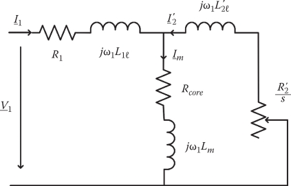
$R_{1} = \frac{2 ρ_{C o} (l_{s t a c k} + l_{e c}) j_{c o r} w_{1}^{2}}{w_{1} I_{1 r}} (5.1)$

Images

FIGURE 5.2 Low-speed equivalent circuit per phase.

Primary leakage inductance:

L 1 l = 2 μ 0 p q 1 ((λ s 1 + λ d i f f 1) l s t a c k + λ e c 1 l e c) w 1 (5.2)

$L_{1 l} = \frac{2 μ_{0}}{p q_{1}} ((λ_{s 1} + λ_{d i f f 1}) l_{s t a c k} + λ_{e c 1} l_{e c}) w_{1} (5.2)$

Slot specific (nondimensional) permeance:

λ s 1, 2 = h s 1, 2 ( 1 + 3 β ) 12 b s 1 , 2 + h s p , s b s p , s (5.3)

$λ_{s 1, 2} = h_{s 1, 2} \frac{(1 + 3 β)}{12 b_{s 1, 2}} + \frac{h_{s p, s}}{b_{s p, s}} (5.3)$

Airgap leakage specific permeance:

λ d i f f 1, 2 \approx 5 K c g / b s p , s 5 + 4 ( K c g / b s p , s ) (5.4)

$λ_{d i f f 1, 2} \approx \frac{5 K_{c} g / b_{s p, s}}{5 + 4 (K_{c} g / b_{s p, s})} (5.4)$

Primary end-coil leakage specific permeance:

λ e c 1 = 0.3 (3 β - 1) q 1 (5.5)

$λ_{e c 1} = 0.3 (3 β - 1) q_{1} (5.5)$

The magnetization inductance:

L m = 6 μ 0 ( K w 1 w 1 ) 2 τ l s t a c k π 2 K c g p ( 1 + K s s ) (5.6)

$L_{m} = \frac{6 μ_{0} {(K_{w 1} w_{1})}^{2} τ l_{s t a c k}}{π^{2} K_{c} g p (1 + K_{s s})} (5.6)$

Secondary resistance (referred to primary):

R' 2 = 12 ρ A l ( K w 1 w 1 ) 2 N s 2 (l s t a c k A s 2 + 2 l l a d A l a d) (5.7)

${R^{'}}_{2} = 12 ρ_{A l} \frac{{(K_{w 1} w_{1})}^{2}}{N_{s 2}} (\frac{l_{s t a c k}}{A_{s 2}} + \frac{2 l_{l a d}}{A_{l a d}}) (5.7)$

N_s₂ is the secondary slots/primary length.

Secondary leakage inductance (referred to primary):

L' 2 l \approx 24 μ 0 l s t a c k (λ s 2 + λ d i f f 2) ( K w 1 w 1 ) 2 N s 2 \times (1 + K l a d d e r) (5.8)

${L^{'}}_{2 l} \approx 24 μ_{0} l_{s t a c k} (λ_{s 2} + λ_{d i f f 2}) \frac{{(K_{w 1} w_{1})}^{2}}{N_{s 2}} \times (1 + K_{l a d d e r}) (5.8)$

with

A l a d = A s 2 2 sin ( α e s / 2 ); α e s \approx 2 π p N s 2; l l a d \approx 2 p τ N s 2; A s 2 = h s 2 \cdot b s 2 (5.9)

$A_{l a d} = \frac{A_{s 2}}{2 \sin (α_{e s} / 2)}; α_{e s} \approx \frac{2 π p}{N_{s 2}}; l_{l a d} \approx \frac{2 p τ}{N_{s 2}}; A_{s 2} = h_{s 2} \cdot b_{s 2} (5.9)$

Other symbols in (5.1) through (5.9) are as follows:

l_stack—primary (and secondary) stack width
g—mechanical gap
K_c—Carter coefficient for dual slotting
l_ec—end-coil length per side; l_ec ≈ ∼0.01 + 1.5y (y-coil span); β = y/τ = 1 or 5/6 etc.; τ—pole pitch

Note: Similar expressions are valid for Al-on-iron, with g + d_Al instead of g, d_Al—aluminum thickness such as N_s₂A_s₂=2pd_Alτ; ρ_Al is augmented by the edge effect coefficient K_tr > 1 and reduced by the contribution of solid back in thrust; the magnetic saturation factor K_s accounts for secondary back iron and primary teeth and back-iron contribution to magnetization current (Chapters 3 and 4).

3. Primary sizing

For start we lump by coefficient K_l₂ the secondary leakage inductance (L′₂_l) influence, and thus the airgap flux density (3.24) is

B g 1 = μ 0 K e = μ 0 J 1 m π τ g K c ( 1 + K s ) 1 + s 2 G e 2 - - - - - - - - \sqrt = μ 0 θ 1 m g K c ( 1 + K s ) 1 + s 2 G e 2 - - - - - - - - \sqrt (5.10)

$B_{g 1} = μ_{0} K_{e} = \frac{μ_{0} J_{1 m}}{\frac{π}{τ} g K_{c} (1 + K_{s}) \sqrt{1 + s^{2} G e^{2}}} = \frac{μ_{0} θ_{1 m}}{g K_{c} (1 + K_{s}) \sqrt{1 + s^{2} G e^{2}}} (5.10)$

with the primary mmf/pole θ₁_m (as for rotary IMs)

θ 1 m = 3 2 - \sqrt ( K w 1 ω 1 ) I 1 π p (5.11)

$θ_{1 m} = \frac{3 \sqrt{2} (K_{w 1} ω_{1}) I_{1}}{π p} (5.11)$

and

(G e i) = ω 1 L m / (R' 2 \cdot K l 2) \approx μ 0 ω 1 τ 2 σ A l h s 2 ( 1 - b s 2 / τ s 2 ) π 2 g K c ( 1 + K s ) K r \cdot K l 2 K r = 1 + L l a d A l a d \cdot A s 2 l s t a c k; K l 2 = 1 + (ω 2 L ' 2 l R ' 2) 2 - - - - - - - - - - \sqrt (5.12)

$\begin{array}{l} (G_{e i}) = ω_{1} L_{m} / ({R^{'}}_{2} \cdot K_{l 2}) \approx \frac{μ_{0} ω_{1} τ^{2} σ_{A l} h_{s 2} (1 - b_{s 2} / τ_{s 2})}{π^{2} g K_{c} (1 + K_{s}) K_{r} \cdot K_{l 2}} \\ K_{r} = 1 + \frac{L_{l a d}}{A_{l a d}} \cdot \frac{A_{s 2}}{l_{s t a c k}}; K_{l 2} = \sqrt{1 + {(\frac{ω_{2} {L^{'}}_{2 l}}{{R^{'}}_{2}})}^{2}} \end{array} (5.12)$

K_l₂ is assigned an initial value (1.2 ÷ 1.0).

As demonstrated in Chapter 4, the maximum thrust per primary mmf (or I₁) is obtained for S_nG_e = 1. Let us consider this condition fulfilled for rated thrust when B_g₁_k=0.7 T:

B g 1 k = μ 0 θ m m g K c ( 1 + K s ) 1 + 1 2 - - - - - \sqrt = 0.7 T (5.13)

$B_{g 1 k} = \frac{μ_{0} θ_{m m}}{g K_{c} (1 + K_{s}) \sqrt{1 + 1^{2}}} = 0.7 T (5.13)$

Assuming, realistically, that K_c ≈ 1.25, K_s ≈ 0.4 with g = 1.0 mm, the rated primary mmf θ₁_m per pole is

θ 1 m = 0.7 \times 1.0 \times 10 - 3 \times 1.25 \times 1.4 \times 1.41 1.256 \times 10 - 6 = 1.375 \cdot 103 A turns/pole (5.14)

$θ_{1 m} = \frac{0.7 \times 1.0 \times 10^{- 3} \times 1.25 \times 1.4 \times 1.41}{1.256 \times 10^{- 6}} = 1.375 \cdot 10^{3} A turns/pole (5.14)$

For q₁ = 2, y/τ = 5/6 the primary winding factor K_w₁ yields

K w 1 = sin ( π /6 ) q \cdot sin ( π /6 q ) \cdot sin (π 2 \cdot y τ) = 0.5 2 \times sin π /12 \times sin (5 6 \cdot π 2) = 0.933 (5.15)

$K_{w 1} = \frac{\sin (π/6)}{q \cdot \sin (π/6 q)} \cdot \sin (\frac{π}{2} \cdot \frac{y}{τ}) = \frac{0.5}{2 \times \sin π/12} \times \sin (\frac{5}{6} \cdot \frac{π}{2}) = 0.933 (5.15)$

The lower limit of the number of poles is 2p = 6, to reduce static end effect (phase currents asymmetry) and preserve the low dynamic end effect condition.

Approximately

w 1 I 1 = θ 1 m \cdot π p 3 2 - \sqrt K ω 1 = 1.375 \times 10 3 \times π \times 3 3 2 - \sqrt \times 0.933 = 3.28 \times 103 A turns/phase (5.16)

$w_{1} I_{1} = \frac{θ_{1 m} \cdot π p}{3 \sqrt{2} K_{ω1}} = \frac{1.375 \times 10^{3} \times π \times 3}{3 \sqrt{2} \times 0.933} = 3.28 \times 10^{3} A turns/phase (5.16)$

Let us consider l_stack/τ = 2 to reduce end-coil length influence in copper losses, and, with a rated specific thrust f_xn = 0.88 N/cm², we obtain the primary active area A_p:

A p \approx 2 p τ l s t a c k = 2 p τ 2 (l s t a c k τ) = F x n f x n = 500 0.88 \cdot 10 4 = 0.05682 m 2 (5.17)

$A_{p} \approx 2 p τ l_{s t a c k} = 2 p τ^{2} (\frac{l_{s t a c k}}{τ}) = \frac{F_{x n}}{f_{x n}} = \frac{500}{0.88 \cdot 10^{4}} = 0.05682 m^{2} (5.17)$

From (5.17), τ = 0.069m.

The primary slot pitch τ_s=τ/6 = 0.069/6 = 11.5 × 10⁻³ m. To avoid excessive magnetic saturation in the primary tooth width, b_s₁/τ_s=0.55, and thus b_s₁ = 6.32 × 10⁻³ m. Envisaging good efficiency, we may choose the secondary frequency at maximum thrust/current (sG_e = 1) to be f₂_r=4 Hz, not smaller, to avoid severe noise and vibration at start (when f1 =f₂_r) and to reduce secondary winding losses.

From (5.12)—with G_ei=1 at ω₁ = ω₂_r=2π f₂_r—the secondary slot useful height h_s₂ is obtained:

h s 2 = 1 \times 2 π \times 1.0 \times 10 - 3 \times 1.25 \times 1.4 \times 1.1 \times 1.5 1.256 \times 10 - 6 \times 2 π \times 4 \times 0.069 2 \times 3.2 \times 10 7 \times 0.45 = 13.16 \times 10 - 3 m (5.18)

$h_{s 2} = \frac{1 \times 2 π \times 1.0 \times 10^{- 3} \times 1.25 \times 1.4 \times 1.1 \times 1.5}{1.256 \times 10^{- 6} \times 2 π \times 4 \times {0.069}^{2} \times 3.2 \times 10^{7} \times 0.45} = 13.16 \times 10^{- 3} m (5.18)$

The primary length is as follows:

(2 p + 1) τ = 7 \times 0.069 = 0.483 m (5.19)

$(2 p + 1) τ = 7 \times 0.069 = 0.483 m (5.19)$

The active primary slot area is, thus, A_ps:

A p s = w 1 I 1 p q j c o r \cdot K f i l l = 3.28 \times 10 3 3 \times 2 \times 4 \times 10 6 \times 0.60 = 227 mm 2 (5.20)

$A_{p s} = \frac{w_{1} I_{1}}{p q j_{c o r} \cdot K_{f i l l}} = \frac{3.28 \times 10^{3}}{3 \times 2 \times 4 \times 10^{6} \times 0.60} = 227 {mm}^{2} (5.20)$

The slot filling factor is K_fill=0.6, because slots are open and thus preformed coils are inserted.

Now, with b_s₁ = 6.32 × 10^-3 m, the active primary slot height h_s₁ is

h s 1 = A p s b s 1 = 226 mm 2 6 , 32 mm = 35.8 mm (5.21)

$h_{s 1} = \frac{A_{p s}}{b_{s 1}} = \frac{226 {mm}^{2}}{6, 32 mm} = 35.8 mm (5.21)$

The slot aspect ratio is rather high (b_s₁/h_s₁ = 5.67) but, eventually, still acceptable for a reasonable power factor of SLIM.

The peak normal force F_nK, of attractive character, as the secondary slots are semi-closed, is approximately

F n K = B 2 g 1 K 2 μ 0 \cdot 2 p τ l s t a c k = 0.7 2 \times 0.483 \times 0.138 2 \times 1.256 \times 10 - 6 = 13 kN (5.22)

$F_{n K} = \frac{B_{g 1 K}^{2}}{2 μ_{0}} \cdot 2 p τ l_{s t a c k} = \frac{{0.7}^{2} \times 0.483 \times 0.138}{2 \times 1.256 \times 10^{- 6}} = 13 kN (5.22)$

The thrust is only 500 N and thus the ratio F_nK/F_xn = 26/1. If the total mover (table) weight is lower than F_nK, it is feasible to reduce B_g₁ by a larger secondary frequency at F_xn, at the price of higher peak current and total winding losses:

F x \approx 3 I 2 1 R ' 2 s G e 2 τ f 1 ( 1 + ( s G e ) - 2 ) (5.23)

$F_{x} \approx \frac{3 I_{1}^{2} {R^{'}}_{2} s G_{e}}{2 τ f_{1} (1 + {(s G_{e})}^{- 2})} (5.23)$

For sG_e = 1 and, with G_e = ω₁L_m/R′₂ K_l₂, (5.23) becomes

F x n = 3 π 2 τ I 2 1 n L m K l 2 (5.24)

$F_{x n} = \frac{3 π}{2 τ} I_{1 n}^{2} \frac{L_{m}}{K_{l 2}} (5.24)$

From (5.6) L_m is

L m = 6 \times 1.256 \times 10 - 6 \times 0.069 \times 0.138 \times 0.933 2 π 2 \times 1.25 \times 1.0 \times 10 - 3 \times 3 \times 1.4 \cdot w 21 = 0.804 \times 10 - 6 \times 1.5 \times w 21 = 1.2067 \cdot 10 - 6 w 21 (5.25)

$\begin{array}{l} L_{m} = \frac{6 \times 1.256 \times 10^{- 6} \times 0.069 \times 0.138 \times {0.933}^{2}}{π^{2} \times 1.25 \times 1.0 \times 10^{- 3} \times 3 \times 1.4} \cdot w_{1}^{2} \\ = 0.804 \times 10^{- 6} \times 1.5 \times w_{1}^{2} \\ = 1.2067 \cdot 10^{- 6} w_{1}^{2} \end{array} (5.25)$

The rated thrust (at s_nG_e = 1) is now verified:

F x n = 3 π 2 τ (w 1 I 1 n) 2 \times 0.804 \times 10 - 6 \times 1.5 \times 11.5 = 3 π 20.069 (3.28 \times 103) 2 \times 0.804 \times 10 - 6 = 589.7 N > 500 N (5.26)

$\begin{array}{l} F_{x n} = \frac{3 π}{2 τ} {(w_{1} I_{1 n})}^{2} \times 0.804 \times 10^{- 6} \times 1.5 \times 11.5 \\ = \frac{3 π}{20.069} {(3.28 \times 10^{3})}^{2} \times 0.804 \times 10^{- 6} \\ = 589.7 N > 500 N \end{array} (5.26)$

4. The number of turns and equivalent circuit parameters

Let us remember that f_2r=4 Hz, the required speed is u_r = 3 m/s, and the pole pitch τ = 0.069 m. Consequently, the primary required frequency f₁_r is

f 1 r = f 2 + u r 2 τ = 4 + 3 2 \times 0.069 = 25.74 Hz (5.27)

$f_{1 r} = f_{2} + \frac{u_{r}}{2 τ} = 4 + \frac{3}{2 \times 0.069} = 25.74 Hz (5.27)$

The available voltage (RMS value) per phase is approximately

V 10 \approx 0.95 \times V 1 l i n e / 3 - \sqrt = 0.95 \times 220 / 3 - \sqrt = 120.81 V (5.28)

$V_{10} \approx 0.95 \times V_{1 l i n e} / \sqrt{3} = 0.95 \times 220 / \sqrt{3} = 120.81 V (5.28)$

The way to calculate w₁ is to first prepare the circuit parameters by factorizing them to w21 $w_{1}^{2}$ . From (5.1),

R 1 = 2 ρ c o ( l s t a c k + l e c ) l c o r w 2 1 w 1 I 1 r = 2 \times 2.3 \times 10 - 8 ( 0.138 + 1.5 \times 0.069 \times 4 \times 10 6 ) 3.475 \times 10 3 \times w 21 = 1.2570 \times 10 - 5 \times w 21 (5.29)

$\begin{array}{l} R_{1} = \frac{2 ρ_{c o} (l_{s t a c k} + l_{e c}) l_{c o r} w_{1}^{2}}{w_{1} I_{1 r}} \\ = \frac{2 \times 2.3 \times 10^{- 8} (0.138 + 1.5 \times 0.069 \times 4 \times 10^{6})}{3.475 \times 10^{3}} \times w_{1}^{2} \\ = 1.2570 \times 10^{- 5} \times w_{1}^{2} \end{array} (5.29)$

To calculate L₁_l (5.2), λ_diff₁ and λ_ec₁ are (5.3) through (5.5)

λ s 1 = h s 1 3 b s 1 + h s p b s p = 35.8 3 \times 6.32 + 1 6.32 = 2.126 (5.30)

$λ_{s 1} = \frac{h_{s 1}}{3 b_{s 1}} + \frac{h_{s p}}{b_{s p}} = \frac{35.8}{3 \times 6.32} + \frac{1}{6.32} = 2.126 (5.30)$

(open primary slots as b_s₁/g = 6.32/1.5 = 4.2 is acceptable)

λ d i f f 1 = 5 K c g / b s p 5 + 4 K l g / b s p = 5 \times 1.25 \times 1.5 / 6.32 5 + 4 \times 1.5 \times 1.5 / 6.32 = 0.2315 (5.31)

$λ_{d i f f 1} = \frac{5 K_{c} g / b_{s p}}{5 + 4 K_{l} g / b_{s p}} = \frac{5 \times 1.25 \times 1.5 / 6.32}{5 + 4 \times 1.5 \times 1.5 / 6.32} = 0.2315 (5.31)$

λ e c 1 \approx 0.3 \times (3 \times 516 - 1) \times 2 = 0.9 (5.32)

$λ_{e c 1} \approx 0.3 \times (3 \times 516 - 1) \times 2 = 0.9 (5.32)$

L 1 l = 2 μ 0 p q [λ s 1 + λ d i f f 1] \cdot l s t a c k + λ e c 1 \cdot l e c \cdot w 21 = 2 \times 1.256 \times 10 - 6 3 \times 2 [(2.126 + 0.2315) \times 0.138 + 0.9 \times 0.08625] w 21 = 0.1687 \times 10 - 6 \times w 21 (5.33)

$\begin{array}{l} L_{1 l} = \frac{2 μ_{0}}{p q} [λ_{s 1} + λ_{d i f f 1}] \cdot l_{s t a c k} + λ_{e c 1} \cdot l_{e c} \cdot w_{1}^{2} \\ = \frac{2 \times 1.256 \times 10^{- 6}}{3 \times 2} [(2.126 + 0.2315) \times 0.138 + 0.9 \times 0.08625] w_{1}^{2} \\ = 0.1687 \times 10^{- 6} \times w_{1}^{2} \end{array} (5.33)$

With semiclosed slots in the secondary, the slot pitch τ_s₂=τ_s₁ × 0.9=τ/6 × 0.9 = 0.0069/6 × 0.9 = 0.01035 m, secondary slot width b_s₂ ≈ 5.5 mm, slot opening b_ss=2g=3 mm, and h_ss = 1.5 mm, we may proceed to calculate L₂_l (5.8) with K_ladder ≈ 0.1:

λ s 2 = 13.11 3 \times 5.5 + 1.5 / 3 = 1.2975; λ d i f f 2 \approx 0.15 (5.34)

$λ_{s 2} = \frac{13.11}{3 \times 5.5} + 1.5 / 3 = 1.2975; λ_{d i f f 2} \approx 0.15 (5.34)$

L' 2 l = 24 \times 1.256 \times 10 - 6 (1.2975 + 0.15) \times 0.138 \times 0.933 2 40 (1 + 0.1) \times w 21 = 0.144 \times 10 - 6 \times w 21 (5.35)

$\begin{array}{l} {L^{'}}_{2 l} = 24 \times 1.256 \times 10^{- 6} (1.2975 + 0.15) \times 0.138 \times \frac{{0.933}^{2}}{40} (1 + 0.1) \times w_{1}^{2} \\ = 0.144 \times 10^{- 6} \times w_{1}^{2} \end{array} (5.35)$

The secondary resistance ((5.7) and (5.9)) is gradually

A s 2 = h s 2 \cdot b s 2 = 13.16 \times 5.5 = 72.38 mm 2; α e s = 2 π \cdot p N s 2 = π \times 6 40 (5.36)

$A_{s 2} = h_{s 2} \cdot b_{s 2} = 13.16 \times 5.5 = 72.38 {mm}^{2}; α_{e s} = \frac{2 π \cdot p}{N_{s 2}} = \frac{π \times 6}{40} (5.36)$

A l a d = A s 2 2 sin α e s / 2 = 72.38 2 \times sin ( π \cdot 6/80 ) \approx 155 mm 2 (5.37)

$A_{l a d} = \frac{A_{s 2}}{2 \sin α_{e s} / 2} = \frac{72.38}{2 \times \sin (π \cdot 6/80)} \approx 155 {mm}^{2} (5.37)$

l_lad=2p τ/N_s₂=2 × 3 × 69/40 = 10.35 mm, so

R' 2 = 12 ρ A l ( K w 1 w 1 ) 2 N s 2 (l s t a c k A s 2 + 2 l l a d A l a d) = 12 \cdot 0.933 2 3.20 \times 10 7 \times 40 (0.138 72.38 \times 10 - 6 + 2 \times 0.01035 316 \times 10 - 6) \times w 21 = 1.609 \times 10 - 5 \times w 21 > R 1 (5.38)

$\begin{array}{l} {R^{'}}_{2} = 12 ρ_{A l} \frac{{(K_{w 1} w_{1})}^{2}}{N_{s 2}} (\frac{l_{s t a c k}}{A_{s 2}} + \frac{2 l_{l a d}}{A_{l a d}}) \\ = \frac{12 \cdot {0.933}^{2}}{3.20 \times 10^{7} \times 40} (\frac{0.138}{72.38 \times 10^{- 6}} + \frac{2 \times 0.01035}{316 \times 10^{- 6}}) \times w_{1}^{2} \\ = 1.609 \times 10^{- 5} \times w_{1}^{2} > R_{1} \end{array} (5.38)$

To calculate w₁ (turns/phase), we have to introduce the rated w₁I₁ = 3280 A turns/pole

S = f 2 / f 1 = 4 / 25.74 = 0.155

$S = f_{2} / f_{1} = 4 / 25.74 = 0.155$

V 1 r = I 1 r [R 1 + j ω 1 r + L 1 l + j ω 1 L m ( R ' 2 / s + j ω 1 L ' 2 l ) R ' 2 / s + j ω 1 ( L m + L ' 2 l )] = w 1 \cdot (w 1 I 1 n) [1.275 \times 10 - 5 + j 2 π \times 25.74 \times 0.1687 \times 10 - 6 + j 2 π \times 25.74 \times 1.206 \times 10 - 6 \times ( 16.09 / 0.155 + j 2 π \times 25.74 \times 0.144 ) 1.609 \times 10 - 5 / 0.155 + j 2 π \times 25.74 \times ( 1.206 + 0.144 )] = w 1 \times (w 1 I 1 n) \times (79.37 + j 72.3) \times 10 - 6 (5.39)

$\begin{array}{l} V_{1 r} = I_{1 r} [R_{1} + j ω_{1 r} + L_{1 l} + \frac{j ω_{1} L_{m} ({R^{'}}_{2} / s + j ω_{1} {L^{'}}_{2 l})}{{R^{'}}_{2} / s + j ω_{1} (L_{m} + {L^{'}}_{2 l})}] \\ = w_{1} \cdot (w_{1} I_{1 n}) [1.275 \times 10^{- 5} + j 2 π \times 25.74 \times 0.1687 \times 10^{- 6} \\ + \frac{j 2 π \times 25.74 \times 1.206 \times 10^{- 6} \times (16.09 / 0.155 + j 2 π \times 25.74 \times 0.144)}{1.609 \times 10^{- 5} / 0.155 + j 2 π \times 25.74 \times (1.206 + 0.144)}] \\ = w_{1} \times (w_{1} I_{1 n}) \times (79.37 + j 72.3) \times 10^{- 6} \end{array} (5.39)$

with V₁_r = 120 V, finally w₁ ≈ 327 turns/phase.

The RMS phase current for rated thrust

I 1 n = (w 1 I 1 n) / w 1 = 3.28 \times 103 / 327 = 10.02 A (5.40)

$I_{1 n} = (w_{1} I_{1 n}) / w_{1} = 3.28 \times 10^{3} / 327 = 10.02 A (5.40)$

The input power P₁_n is

P 1 n = 3 V 1 n I 1 n cos φ 1 n = 3 \times 120 \times 10.02 \times 0.707 = 2596 W (5.41)

$P_{1 n} = 3 V_{1 n} I_{1 n} \cos φ_{1 n} = 3 \times 120 \times 10.02 \times 0.707 = 2596 W (5.41)$

From (5.46),

cos φ 1 n = R e ( Z e ) | Z e | = 79.3 79.3 2 - \sqrt = 0.707 (5.42)

$\cos φ_{1 n} = \frac{R_{e} (Z_{e})}{| Z_{e} |} = \frac{79.3}{79.3 \sqrt{2}} = 0.707 (5.42)$

With core losses neglected (f₁ = 25 Hz), the electromagnetic power P_elm is

P e l m = F x \cdot U s = P 1 - p c u 1 = P 1 \times 66.8 79.3 = 2186 W (5.43)

$P_{e l m} = F_{x} \cdot U_{s} = P_{1} - p_{c u 1} = P_{1} \times \frac{66.8}{79.3} = 2186 W (5.43)$

The synchronous speed

u s = 2 τ f 1 = 2 \times 0.069 \times 25.74 = 3.552 m/s (5.44)

$u_{s} = 2 τ f_{1} = 2 \times 0.069 \times 25.74 = 3.552 m/s (5.44)$

So the thrust may be recalculated from

F x = P e l m u s = 2186 3.552 = 615 N > 500 N (5.45)

$F_{x} = \frac{P_{e l m}}{u_{s}} = \frac{2186}{3.552} = 615 N > 500 N (5.45)$

Note: The difference between the required rated thrust of 500N and the obtained thrust at given current (voltage) and slip frequency is due to the fact that the deteriorating influence of secondary leakage inductance on goodness factor (by K_l₂=1.5) was exaggerated, in order to be “on the safe side” in the design.

Now the efficiency η_n is

η n = F x u r P 1 n = 615 \times 3 2596 = 0.711 (5.46)

$η_{n} = \frac{F_{x} u_{r}}{P_{1 n}} = \frac{615 \times 3}{2596} = 0.711 (5.46)$

Discussion

By choosing a small airgap (g = 1 mm) for a small-speed (3 m/s) flat SLIM with cage secondary, acceptable power factor and efficiency were obtained (η ≈ cos φ₁_n ≈ 0.7).
To obtain acceptable performance, the thrust density was reduced to 0.88 N/cm².
Also, the airgap flux density is rather high (0.7 T) for rated conditions (f2n=4Hz) $(f_{2_{n}} = 4 Hz)$ , and thus the normal force is very large (26 times larger than the thrust); if the total mover mass is larger than the normal force by partial compensation of weight, a smooth ride can be obtained by placing the primary (mover) below the long (fix) secondary.
The rest of the SLIM design is very similar to rotary IM design; for a primary core depth of 15 mm, the total active (copper+iron core) primary weight is about 36 kg. Supposing that the machine-tool table weighs 1500 kg (normal force is 13 kN), with a thrust of 615 N, an acceleration of 0.4 m/s² can be secured.
Though rather high, the performances here are notably inferior to those of linear PMSMs for similar applications, but the ruggedness of the SLIM and the absence of PMs along the track length make the SLIM less costly and, in a harsh environment, desirable.
To prepare the SLIM for design of the control system, the equivalent circuit parameters are calculated:

$R 1 = 12.75 \times 10 - 6 \cdot w 21 = 1.363 Ω; R' 2 = 16.09 \times 10 - 6 \times w 21 = 1.72 Ω L m = 1.206 \times 10 - 6 \cdot w 21 = 0.129 H; L 1 l = 0.1687 \times 10 - 6 \times w 21 = 0.01839 H L' 2 l = 0.144 \times 10 - 6 \cdot w 21 = 0.0154 H; w 1 \approx 327 turns/phase$ $\begin{array}{l} R_{1} = 12.75 \times 10^{- 6} \cdot w_{1}^{2} = 1.363 Ω; {R^{'}}_{2} = 16.09 \times 10^{- 6} \times w_{1}^{2} = 1.72 Ω \\ L_{m} = 1.206 \times 10^{- 6} \cdot w_{1}^{2} = 0.129 H; L_{1 l} = 0.1687 \times 10^{- 6} \times w_{1}^{2} = 0.01839 H \\ {L^{'}}_{2 l} = 0.144 \times 10^{- 6} \cdot w_{1}^{2} = 0.0154 H; w_{1} \approx 327 turns/phase \end{array}$
Once the primary and secondary winding losses are known (easy to calculate via the equivalent circuit) and the complete geometry of both primary and secondary is known already from the previous equation, the thermal design—strongly dependent on the operation cycle (speed and thrust versus time)—may be approached; thermal design is beyond our scope here; it is, however, somewhat similar to that for rotary IMs.
Again, we left out the Al-on-iron secondary SLIM because the performance (efficiency, power factor, and thrust density) is, in our view, unpractical, despite the small normal force/thrust ratio (2.5 ÷ 3.5/1), which may be advantageous in some light mover weight applications. There are some LPMSMs with passive laminated iron track (such as transverse flux type), which also enjoy small normal force/thrust ratio but at much higher efficiencies, as shown later in the book.

5.3 Tubular SLIM with Cage Secondary

For limited travel (a few meters), and zero normal force applications, with a single-track-long secondary tubular structure to hold the inner cage secondary of SLIM, the tubular configuration may be a practical solution for tables, pumps, or vibrators at a low frequency.

The small airgap (1–1.5 mm) cage (copper/aluminum)-ring-secondary with disk-shape laminations that are provided with radial slits in the back cores, to reduce core losses in the primary (with circular coils in slits) and secondary (Chapter 3) cores, completes a practical topology.

For convenience, a generic configuration is presented in Figure 5.3.

A small part of circumferential length may be sacrificed and used for linear bearings to secure central running of primary through the secondary at the small airgap and speed up to 3–6 m/s. We will proceed as for the flat SLIMs with ladder secondary for similar specifications:

1. Specifications

Rated thrust F_xr=2.5 kN.
Max travel length: 2 m.
Max (and rated) speed: 2 m/s.
Power source: three-phase ac 220 V (60 Hz) line voltage with diode rectifier and PWM voltage source inverter.
Let us add that the maximum outer diameter of the tubular SLIM: D_os ≈ 160mm (say, for an in-pipe pump application, etc.).

Images

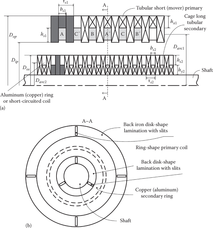
FIGURE 5.3 Tubular SLIM with cage long secondary: (a) longitudinal cross section and (b) transverse cross section.

2. Additional experience-based data

The mechanical (hereby, equal to magnetic) airgap is taken as 1.5 mm, feasible as total radial force is zero or small (when the short primary is eccentrically placed within the fix secondary).
The primary and secondary slots have to be open as the two magnetic cores are made of disk-shape silicon steel laminations, to reduce the costs of core material and fabrication.
Since the slots are open, to keep the Carter coefficient reasonable (and reduce surface core losses due to mmf harmonics and keep the power factor acceptable), the slot openings should not be larger than four airgaps in the primary and three airgaps in the secondary (this is one reason that the airgap is not too small).
As the primary coils are circular in shape, a single full pitch layer three-phase winding with (q₁ = 1 as in Figure 5.3 or q′1=2 ${q^{'}}_{1} = 2$ ) may be easily inserted in slots.
As the airgap flux/pole distributes in the primary back iron at a notably larger diameter area, the primary back-iron area radial height (h_y₁) is rather small; on the contrary, the back-iron radial height (h_y₂) in the interior secondary is larger than τ/π because the average diameter is smaller than in the airgap zone; in fact, the minimum allowable back-iron secondary interior diameter seems to be the design bottleneck.
The primary coils do not have apparent end connections, and the contact area with the slot walls is large. Consequently, the winding thermal energy transfer is good and the winding temperature is uniform; for complete fairness, we should notice that because the primary is exterior to the secondary, the average coil (turns) length is already larger than the airgap circumference so there is additional coil length (as in flat SLIMs).
Stacking the primary and secondary laminations and coils (with some local holes to exit the coil ends) thus becomes an easy task, very similar to electric transformer standard fabrication practice.
The equivalent circuit, in the absence of dynamic end and transverse edge effect (the secondary cooper rings are flowed by circular currents), is still that of Figure 5.2, and only the skin effect is present, but if inverter fed, f₂ < 10 Hz, the skin effect may be neglected. In fact, the tubular SLIM allows for smaller f₂ with copper rings, without losing much thrust density (in N/cm²) due the smaller secondary equivalent resistance for the given primary.

3. Equivalent circuit parameter expressions

For further exploration before utilization, Equation 4.36 are presented again here:

R 1 t = ρ C o π D a v c 1 I 1 r σ A l w 1 \cdot j c o r \cdot 2 \cdot w 21 = K R 1 t \cdot w 21 L 1 l t = 2 μ 0 π D a v c 1 p q 1 \cdot 2 (λ s 1 + λ d i f f 1) w 21 = K 1 l \cdot w 21 (5.47)

$\begin{array}{l} R_{1 t} = ρ_{C o} \frac{π D_{a v c 1}}{I_{1 r} σ_{A l} w_{1}} \cdot j_{c o r} \cdot 2 \cdot w_{1}^{2} = K_{R 1 t} \cdot w_{1}^{2} \\ L_{1 l t} = 2 μ_{0} \frac{π D_{a v c 1}}{p q_{1}} \cdot 2 (λ_{s 1} + λ_{d i f f 1}) w_{1}^{2} = K_{1 l} \cdot w_{1}^{2} \end{array} (5.47)$

Factor 2 accounts for the fact that two circular-shape coils mean a “pole pitch equivalent” coil.

L m t = 6 μ 0 π 2 (K w 1 \cdot w 1) 2 τ π D i p p g K c ( 1 + K s ) w 21 = K l m \cdot w 21 L' 2 l t = 2 μ 0 π D a v c 2 \cdot 12 ( K w 1 w 1 ) 2 N s 2 (λ s 2 + λ d i f f 2) = K 2 l \cdot w 21 R' 2 t = ρ A l (C o) \cdot π D a v c 2 A r i n g \cdot 12 ( K w 1 w 1 ) 2 N s 2 = K R 2 \cdot w 21 (5.47')

$\begin{array}{l} L_{m t} = \frac{6 μ_{0}}{π^{2}} {(K_{w 1} \cdot w_{1})}^{2} \frac{τπ D_{i p}}{p g K_{c} (1 + K_{s})} w_{1}^{2} = K_{l m} \cdot w_{1}^{2} \\ {L^{'}}_{2 l t} = 2 μ_{0} π D_{a v c 2} \cdot 12 \frac{{(K_{w 1} w_{1})}^{2}}{N_{s 2}} (λ_{s 2} + λ_{d i f f 2}) = K_{2 l} \cdot w_{1}^{2} \\ {R^{'}}_{2 t} = ρ_{A l (C o)} \cdot \frac{π D_{a v c 2}}{A_{r i n g}} \cdot 12 \frac{{(K_{w 1} w_{1})}^{2}}{N_{s 2}} = K_{R_{2}} \cdot w_{1}^{2} \end{array} (5.47′)$

A_ring = h_s₂ · b_s₂ · K_fill₂; K_flll₂=0.9 for solid bars and 0.6 for short-circuited copper coils.

The diameters D_avc, D_ip, D_avc₂ and the secondary slot area b_s₂ · h_s₂ are all visible in Figure 5.3.

4. Pole pitch τ_max and its design consequences

The equivalent stack length is here πD_ip, which for D_ip = 80 mm would mean 0.2512 m. The airgap was chosen as 1.5 mm (not 1 mm) to allow large enough slot openings to easily insert the coils and the secondary conductor rings in slots, though it increases the magnetization current and thus decreases the power factor. As a minimum of 40 mm solid-iron shaft is needed to form with the secondary a rigid body, it means that the secondary slot and back-iron height available would be

$h_{s 2} + h_{y 2} = \frac{D_{i p} - 2 g - 40}{2} = \frac{70 - 2 \times 1.5 - 40}{2} = 18.5 mm (5.48)$

With h_s₂ = 8 mm for the secondary slot depth, only 10.5 mm remains for the back-iron height of the secondary. Even neglecting the redistribution of flux density due to the limited length of primary (Chapter 3), and choosing a back core flux density By_2max = 1.8 T, the maximum pole pitch τ_max would be

$π D_{i p} = \frac{τ_{\max}}{π} B_{g 1 \max} = B_{y_{2} \max} π \frac{({(D_{o s} - 2 h_{s 2})}^{2} - (D_{o s} - 2 h_{s 2} - 2 h_{y 2}))}{4} (5.49)$

with D_ip = 80 mm, B_g_1max = 0.6 T (not higher here as D_ip is rather small) we may calculate the maximum pole pitch τ_max:

$τ_{\max} = \frac{1.8 \times π \times (61^{2} - 30^{2})}{0.6 \times 80 \times 4} = 83 mm (5.50)$

This is quite a reasonable value for the scope; smaller values would further decrease power factor (via lower goodness factor).

At this pole pitch, the number of slots per pole/phase q₁ = 3 to yield a slot pitch in the primary τ_s₁ = τ_max/9 = 83/9 = 9.22. The primary slot width b_s₁ = 5.5 mm < 4g = 6 mm and the primary tooth b_t₁ = 3.72 mm to secure a maximum flux density in the tooth B_t_1max ≈ B_g_1max· τ_s₁/b_t₁ = 0.6 × 9.22/3.72 = 1.48 T (thinner tooth than 3.72 mm may not be mechanically stiff enough, even after proper primary impregnation). With 8 mm deep secondary slots, we have to adopt the secondary slot pitch, which should not be for away from the primary slot pitch (to avoid important torque pulsations, noise, and vibration, as in rotary IMs).

With the secondary slot opening limited to three airgaps (4.5 mm), we may adopt a secondary tooth of b_t₁ = 4.0 mm.

Now the problem is to avoid any iteration in our preliminary design. To accomplish that, we have to choose the number of poles. Adapting a reasonably larger f_tr (for a larger airgap), f_tr = 2 N/cm², the number of poles yields

$2 p = \frac{F_{x r}}{f_{t r} \cdot π \cdot D \cdot τ_{\max}} = \frac{2500}{2 \times π \times 8 \times 8.3} \approx 6 (5.51)$

From now on, the design methodology follows the same path as for the flat SLIMs, but using the dedicated expressions of parameters.

5. The rated slip frequency f₂_r

The condition of maximum thrust per primary current is maintained. This means an about 0.707 secondary (airgap) power factor and in general smaller primary power factor, which, due to the large airgap/pole pitch ratio, is natural:

$S_{r} \cdot G_{e} = 1 (5.52)$

$G_{e} \approx \frac{ω_{1} L_{m}}{K_{l 2} R_{2}}; S K_{l 2} \sqrt{1 + (\frac{ω_{1} {L^{'}}_{2 l}}{{R^{'}}_{2}})} (5.53)$

At this moment, we may calculate ${L^{'}}_{2 l} / {R^{'}}_{2}$ as we know all the data on secondary conducting ring, but ω₁ is still missing.

From (5.53), the term $ω_{1}$ is calculated:

$\begin{array}{l} \frac{ω_{1} L_{m}}{{R^{'}}_{2}} \approx \frac{μ_{0} ω_{1 r} τ^{2} σ_{A L} \cdot h_{s 2} (1 - b_{t 2} / τ_{s 2})}{π^{2} g K_{c} (1 + K_{s})} \\ = \frac{1.256 \times 10^{- 6} \times {0.083}^{2} \times 3.25 \times 10^{7} \times 8 \times (1 - 3.75 / 9.25)}{π^{2} \times 1.5 \times 1.4 \times 1.15} \times ω_{1 r} \\ = 0.056 \times ω_{1 r} \end{array} (5.54)$

The saturation factor is taken as K_s=0.15 as the airgap is rather large and the pole pitch is not large; the Carter coefficient K_c ≈ 1.4 (it may be calculated “exactly” as in Chapter 3).

To avoid any iteration, the factor K_l₂, which accounts for L′₂_l, K_l₂ ≈ 1.1, from (5.52) to (5.54),

$S_{r} \frac{0.056 \times ω_{1}}{1.1} = 1$

Consequently,

$S_{r} ω_{1} = \frac{1.1}{0.056} = 19.64 (5.55)$

Finally

$f_{2 r} = S_{r} f_{1} = \frac{19.64}{2 π} = 3.128 Hz$

This is apparently a rather small value for LIMs, but in tubular SLIMs we may accept it because the net radial force is ideally zero so the noise and vibration at start (when f₂_r =f₁ = 3.1278 Hz) will be acceptably low.

As the speed is u_r=2 m/s, the primary frequency at rated speed f₁_r is

$f_{1 r} = f_{2 r} + \frac{u_{r}}{2 τ} = 3.1278 + \frac{2}{2 \times 0.083} = 15.176 Hz (5.56)$

It becomes evident that the primary rated frequency is only about five times the secondary (slip) frequency, so the efficiency will be below 80%, despite the fact that the core losses may be neglected by comparison with winding losses.

6. The primary phase mmf: w₁I₁_r and primary slot depth h_s₁

With sG_e = 1 and airgap flux density B_g_1max = 0.6 T from (5.23)

$\begin{array}{l} B_{g 1 \max} = \frac{μ_{0} 3 \sqrt{2} K_{w 1} \cdot w_{1} I_{1 r}}{π p g K_{c} (1 + K_{s}) 2} \\ = \frac{1.256 \times 3 \times \sqrt{2} \times 0.925 \times 10^{- 6}}{π \times 3 \times 1.5 \times 10^{- 3} \times 1.4 \times 1.15 \times 2} \times w_{1} I_{1 r} \\ = 0.1080 \times 10^{- 3} w_{1} I_{1 r} \end{array} (5.57)$

It follows that w₁I₁_r=5555 A turns/phase.

Let us verify quickly if we can obtain the required thrust (5.24):

$F_{x n} = \frac{3 π}{2 τ} I_{1 n}^{2} \frac{L_{m}}{K_{l 2}} (5.58)$

with L_m from (5.47)

$\begin{array}{l} L_{m} = \frac{6 μ_{0} K_{w 1}^{2}}{π^{2}} \frac{τπ D_{i p}}{p g K_{c} (1 + K_{s})} w_{1}^{2} \\ = \frac{6 \times 1.256 \times 10^{- 6} \times {0.925}^{2} \times 0.083 \times π \times 0.08}{π^{2} \times 3 \times 1.5 \times 10^{- 3} \times 1.4 \times 1.15} \times w_{1}^{2} \\ = 1.882 \times 10^{- 6} \times w_{1}^{2} \end{array} (5.59)$

with (5.58) in (5.57) the thrust is

$F_{x n} = \frac{3 \times 3.14}{2 \times 0.083} \times {(5555)}^{2} \times \frac{1.882 \times 10^{- 6}}{1.1} = 2925 > 2500 N (5.60)$

It is fortunate that Equation 5.60 leads to a thrust larger than required and thus the design stands (on the safe side). In case the thrust had been smaller, the whole design should have been repeated with a larger outer diameter (and pole pitch, etc.) and a larger number of poles (2p = 8, for example). The rather large specific force (2 N/cm²) “is paid for” by the large phase ampere turns w₁I₁_r, and thus larger primary copper losses, for limited stator slot depth h_s₁ (to at most 5–6 times the slot width b_s₁ = 5.5 mm, h_s₁ = 35 mm).

The phase mmf (in RMS terms) is divided into 2pq slots/phase. So the mmf per slot n_coilI₁_r is

$n_{c o i l} I_{1 r} = \frac{w_{1} I_{1 r} \times 2}{2 p q} = \frac{5555 \times 2}{2 \times 3 \times 3} = 617.2 A turns/slot (5.61)$

(Two circular coils “qualify” for a regular coil with pole pitch τ.)

So the rated current density J_cor is obtained from

$h_{s 1} = \frac{n_{c o i l} I_{1 r}}{J_{c p r} \cdot K_{f i l l} \cdot b_{s 1}} = \frac{617.2}{J_{c o r} \times 0.5 \times 5.5} = 35 mm (5.62)$

From (5.62),

$J_{c o r} = 7.833 {A/mm}^{2}$

This current density value is rather high for continuous duty cycle unless forced air cooling is applied, with a primary back-iron depth of 7 mm (it is 10.5 mm in the secondary at a much smaller diameter), mainly because of mechanical rigidity and room to assemble longitudinal bars; the outer diameter is D_op = D_ip + 2h_s₁ + 2h_y₁ = 80 + 70 + 14 + 2 = 166 mm.

We may now proceed to calculate all equivalent circuit parameters, then the number of turns/phase, wire gauge, and performance (thrust, efficiency, and power factor).

7. Number of turns per phase w₁ and equivalent circuit parameters

To calculate the number of turns/phase w₁, the equivalent parameter coefficients (5.47) should be computed first:

$\begin{array}{l} R_{1 t} = ρ_{C o} \frac{π D_{a v c 1}}{I_{1 r} w_{1}} J_{c o r} \cdot 2 w_{1}^{2} \\ = 2.3 \times 10^{- 8} \times \frac{π \times 0.116}{5555} \times 7.833 \times 10^{6} \times 2 w_{1}^{2} \\ = 2.3636 \times 10^{- 5} \times w_{1}^{2} = K_{R 1 t} \cdot w_{1}^{2} \end{array} (5.63)$

$\begin{array}{l} L_{1 l t} = \frac{2 μ_{0} π D_{a v c 1}}{p q_{1}} (λ_{s 1} + λ_{d i f f 1}) w_{1}^{2} \times 2 \\ = \frac{2 \times 1.256 \cdot 10^{- 6} \times π \times 0.116}{3 \times 3} (2.12 + 0.112) \times 2 \times w_{1}^{2} \\ = 2 \times 0.2269 \times 10^{- 6} \times w_{1}^{2} = K_{1 l t} \cdot w_{1}^{2} \end{array} (5.64)$

$λ_{s 1} \approx \frac{h_{s 2}}{3 b_{s 2}} = \frac{35}{3 \times 5.5} \approx 2.12; λ_{d i f f} \approx \frac{5 \times 1.4 \times 1.5 / 5.5}{5 + 4 \times 1.4 \times 1.5 / 5.5} = 0.112 (5.65)$

From (5.47)′,

$L_{m t} = 1.882 \times 10^{- 6} \times w_{1}^{2} = K_{m t} \cdot w_{1}^{2} (5.66)$

$\begin{array}{l} {R^{'}}_{2 t} = ρ_{A l} \cdot \frac{π D_{a v c 2}}{A_{r i n g}} \times \frac{12 \times K_{w 1}^{2}}{N_{s 2}} \times w_{1}^{2} \\ = 3.25 \times 10^{- 8} \times \frac{π \times 0 .069}{36 \times 10^{- 6}} \times \frac{12 \times {0.925}^{2}}{58} \times w_{1}^{2} \\ = 3.462 \times 10^{- 5} \times w_{1}^{2} = K_{R 2 t} \cdot w_{1}^{2} \end{array} (5.67)$

$A_{r i n g} = h_{s 2} \cdot b_{s 2} = 8 \times 4.5 = 36 (5.68)$

$N_{s 2} = N_{s 1} \cdot \frac{τ_{s 1}}{τ_{s 2}} = 6 \times 3 \times 3 \times \frac{9.22}{8.5} \approx 58 secondary slots/primary length (5.69)$

$\begin{array}{l} {L^{'}}_{2 l t} = 2 μ_{0} π D_{a v c 2} \times \frac{12 \times K_{w 1}^{2} \cdot w_{1}^{2}}{N_{s 2}} \cdot (λ_{s 2} + λ_{d i f f 2}) \\ = 2 \times 1.256 \cdot 10^{- 6} \times π \times 0.069 \times 12 \times {0.925}^{2} (\frac{0.5926 + 0.1}{58}) \times w_{1}^{2} \\ = 0.066 \times 10^{- 6} \times w_{1}^{2} = K_{2 l t} w_{1}^{2} \end{array} (5.70)$

$λ_{s 2} \approx \frac{h_{s 2}}{3 b_{s 2}} = \frac{8}{3 \times 4.5} = 0.5936; λ_{d i f f 2} = 0.1$

We are now using again the equivalent circuit (as in (5.39)) to calculate the number of turns/phase for the max voltage (120 V/phase (RMS)) and f₁_r = 15.176 Hz, f2r = sr · f1r = 3.1278 Hz:

$V_{1 r} = w_{1} \cdot (w_{1} I_{1 r}) \cdot | K_{R 1 t} + j ω_{1 r} K_{1 l t} + j \frac{K_{m t} (K_{R 2 t} / s_{r} + j ω_{1 r} K_{2 l t})}{K_{2 R t} / (s_{r} ω_{1 r}) + j (K_{m t} + K_{2 l t})} | (5.71)$

$\begin{array}{l} 120 = w_{1} \times 5555 \times 10^{- 6} | \begin{array}{l} 18.82 + j 95.3 \times 0.2269 \times 2 \\ + j 1.882 \frac{(34.62 / 0.2067 + j \times 95.3 \times 0.06)}{34.62 / 19.64 + j (1.882 + 0.06)} \end{array} | \\ 120 = w_{1} \times 5555 \times 10^{- 6} | 23.626 | + 85.97 + j 127 \end{array} (5.72)$

So, w₁ ≈ 126 turns/phase. As two coils make a pole-span equivalent coil, the number of turns/slot is

$n_{c 1} = \frac{w_{1} \times 2}{2 p q} = \frac{252}{2 \times 3 \times 3} \approx 15 turns/coil (5.73)$

So w₁_f = 135 turns/phase.

The current in the coils (all 18 coils in series) is I₁_r:

$I_{1 r} = \frac{w_{1} I_{1 r}}{w_{1}} = \frac{5555}{126} \approx 44.1 A/phase (RMS) (5.74)$

Finally, the parameters of the equivalent circuit are

$\begin{array}{l} R_{1 t} = K_{R 1 t} \cdot w_{1}^{2} = 2.3626 \times 10^{- 5} \times 126^{2} = 0.375 Ω \\ L_{1 l t} = K_{1 l t} \cdot w_{1}^{2} = 2 \times 0.2269 \times 10^{- 6} \times 126^{2} = 0.007204 H \\ L_{m t} = K_{m t} \cdot w_{1}^{2} = 1.882 \times 10^{- 6} \times 126^{2} = 0.02987 H \\ {R^{'}}_{2 t} = K_{R 2 t} \cdot w_{1}^{2} = 3.462 \times 10^{- 5} \times 126^{2} = 0.5496 Ω \\ {L^{'}}_{2 l t} = K_{2 l t} \cdot w_{1}^{2} = 0.066 \times 10^{- 6} \times 126^{2} = 0.0010478 H \end{array} (5.75)$

Now that the number of turns was reduced from 129 to 126, to maintain the rated current (for given w₁I₁_r=5555 A turns/phase (RMS)), we need to further reduce the voltage per phase to V₁_rf = V₁_r · 126/129 = 120 × 126/129 = 117.2 V/phase (RMS); so there is a further (useful) voltage reserve that will probably eliminate the necessity for overmodulation in the PWM inverter for more sinusoidal phase currents.

8. Power factor and efficiency

The power factor is evident from (5.72):

$\cos φ_{1} = \frac{Re (Z e)}{| \underline{Z e} |} = \frac{109.596}{167.00} \approx 0.6 (5.76)$

To calculate the efficiency, we first have to determine the electromagnetic power P_elm.

$P_{e l m} = F_{x r} \cdot U_{s}; U_{s} = 2 τ f_{1 r} = 2 \times 0.083 \times 15.176 = 2.5192 m/s (5.77)$

But

$\begin{array}{l} P_{e l m} = P_{1} - 3 R_{1} I_{1 r}^{2} = 3 V_{1 r} I_{1 r} \cos φ_{1} - 3 R_{1} I_{1 r}^{2} \\ = 3 \times 117.2 \times 44.1 \times 0.6 - 3 \times 0.375 \times {44.1}^{2} = 7115 W \end{array} (5.78)$

So the thrust is in fact

$F_{x} = 7115 / 2.5192 = 2824 N (5.79)$

The efficiency is in fact

$η_{1} = \frac{F_{x} U_{r}}{P_{1}} = \frac{2824 \times 2}{9303} = 0.607 (5.80)$

Discussion

The required 2.5 kN thrust was surpassed in the preliminary design to 2.824 kN at a specific force of almost 2.4 N/cm² of primary; this is a rather large value for an LIM.
The power factor is rather good for LIMs (cos φ₁ = 0.60); the price to pay for high force density is the lower efficiency, which implies forced air cooling, at least for the primary.
The forecasted 0.37 of η₁ cos φ₁ product is a fairly good LIM performance for 2 m/s
For given travel length and duty cycle, the temperature of the fix secondary may be assessed by fairly simple equivalent thermal circuit models [5].
For better efficiency at the price of a heavier primary and secondary, the overall D_op and primary bore D_ip diameters have to be increased and the design routine has to be repeated (a simple MATLAB^®-code would take only a few seconds to do it).

9. Note on optimization design

For low-speed (negligible dynamic end effect) SLIMs with ladder secondary, the optimization design is very similar to that of rotary IMs [6]. Only parameter and performance expressions and the objective function should be adapted for the scope. For medium- and high-speed (transportation) LIMs, the optimization design will be approached in some detail, as there are more notable differences with respect to the case of rotary IMs (Chapter 6).

5.4 Summary

By low-speed LIMs it is meant low (negligible end effect) LIMs ((γ₂_rτ)⁻¹ < 2p/10, Chapter 3); speeds up to 5–6 m/s in adequate design LIMs may fall into this category.
To raise the efficiency × power factor product from 0.2–0.25 to 0.36, only cage-secondary SLIMs with 1–1.5 mm airgaps are considered.
Only for medium- and high-speed LIMs (Chapter 6), the aluminum-iron secondary will be investigated, in long travel of hundreds of meters to tens and hundreds of kilometers.
The design airgap flux density in ladder secondary, for 1–1.5 mm airgap, low speed (up to 5–6 m/s) should be in the range of 0.6–0.7 T to yield reasonable thrust density (1–2 N/cm²).
In flat SLIMs with cage secondary, the normal (attraction) force is even more than 20 times the thrust and is recommended to be used for the “almost” entire mover (plus load) suspension to relieve the linear bearing of too high mechanical stresses.
In tubular SLIMs, the net normal force is ideally zero, and in up to 1–2 m long travels (even longer) it may be the preferred solution.
For the design of flat (or tubular) low-speed SLIMs, the equivalent circuit of IMs is used with dedicated expressions for the parameters: R₁ L₁_l, L_m, R′₂, L′₂_l; as both cores are laminated, and the secondary frequency is lower than 10 Hz, the skin effect in the secondary conductor rings in slots is moderate, so that only magnetic saturation has some but limited influence (the airgap/pole pitch ratio is not very small, as in rotary IMs).
By design we mean here dimensioning (sizing), that is, to find a suitable geometry for a SLIM of given specifications.
The key design concept used here is the maximum thrust per primary mmf (current), which leads to S_rG_e=1; this represents a practical compromise between acceptable efficiency and primary weight/thrust.
The slip (secondary) frequency for rated thrust is chosen here (for the case studies in this chapter f₂_r=4 Hz, respectively, 3 Hz for the flat, respectively tubular, rather medium thrust 500 N (2500 N) and 3(2) m/s).
With a low (0.88 N/cm²) specific thrust, 0.707 power factor and 0.711 efficiency were obtained for the flat ladder-secondary SLIM for 615N at 3 m/s, with a short (mover) primary of about 36 kg; this may be considered competitive performance in some applications where ruggedness and low initial costs are prevalent.
On the contrary, for the tubular ladder-secondary SLIM at 2.4 N/cm², cos φ=0.6, at 2824 N at 3 m/s for an 0.166 m outer primary diameter (0.08 m inner primary diameter), 0.5 m long primary (about 66 kg short primary weight).
The tubular SLIMs with cage secondary and disk-shape laminations in both primary and secondary cores lead to negligible core losses in most low-speed designs and represent an easy manufacturable topology.
Flat SLIMs with ladder long secondary and short primary are already commercial in some machine-tool table, etc., applications.
Even for low-speed (say, at 5–6 m/s) SLIM designs, dynamic end effect may be accepted by choosing higher goodness factor topologies (higher frequency and pole pitch) when both conventional performance and the deteriorating dynamic end effect rise; but the compromise at optimum goodness factor (Chapter 4)—zero end effect force at zero slip— may end up in better performance; this case is implicit, however, in medium- or high-speed SLIMs design, to be treated in Chapter 6.
Optimization analytical design of low-speed (negligible dynamic end effect) SLIMs is too similar to that of rotary IMs treated here [see Ref. 6].
2(3)D FEM-based direct geometrical design after optimization analytical design should follow, but this is beyond our scope here.

References

1. I. Boldea and S.A. Nasar, Simulation of High Speed LIM End Effects is Low Speed Tests, Proc. IEEE, 121(9), 1974, 961–964.

2. I. Gieras, Linear Induction Drives, Clarendon Press, Oxford, U.K., 1994.

3. I. Boldea and S.A. Nasar, Linear Electric Actuators and Generators, Cambridge University Press, Cambridge, U.K., 1997.

4. I. Boldea and S.A. Nasar, Linear Motion Electromagnetic Devices, Taylor & Francis, New York, 2001.

5. I. Boldea and S.A. Nasar, Induction Machine Design Handbook, 2nd edn., CRC Press, Taylor & Francis Group, New York, 2010.

6. I. Boldea and L. Tutelea, Electric Machines: Steady State Transients and Design with Matlab, CRC Press, Taylor & Francis, New York, 2009.

..................Content has been hidden....................

You can't read the all page of ebook, please click here login for view all page.

Table of Contents for
Chapter 5 Design of Flat and Tubular Low-Speed LIMs

5 Design of Flat and Tubular Low-Speed LIMs

5.1 Introduction

5.2 Flat SLIM with Ladder Long Secondary and Short Primary

5.3 Tubular SLIM with Cage Secondary

5.4 Summary

References

Table of Contents for Chapter 5 Design of Flat and Tubular Low-Speed LIMs

Create new playlist

Sign In

Sign Up

5 Design of Flat and Tubular Low-Speed LIMs

5.1 Introduction

5.2 Flat SLIM with Ladder Long Secondary and Short Primary

5.3 Tubular SLIM with Cage Secondary

5.4 Summary

References

Table of Contents for
Chapter 5 Design of Flat and Tubular Low-Speed LIMs