Chapter 17 Resonant Linear Oscillatory Single-Phase PM Motors/Generators

Search in book...
Toggle Font Controls
Create new playlist

Name your new playlist

Playlist description (optional)
Sign In

Email address

Password

Forgot Password?

or

Continue with Facebook

Continue with Google
Sign Up

Full Name

Email address

Confirm Email Address

Password

or

Continue with Facebook

Continue with Google

Fixed frequency linear motion applications [1] such as compressors, pumps, vibrators, as well as speakers/microphones use linear oscillatory single-phase PM motors (LOMs), while short-stroke (up to 20 mm in general) applications use linear single-phase PM generators (LOGs) such as Stirling engines or other linear piston engines due to

Elimination of rotary to linear motion mechanical transmission
Simplicity and ruggedness of their topology
Rather high efficiency and high force density, especially with mechanical springs and operation at resonance frequency (mechanical eigenfrequency = electrical frequency)
Simplicity (single-phase PWM converter) for close-loop control

Note: Other linear generators with larger stroke (20 mm and more) have been investigated in 2(3) phase configurations in previous chapters. Here only the single-phase ones are treated.

The LOMs (LOGs) may be classified into three main categories:

With coil mover
With PM mover
With iron mover

Flat and tubular, single-phase PM topologies are feasible, but the tubular ones are favored, as the blessing of circularity leads to better volume usage and better heat transmission. As expected, each category exhibits a plethora of different topologies, with a few being actually practical.

This chapter will deal with the tubular coil-mover LOM (LOG) both for large power (25 kW— say for series hybrid electric vehicles) and for very small power microphones and vibrators of mobile phones.

Then the PM-mover topology in its tubular shape will be treated in both single- and multiple-pole (and stator coil) variants for refrigerator-like compressors. In addition, the flat PM-mover LOM (LOG) in reversal flux configurations with PM flux concentration will be investigated due to its high-performance potential.

Finally, a tubular and a flat iron-mover LOM (LOG) will be covered, from topology through modeling, FEM-analysis dynamics, control, and optimal design with case studies.

17.2 Coil-Mover LOMs (LOGs)

Single-coil (or homopolar)-mover LOMs (Figure 17.1a) are typical for strokes up to 100 mm for high-rated forces: hundreds of Newtons to kN at frequencies below 6–70 Hz and for much lower forces, in the sub-mm range, for microspeakers in mobile phones, etc.

Images

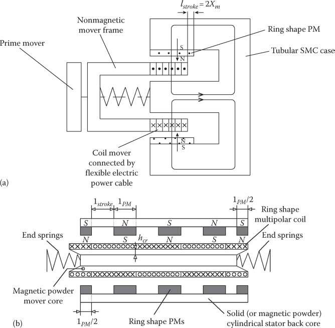
FIGURE 17.1 Coil-mover LOM(G), (a) single-coil–single PM, (b) multiple-coil-multiple PM.

The multiple-coil topology (Figure 17.1b) should be preferable when the weight of the core (and total weight) is critical and thus the multi-PM poles lead to lower PM core flux. The flexible electric power cable (or even slip rings and brushes) to transmit or collect the electric input (output) power is a demerit of the coil-mover solution; however, the mass M of the mover is reduced, so that the mechanical spring constant K, for the given resonance frequency, is smaller; the cost of the spring is reduced:

2 π f_{m} = \sqrt{\frac{K}{M}} (17.1)

$2 π f_{m} = \sqrt{\frac{K}{M}} (17.1)$

In Figure 17.1, the coil length is longer than the PM length by the stroke length, l_stroke:

\begin{matrix} l_{s t o r k e} \approx 2 X_{m} & X_{m} : Motion amplitude \end{matrix} (17.2)

$\begin{matrix} l_{s t o r k e} \approx 2 X_{m} & X_{m} : Motion amplitude \end{matrix} (17.2)$

This leads to lower PM weight but to more mover weight and copper losses. The shorter coil– longer PM by (l_stroke) combination (Figure 17.1a) may also be adopted for the multiple-coil topology (Figure 17.1b).

But larger PMs mean more costs and thicker stator core and weight.

Depending on the key constraints of application, one or the other option is used in the design.

Images

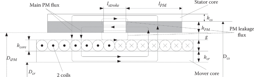
FIGURE 17.2 Two-coil mover two-PM pole stator LOM (G).

The air coil(s) leads to smaller inductance and thus larger power factor, but it also implies lower thrust density; the fragility of the coil mover, which has to be enforced with a nonmagnetic frame (siluminum), may also be a problem as the electromagnetic force is exerted directly on the conductors of the coil(s).

In an effort to reconcile these conflicting requirements, for large power devices (kW range and more), a two or more pole topology is selected; this time the inner magnetic core may be attached to the mover to reinforce it mechanically, in spite of its additional mover weight (Figure 17.2).

Additional axially magnetized PMs may be added to produce more flux density in the coils, but also to reduce outer core flux (and radial thickness).

The dual (multiple)-coil-mover LOM may also be manufactured for smaller diameter and larger axial length geometry.

As the average PM airgap flux density is around 0.5 × B_r at best, LOM(G), due to the air-core coils’ mild magnetic saturation in the cores, can be kept under control, without excessive core volume, but the thrust density remains moderate.

17.2.1 Four-Coil-Mover LOM: Modeling and Design by Example

Let us consider the configuration in Figure 17.2 (but with four PMs and four coils) and develop an analytical model for it, and then use this model for preliminary electromagnetic design as a generator for an electrical output of 20 kW, 220 V_RMS, f₁ = 60 Hz, stroke length l_stroke = 30 mm, and for harmonic (sinusoidal) motion: x = l_stroke/2sin(2πf₁t).

To limit the space required for presentation, we will first define the objectives and then proceed, in parallel, with the modeling and the numerical example: airgap PM flux density, airgap diameter and PM sizing, emf, thrust, inductance, resistance and core losses, core sizing and core loss, voltage equation and phasor diagram, number of turns (total), efficiency, power factor and its compensation by a capacitor, mover weight, and mechanical spring rigidity constant K.

17.2.1.1 Airgap: PM Flux Density

Making use of the Ampere law, while accounting for the axial PM and for the flux fringing and for magnetic saturation by equivalent coefficients, K_aPM < 0.3, K_fringe < 0.2, K_sat < 0.1 (large total airgap), the airgap PM flux density B_gPM is

B_{g P M} = \frac{B_{r} h_{P M} μ_{r e c} (1 + K_{a P M})}{h_{P M} + (g + l_{c o i l}) μ_{r e c} (1 + K_{f r i n g e}) (1 + K_{s a t})} (17.3)

$B_{g P M} = \frac{B_{r} h_{P M} μ_{r e c} (1 + K_{a P M})}{h_{P M} + (g + l_{c o i l}) μ_{r e c} (1 + K_{f r i n g e}) (1 + K_{s a t})} (17.3)$

In Equation 17.3, the curvature of the tubular structure is neglected as the thrust, power, and airgap diameter are notable.

The optimum h_PM/g ratio is chosen for the simplified expression (17.3) such that h_PMμ_rec/g ≈ 1; a more elaborated optimization design should consider the thrust/volume and thrust/copper losses, but the results will not be far from this approximation.

Let us consider this condition met and, by FEM, K_aPM = 0.20, K_sat = 0.1, K_fringe = 0.1. With B_r = 1.2 T (μ_rec = 1.05 p.u.), from (17.3)

B_{g P M} \approx \frac{B r}{2} = 0.6 T (17.4)

$B_{g P M} \approx \frac{B r}{2} = 0.6 T (17.4)$

17.2.1.1.1 Airgap Diameter D_iPM and PM Length l_PM

To size the LOG, the thrust has to be known by assuming an efficiency η_n ≈ 0.93 and calculating the average speed U_av:

\begin{array}{l} U_{a v} = 2 l_{s t r o k e} f_{1} = 2 \cdot 0.03 \cdot 60 = 3.6 m/s \\ F_{x a v} = \frac{P_{n}}{U_{a v} η_{n}} = \frac{2 \cdot 1^{3}}{3.6 \cdot 0.93} = 5973.7 N \end{array} (17.5)

$\begin{array}{l} U_{a v} = 2 l_{s t r o k e} f_{1} = 2 \cdot 0.03 \cdot 60 = 3.6 m/s \\ F_{x a v} = \frac{P_{n}}{U_{a v} η_{n}} = \frac{2 \cdot 1^{3}}{3.6 \cdot 0.93} = 5973.7 N \end{array} (17.5)$

A moderate flux density f_xπ = 2 N/cm² is adopted. Consequently, the total active PM area A_PM is

A_{P M} = \frac{F_{x a v}}{f_{x r}} = \frac{5973.7}{2 \cdot 310^{4}} = 0.2986 m^{2} (17.6)

$A_{P M} = \frac{F_{x a v}}{f_{x r}} = \frac{5973.7}{2 \cdot 310^{4}} = 0.2986 m^{2} (17.6)$

Now the problem is to discriminate between PM length and airgap diameter D_iPM. It is evident that the PM pole length (l_PM) should be longer than stroke length, in order to limit the additional copper losses in the inactive core length (2pl_stroke); 2p—coils (PMs); in our case p = 2.

Let us consider l_PM=2l_stroke = 2 · 0.03 = 0.06 m. For 4 active poles, the airgap diameter D_iPM is approximately

D_{i P M} \approx \frac{A_{P M}}{2 p l_{P M} π} = \frac{0.2986}{4 \cdot 6 \cdot 10^{- 2} \cdot π} = 0.396 m (17.7)

$D_{i P M} \approx \frac{A_{P M}}{2 p l_{P M} π} = \frac{0.2986}{4 \cdot 6 \cdot 10^{- 2} \cdot π} = 0.396 m (17.7)$

But the average thrust (Lorenz force) F_xav is

F_{x a v} \approx B_{g P M} \frac{l_{P M}}{l_{P M} + l_{s t r o k e}} \cdot π \cdot D_{a v c} \cdot 2 p; n_{c} \cdot I_{a v}; I_{n} \sqrt{2} \cdot \frac{2}{π} (17.8)

$F_{x a v} \approx B_{g P M} \frac{l_{P M}}{l_{P M} + l_{s t r o k e}} \cdot π \cdot D_{a v c} \cdot 2 p; n_{c} \cdot I_{a v}; I_{n} \sqrt{2} \cdot \frac{2}{π} (17.8)$

n_c is the turns per coil (there are 2p coils) and each coil is l_PM + l_stroke in length. But for a given current density j_con = 6 A/m² and coil filling factor K_fill = 0.8 (the coil may be made of multiple thin copper foils),

\frac{n_{c} I_{a v}}{l_{P M} + l_{s t r o k e}} = j_{c o n} \cdot h_{c o i l} \cdot k_{f i l l} \cdot n_{c} \cdot I_{a v} = 0.09 \cdot 6 \cdot 10^{6} \cdot h_{c o i l} \cdot 0.8 (17.9)

$\frac{n_{c} I_{a v}}{l_{P M} + l_{s t r o k e}} = j_{c o n} \cdot h_{c o i l} \cdot k_{f i l l} \cdot n_{c} \cdot I_{a v} = 0.09 \cdot 6 \cdot 10^{6} \cdot h_{c o i l} \cdot 0.8 (17.9)$

h_{c o i l} = \frac{n_{c} \cdot I_{a v}}{0.432 \cdot 10^{6}} (17.10)

$h_{c o i l} = \frac{n_{c} \cdot I_{a v}}{0.432 \cdot 10^{6}} (17.10)$

Also,

D_{a v c} \approx D_{i P M} - g - h_{c o i l}; g = 1.5 mm (17.11)

$D_{a v c} \approx D_{i P M} - g - h_{c o i l}; g = 1.5 mm (17.11)$

From (17.8) through (17.11), we may calculate simultaneously h_coil ≈ (h_PM+ g)/μ_rec and n_cI_av: π_cI_av ≈ 3017 A turns/coil and h_coil = 7.0 · 10⁻³ m.

So the PM height h_PM = h_coil · μ_rec + g = 7 · 1.05 + 1.5 = 8.85 mm = 8.85 · 10⁻³ m; D_avc=D_iPM−(g + h_coil) = 0.396 − (1.5 + 7.0) · 10⁻³ ≈ 0.386 m.

The total resistance R_s is

R_{s} = 2 p \cdot ρ_{c o} \frac{π D_{a v c} n_{c}^{2} j_{c o n}}{n_{c} I_{a v}} = \frac{4 \cdot 2.0 \cdot 10^{- 8} \cdot π \cdot 0.386 \cdot 6 \cdot 10^{6} \cdot n_{c}^{2}}{3017} = 2.603 \cdot 10^{- 4} n_{c}^{2} (17.12)

$R_{s} = 2 p \cdot ρ_{c o} \frac{π D_{a v c} n_{c}^{2} j_{c o n}}{n_{c} I_{a v}} = \frac{4 \cdot 2.0 \cdot 10^{- 8} \cdot π \cdot 0.386 \cdot 6 \cdot 10^{6} \cdot n_{c}^{2}}{3017} = 2.603 \cdot 10^{- 4} n_{c}^{2} (17.12)$

So the copper losses p_con are

p_{c o n} \approx R_{s} I_{a v}^{2} = 2.60 \cdot 10^{- 4} \cdot 3017^{2} = 1755 W (17.13)

$p_{c o n} \approx R_{s} I_{a v}^{2} = 2.60 \cdot 10^{- 4} \cdot 3017^{2} = 1755 W (17.13)$

With iron and mechanical losses neglected, the copper losses would lead to an “ideal” efficiency of 0.92. As this is not far away from the assigned value of 0.93, and we are dealing here with a preliminary design, the obtained geometry holds; otherwise, the design should be redone from (17.5) with a lower (0.9) value of assigned efficiency.

17.2.1.2 Inductance

The inductance comprises essentially only the airgap component:

\begin{array}{l} L_{s} \approx \frac{1}{8} 2 p μ_{0} n_{c}^{2} π D_{a v c} \frac{(l_{P M} + l_{s t r o k e})}{\frac{h_{P M}}{μ_{r e c}} + g + h_{c o i l}} = \frac{1}{8} \cdot 4 \cdot 1.256 \cdot 10^{- 6} \cdot π \cdot 0.386 \cdot \frac{0.09}{(\frac{8.85}{1.05} + 1.5 + 7.0) \cdot 10^{- 3}} n_{c}^{2} \\ = 4.06 \cdot 10^{- 6} n_{c}^{2} \end{array} (17.14)

$\begin{array}{l} L_{s} \approx \frac{1}{8} 2 p μ_{0} n_{c}^{2} π D_{a v c} \frac{(l_{P M} + l_{s t r o k e})}{\frac{h_{P M}}{μ_{r e c}} + g + h_{c o i l}} = \frac{1}{8} \cdot 4 \cdot 1.256 \cdot 10^{- 6} \cdot π \cdot 0.386 \cdot \frac{0.09}{(\frac{8.85}{1.05} + 1.5 + 7.0) \cdot 10^{- 3}} n_{c}^{2} \\ = 4.06 \cdot 10^{- 6} n_{c}^{2} \end{array} (17.14)$

The emf (E)

E (t) = B_{g P M} \cdot U (t) \cdot π \cdot D_{a v c} \cdot 2 p \cdot n_{c} \frac{l_{P M}}{l_{P M} + l_{s t r o k e}} (17.15)

$E (t) = B_{g P M} \cdot U (t) \cdot π \cdot D_{a v c} \cdot 2 p \cdot n_{c} \frac{l_{P M}}{l_{P M} + l_{s t r o k e}} (17.15)$

The speed is

U (t) = ω_{1} x_{m} \cos ω_{1} t = 2 π \cdot 50 \cdot 0.015 \cdot \cos ω_{1} t = 4.71 \cdot \cos ω_{1} t (17.16)

$U (t) = ω_{1} x_{m} \cos ω_{1} t = 2 π \cdot 50 \cdot 0.015 \cdot \cos ω_{1} t = 4.71 \cdot \cos ω_{1} t (17.16)$

E (t) = 0.6 \cdot 4.71 \cdot π \cdot 0.386 \cdot 4 \cdot \frac{0.06}{0.09} \cdot n_{c} \cdot \cos ω_{1} t = 9.134 \cdot n_{c} \cdot \cos ω_{1} t (17.17)

$E (t) = 0.6 \cdot 4.71 \cdot π \cdot 0.386 \cdot 4 \cdot \frac{0.06}{0.09} \cdot n_{c} \cdot \cos ω_{1} t = 9.134 \cdot n_{c} \cdot \cos ω_{1} t (17.17)$

In (17.15), a PM flux linkage in the coil linear variation with position is supposed; consequently, the harmonic motion leads to a sinusoidal emf. In reality, at the ends of PMs, both the emf and thrust are somewhat reduced; these effects have to be calculated by 2D FEM and accounted for by fudge factors in the force and emf expressions.

17.2.1.3 Core Sizing and Core Losses

As the PM airgap flux density is B_gPM = 0.6 T, the peak “armature reaction” is

B_{a g p e a k} \approx B_{g P M} \frac{ω_{1} L_{s} I_{R M S}}{E_{1 R M S}} = \frac{.6 \cdot 100 \cdot π \cdot 4.096 \cdot 10^{- 6} n_{c}^{2} I_{R M S}}{(9.130 \cdot n_{c} / \sqrt{2})} \approx 0.395 T (17.18)

$B_{a g p e a k} \approx B_{g P M} \frac{ω_{1} L_{s} I_{R M S}}{E_{1 R M S}} = \frac{.6 \cdot 100 \cdot π \cdot 4.096 \cdot 10^{- 6} n_{c}^{2} I_{R M S}}{(9.130 \cdot n_{c} / \sqrt{2})} \approx 0.395 T (17.18)$

The average PM flux in the cores is given, however, by the B_gPM, as magnetic saturation is kept under control with B_cs=B_cm ≈ 1.5 T. For 2p = 4 PM poles not 1/2 but approximately 2/3 of PM pole flux travels the coils axially.

The stator outer core depth h_cs is

h_{c s} \approx \frac{2}{3} \frac{B_{g P M} \cdot l_{P M} \cdot π (D_{i P M} + 2 h_{P M} + h_{P M})}{B_{c s} π (D_{i P M} + 2 h_{P M} + (h_{c s}))} (17.19)

$h_{c s} \approx \frac{2}{3} \frac{B_{g P M} \cdot l_{P M} \cdot π (D_{i P M} + 2 h_{P M} + h_{P M})}{B_{c s} π (D_{i P M} + 2 h_{P M} + (h_{c s}))} (17.19)$

From (17.19), with B_gPM = 0.6T, l_PM = 0.06 m, D_iPM = 0.396 mm, mm, h_cs ≈ 16 mm.

In a similar way, the thickness of the mover core is h_cm = 18 mm.

Now the iron weight—for both stator and mover—is

\begin{array}{l} G_{i r o n s m} = 2 p (l_{P M} + l_{s t r o k e}) \cdot π (D_{i P M} + 2 h_{P M} + h_{c s}) \cdot h_{c s} \cdot γ_{i r o n} \\ = 4 \cdot 0.09 \cdot π (0.396 + 2 \cdot 0.00855 + 0.016) \cdot 0.016 \cdot 7200 \\ = 55 kg \end{array} (17.20)

$\begin{array}{l} G_{i r o n s m} = 2 p (l_{P M} + l_{s t r o k e}) \cdot π (D_{i P M} + 2 h_{P M} + h_{c s}) \cdot h_{c s} \cdot γ_{i r o n} \\ = 4 \cdot 0.09 \cdot π (0.396 + 2 \cdot 0.00855 + 0.016) \cdot 0.016 \cdot 7200 \\ = 55 kg \end{array} (17.20)$

\begin{array}{l} G_{i r o n s} = 2 p (l_{P M} + l_{s t r o k e}) \cdot π (D_{i P M} - 2 (g + h_{c o i l}) - h_{c m}) \cdot h_{c m} \cdot γ_{i r o n} \\ = 4 \cdot 0.09 \cdot π (0.396 + 2 (1.5 + 7.0) \cdot 10^{- 3} - 0.018) \cdot 0.018 \cdot 7200 \\ = 52.84 kg \end{array} (17.21)

$\begin{array}{l} G_{i r o n s} = 2 p (l_{P M} + l_{s t r o k e}) \cdot π (D_{i P M} - 2 (g + h_{c o i l}) - h_{c m}) \cdot h_{c m} \cdot γ_{i r o n} \\ = 4 \cdot 0.09 \cdot π (0.396 + 2 (1.5 + 7.0) \cdot 10^{- 3} - 0.018) \cdot 0.018 \cdot 7200 \\ = 52.84 kg \end{array} (17.21)$

Note: the mover iron weight seems large and may be “moved” to an interior stator, by splitting the airgap in two and making the coil-mover structure of nonmagnetic (siluminum) materials; its mechanical ruggedness has then to be considered carefully.

With SMC cores, the P_iron at 1.5 T/50 Hz may be considered to be 4 W/kg, so the total core losses may be as high as 4 W/kg · 110 kg = 440 W. This is nontrivial and should be considered in efficiency calculations and in the thermal design. A lower core loss material would be beneficial, provided its cost is affordable for the application.

17.2.1.4 The Phasor Diagram

The coil-mover LOM(G) is in fact a single-phase synchronous machine where the sinusoidal emf is produced by the harmonic motion, while the PM flux linkage per coil varies linearly with mover position; the inductance is independent of mover position as the machine exhibits air coils.

Under steady state, at resonance, $ω_{1} = ω_{m} = 2 π \sqrt{k / M}$ $ω_{1} = ω_{m} = 2 π \sqrt{k / M}$ , the mechanical spring “moves” the mover back and forth, with small mechanical losses, while the electromagnetic (Lorenz) force produces electromagnetic power for the load.

The decreases in force (and emf) coefficients Ke(x), (F_x=K_ei), toward the ends of stroke, are in general less than 10%, and thus a sinusoidal emf may be used for the preliminary design. Also, the cogging force is practically zero. Consequently, the standard phasor diagram may be used, based on steady-state voltage equation in complex variable terms (Figure 17.3)

Images

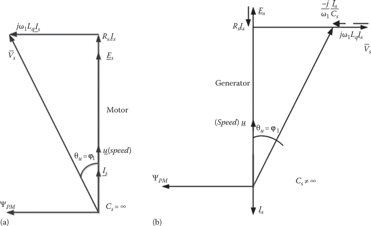
FIGURE 17.3 Coil-mover LOM(G); the phasor diagram for resonance conditions (a) motoring, (b) generating.

\underline{V_{s}} = R_{s} \underline{I_{s}} + j ω_{1} L_{s} \underline{I_{s}} - j \frac{1}{ω_{1} C_{s}} \underline{I_{s}} + K_{e} \underline{U} (17.22)

$\underline{V_{s}} = R_{s} \underline{I_{s}} + j ω_{1} L_{s} \underline{I_{s}} - j \frac{1}{ω_{1} C_{s}} \underline{I_{s}} + K_{e} \underline{U} (17.22)$

U is speed phasor; ${\underline{E}}_{\underline{s}} = K_{e} \underline{U}$ ${\underline{E}}_{\underline{s}} = K_{e} \underline{U}$

For resonance conditions ω₁ = ω_m and the current is in phase with emf (and speed), to produce maximum power/current. In this case, however, the power factor is lagging (for motoring) and the voltage regulation is notable for generating.

A series capacitor (C_s) may be used to compensate (or overcompensate) the inductance L_s, to extract more power for a given machine at given output voltage in generating and provide for stability in autonomous operation, as shown later in this chapter when stability and control aspects are treated. The series capacitor C_s may be used in the motoring also to only partially compensate for the inductance L_s and thus improve the power factor and increase starting current for faster self-synchronization at direct connection to the power grid; care must be exercised in this case to avoid PM demagnetization during C_s-assisted direct starting; ultimately, C_s may be shorted during direct starting.

17.2.1.5 The Number of Turns per Coil n_c

From the phasor diagram

\begin{matrix} {(E_{s} - R_{s} I_{s})}^{2} + ω_{1}^{2} L_{s}^{2} I_{s}^{2} = V_{s}^{2}; & I_{s} = I_{R M S} = I_{a v} \cdot (\frac{π}{2 \sqrt{2}}) \end{matrix} (17.23)

$\begin{matrix} {(E_{s} - R_{s} I_{s})}^{2} + ω_{1}^{2} L_{s}^{2} I_{s}^{2} = V_{s}^{2}; & I_{s} = I_{R M S} = I_{a v} \cdot (\frac{π}{2 \sqrt{2}}) \end{matrix} (17.23)$

Making use of already calculated parameters,

\begin{array}{l} \begin{matrix} E_{s} = 2.2835 \cdot \frac{n_{c}}{\sqrt{2}}; & R_{s} I_{s} = 2.603 \cdot 10^{- 4} n_{c} (n_{c} I_{s}) \end{matrix} \\ \begin{matrix} ω_{1} L_{s} I_{s} = 100 \cdot π \cdot 4.046 \cdot 10^{- 6} n_{c} (n_{c} I_{s}), & V_{S} = 200 V (R M S) \end{matrix} \end{array}

$\begin{array}{l} \begin{matrix} E_{s} = 2.2835 \cdot \frac{n_{c}}{\sqrt{2}}; & R_{s} I_{s} = 2.603 \cdot 10^{- 4} n_{c} (n_{c} I_{s}) \end{matrix} \\ \begin{matrix} ω_{1} L_{s} I_{s} = 100 \cdot π \cdot 4.046 \cdot 10^{- 6} n_{c} (n_{c} I_{s}), & V_{S} = 200 V (R M S) \end{matrix} \end{array}$

The number of turns/coil n_c (there are four coils in series) is

n_{c} \frac{220}{\sqrt{{5.8952}^{2} + {4.235}^{2}}} = \frac{220}{7.2587} \approx 31 turns/coil (17.24)

$n_{c} \frac{220}{\sqrt{{5.8952}^{2} + {4.235}^{2}}} = \frac{220}{7.2587} \approx 31 turns/coil (17.24)$

So the current I₁ (RMS) is

I_{1 R M S} = \frac{n_{c} I_{a v}}{n_{c}} \cdot \frac{π}{2 \sqrt{2}} = \frac{3017}{31} \cdot \frac{π}{2 \sqrt{2}} = 108.36 A (17.25)

$I_{1 R M S} = \frac{n_{c} I_{a v}}{n_{c}} \cdot \frac{π}{2 \sqrt{2}} = \frac{3017}{31} \cdot \frac{π}{2 \sqrt{2}} = 108.36 A (17.25)$

The power factor cos φ is [from (17.26)]

\cos φ = \frac{5.8952}{7.2587} = 0.812 (17.26)

$\cos φ = \frac{5.8952}{7.2587} = 0.812 (17.26)$

For motoring, the power factor should have been better, but to operate at the same voltage, (without any series capacitor), the number of turns would have been different.

Including the core losses, the machine efficiency would be about 1.6% smaller (90.4%). It has to be borne in mind that the designed LOG is a rather low-speed U_av ≈ 3.6 m/s machine, which explains the moderate efficiency, but the elimination of mechanical transmission and the increased reliability might pay off.

The copper weight in the mover can be easily calculated and, after admitting additional mover mass for framing and from the prime mover (or load machine: compressor for motoring), the mechanical spring rigidity K may be calculated, at resonance frequency.

In an attempt to reduce copper losses and eliminate the electric power flexible cable, the PMs (longer than coils) may be placed on the mover but then core weights will be larger.

Note: Though we may follow here other aspects of LOM(LOG), we will exercise them over other topologies, to spread more evenly the new knowledge over this chapter.

17.2.2 Integrated Microspeakers and Receivers

Microspeakers and receivers are required for advanced mobile phones that integrate laptop PC functions, web searching, MP3 song players, etc. [2–4].

High-quality sound, broader frequency range, and reduced size and costs are paramount for microspeakers and receivers. Harmonic distortion affects the quality of sound and is defined by the ratio between the sum of sound power of higher harmonics to the power of fundamental frequency.

Harmonic distortion is produced by the diaphragm asymmetry, input source voltage harmonics, and uneven magnetic field distribution. The latter also influences the sound pressure level (SPL). These are all related to the microspeaker/receiver design.

But for an acoustical analysis, the sound power radiated, which vibrates in a mean rms surface with speed of $({\dot{x}}^{2} (f))$ $({\dot{x}}^{2} (f))$ , is

W_{r a d} (f) = ρ c S_{r a d} σ_{r a d} (f) < {\dot{x}}^{2} (f) > . [W] (17.27)

$W_{r a d} (f) = ρ c S_{r a d} σ_{r a d} (f) < {\dot{x}}^{2} (f) > . [W] (17.27)$

where

ρ is air density

c is the sound speed in air

f is the radiation frequency S_rad is the diaphragm area

σ_rad is the radiation efficiency

For a monopole source type diaphragm, [5]

σ_{r a d} (f) = \frac{K^{2} a^{2}}{1 + K^{2} a^{2}} (17.28)

$σ_{r a d} (f) = \frac{K^{2} a^{2}}{1 + K^{2} a^{2}} (17.28)$

K = 2πf/c is the wave number, and a is the diaphragm radius. The sound pressure level (SPL) at distance d from the source L_p(d) is

L_{p} (d) = L_{w} - 20 \log (\frac{d}{d_{0}}) - 8; [dB] (17.29)

$L_{p} (d) = L_{w} - 20 \log (\frac{d}{d_{0}}) - 8; [dB] (17.29)$

L_w is the sound power level, d₀ = 1 m:

L_{w} (d) = 10 \log (\frac{W_{r a d}}{10^{- 12}}); [dB] (17.30)

$L_{w} (d) = 10 \log (\frac{W_{r a d}}{10^{- 12}}); [dB] (17.30)$

Finally, the total harmonic distortion (THD) in % is [5]

TWD = \frac{Sum † of † power † in † harmonics (ν \geq 2)}{Total † power} (17.31)

$TWD = \frac{Sum † of † power † in † harmonics (ν \geq 2)}{Total † power} (17.31)$

The microspeaker and the dynamic receiver in the cellular phones may be separate units, but, to reduce space, the integration of the two in one piece seems a practical solution (Figure 17.4) [4]. Consequently, only the integrated solution is detailed here.

The two-coil motors are both placed (Figure 17.4c) in the airgap between the three permanent magnets and exposed to large PM flux densities (0.35–0.45 T), in spite of the microdimensions at play for cellular phones, due to PM flux concentration.

A 2D FEM analysis, given the cylindrical structure, provides the instrument to calculate with acceptable precision the field distribution, emf, and thrust.

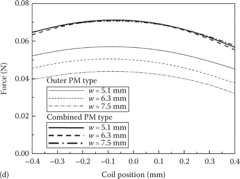
The examples in Figure 17.5a and b show flux distribution [4]; the flux density and thrust versus coil position (height h₂ in mm) are illustrated in Figure 17.5c. They are typical of the efficacy of 2D FEM for the scope.

For h₁ = 1.1 mm, the PM flux in the coil is most symmetric, as it should. The average PM flux density over the coil height pulsates inevitably with the coil position, when the latter vibrates. The force variation with coil position is a clear indication of this phenomenon.

The average PM flux density (ac component) contributes to the pure sinusoidal SPL, with sinusoidal current. The harmonics lead to harmonics distortion.

PM height h₂, coil position h₁, and central to the outer membrane diameter ratio, coil height and total airgap may be considered in an optimization design, where the sound pressure should be maximized and THD and volume should be constraint.

To obtain sound power W_rad(f), however, the speed of coil $\dot{x} (f)$ $\dot{x} (f)$ should be calculated. Consequently, a dynamic model is required. The latter includes the voltage and motion equations:

\frac{d i}{d t} = \frac{V - i R - K_{e} (x) \dot{x}}{L} (17.32)

$\frac{d i}{d t} = \frac{V - i R - K_{e} (x) \dot{x}}{L} (17.32)$

Images

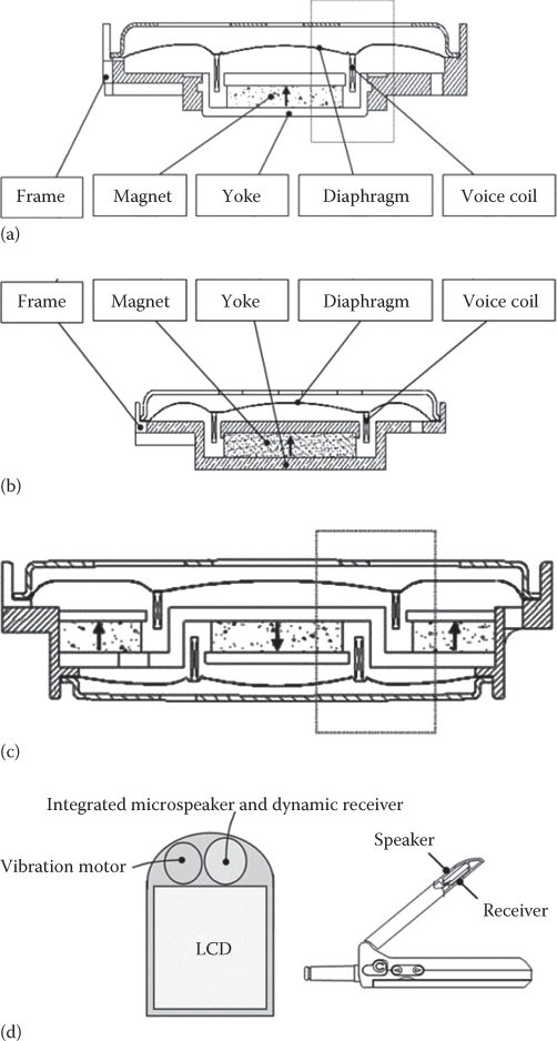
FIGURE 17.4 (a) Microspeaker alone, (b) receiver alone, (c) integrated microspeaker and dynamic receiver, and (d) layout of integrated device. (After Hwang, S.M. et al., IEEE Trans., MAG-39(5), 3259, 2003.)

\dot{x} = \frac{K_{e} (x) i - C \dot{x} - K x}{M} (17.33)

$\dot{x} = \frac{K_{e} (x) i - C \dot{x} - K x}{M} (17.33)$

C is the dynamic factor

K is the spring factor

M is the mover mass

R, L are the coil resistance and inductance

V is the supply (or input) voltage

Images

FIGURE 17.5 (a) Integrated device components, (b) flux distribution, and (c) PM flux density in the coil airgap. (d) Typical force/coil position dependence. (After Hwang, S.M. et al., IEEE Trans., MAG-39(5), 3259, 2003.)

Images

The emf (and thrust) coefficient, K_e(x), may be obtained from 2D FEM by curve fitting. Either with sinusoidal voltage (for the speaker) or sinusoidal motion (for the dynamic receiver), model equations (17.32) through (17.33) may be solved numerically.

Subsequently, the SPL (dB) and THD (%) may be calculated. They also may be measured (Figure 17.6).

Typical results [4] are shown in Figure 17.7.

Images

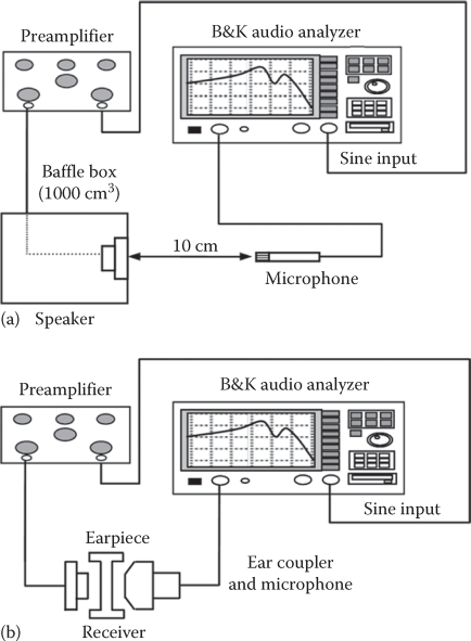
FIGURE 17.6 Test rig for: (a) speaker SPL and (b) receiver SPL. (After Hwang, S.M. et al., IEEE Trans, MAG-39(5), 3259, 2003.)

Images

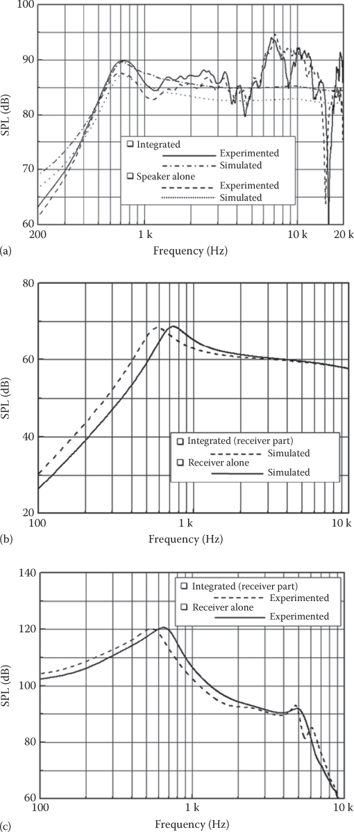
FIGURE 17.7 Sound pressure for speakers (a), receiver in open air (b), in an auspice (c). (After Hwang, S.M. et al., IEEE Trans., MAG-39(5), 3259, 2003.)

A satisfactory agreement between digital simulations and experiments is accompanied by the visible large frequency band (0.5–4 kHz at least), due to the proper electromagnetic design of the coil-mover LOM.

17.3 PM-MOVER LOM(G)

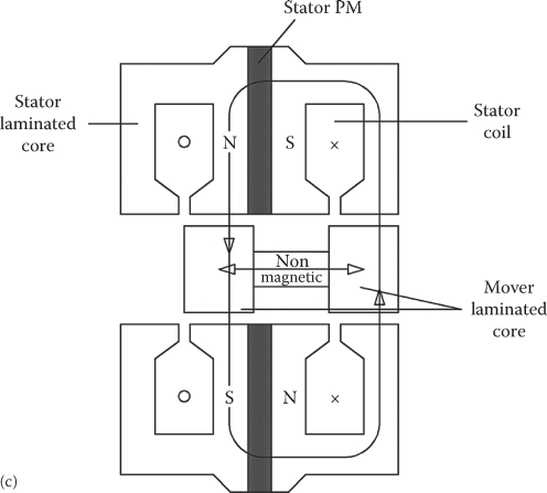
There are two fundamental topology options: tubular or flat. From the tubular option, we present here only ones with surface single (homopolar)- or multiple-PM pole mover, with single- and multiple-coil stator, respectively (Figures 17.8 and 17.9) [6–10].

The configurations with 1(2) stator coils are preferable for pancake shape (large diameter and short length), while the multiple-PM, multiple-coil topologies are typical for longer with smaller-diameter volumes.

In single- and multiple-coil stators (one coil per one PM pole in the rotor), the PM flux linkage switches polarity.

The homopolar PM mover (Figure 17.8a) is used commercially, and thus it will be investigated here in some detail first. The two Halbach PM pole topology [9] (Figure 17.8c) that claims a reduction of mover weight is supposed to contain also a thinner magnetic core; however, the attached core weight increases notably the size and cost of the mechanical springs and limits the eigenfrequency to 50–60 Hz.

Images

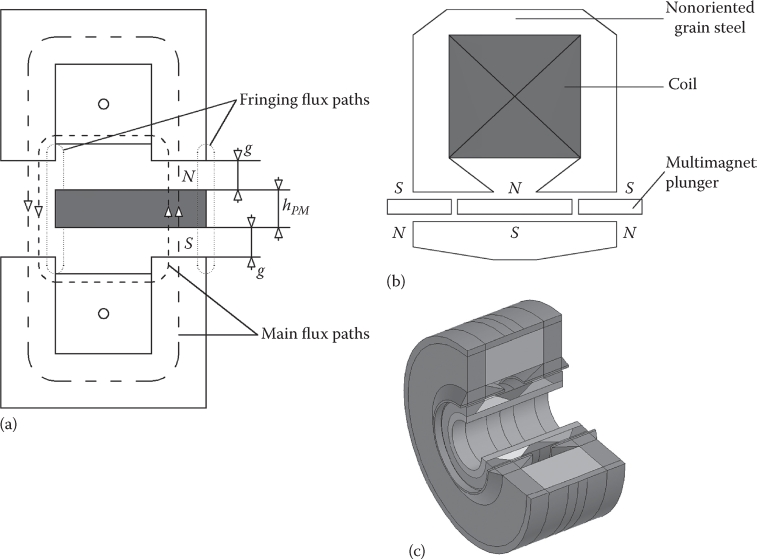
FIGURE 17.8 Tubular PM-mover LOM(G)s, (a) with single (homopolar) PM pole mover and stator coil. (After Wang, J. et al., Comparative study of winding configurations of short-stroke, single phase tubular permanent magnet motor for refrigeration applications, Conference Record of the IEEE Industry Applications Society Annual Meeting (IEEE-IAS’2007), New Orleans, LA, 2007; Redlich, R.W. and Berchowitz, D.H., Proc. Inst. Mech. Eng., 199(3), 203, 1985.) (b) and (c) with dual-pole PM mover and single- and dual-stator coil. (After Ibrahim, T. et al., Analysis of a short-stroke, single-phase tubular PM actuator for reciprocating compressors, 6th International Symposium on Linear Drives for Industrial Applications (LDIA2007), Lillie, France, 2007.)

Images

FIGURE 17.9 LOM(G): Tubular multiple PM-pole mover and multiple-coil stator topology: (a) cross section, (b) two PM poles, (c) radial PMs, (d) slits, and (e) flexures.

Although less rugged (mechanically), the “pure” PM mover with nonmagnetic lightweight (siluminum or resin) framing is considered here further as it allows a reasonable mechanical spring for high enough eigenfrequencies (up to 300 Hz for 50 W devices).

The cogging force of yet another variant of the single-stator-coil three-pole PM mover is shown in Figure 17.10; it is apparently capable of producing a linear cogging force, sufficient to replace the mechanical spring if 25% of the ideal maximum stroke length is “sacrificed” [11].

The tubular configurations are credited with the blessing of the circularity, and using “flexures” (Figure 17.9) as mechanical springs, both the resonance conditions and the linear bearing functions are performed.

On the other hand, a flat but double-sided topology, eventually with PM flux concentration, with square-like stator coil shape may allow a more rugged PM mover and a higher force (power) density. A so-called flux reversal of such topology is shown in Figure 17.11.

The double-sided structure provides for ideally zero normal force on the mover (when placed central in the airgap) and all PM utilization all the time.

The rather large PM flux leakage and fringing are inevitable. This situation is also typical for tubular single-coil single-PM-mover configurations (Figure 17.8a).

The stroke length in all PM-mover LOMs is rather small (less than 20 mm in general); the theoretical maximum stroke length corresponds to the motion length that leads to maximum positive maximum negative PM flux in the stator coil(s)—or the pole pitch τ = x_max = l_stroke.

In what follows, we will treat in some detail three PM-mover LOM topologies: the tubular homopolar PM mover, the tubular multiple-PM pole mover with multiple stator coils, and the flat double-sided flux-reversal PM-mover LOM(G).

17.3.1 Tubular Homopolar LOM(G)

A low-power high-frequency (f_e = f_m = 300 Hz) tubular homopolar PM-mover LOM is illustrated in Figure 17.12, where the stator is the interior part (to reduce copper losses) and the cores are made of SMC (somaloy 700 or better).

To thoroughly investigate such a configuration, considering radial and axial eccentricities, a 3D electromagnetic field model is needed. This was done [12] with remarkable success.

Images

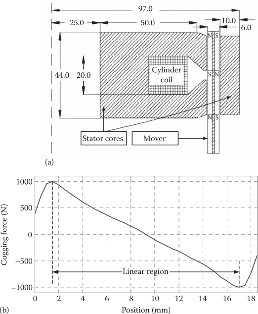
FIGURE 17.10 (a) Potentially spring-less tubular PM-mover LOM(G) and (b) with its cogging force (“magnetic” spring). (After Boldea, I. et al., Springless resonant linear oscillatory PM motors? International Symposium on Linear Drives for Industrial Applications (LDIA2011), Eindhoven, the Netherlands, 2011.)

Images

FIGURE 17.11 Flat flux-reversal PM-mover LOM(G) with PM flux concentration (double sided). (After Pompermaier, C. et al., Analytical and 3D FEM modeling of a tubular linear motor taking into account radial forces due to eccentricity, IEEE International Electric Machines and Drives Conference (IEMDC’09), Miami, FL, 2009.)

However, to investigate the machine dynamics, with reasonable computation effort, a practical magnetic circuit model may be used (Figure 17.13a), with flux lines illustrated in Figure 17.13b. To account for PM flux fringing and leakage—which is paramount—the magnetic circuit should be modified with mover position a few times.

As an example, the magnetic reluctances of flux lines 1 and 6 (in Figure 17.13) are

R_{l i n e l} \approx \frac{g + t}{2 μ_{0} t_{m} (2 r_{a} + g)} (17.34)

$R_{l i n e l} \approx \frac{g + t}{2 μ_{0} t_{m} (2 r_{a} + g)} (17.34)$

Images

FIGURE 17.12 Tubular homopolar PM-mover LOM with interior single-coil stator. (After Pompermaier, C. et al., IEEE Trans, IE-59(3), 1389, 2012.)

Images

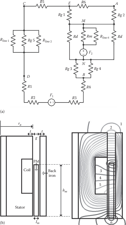
FIGURE 17.13 Magnetic circuit, (a) fringing (1,2) and (b) leakage (3,4,5) PM flux line tubs. (After Pompermaier, C. et al., IEEE Trans, IE-59(3), 1389, 2012.)

R_{l i n e 6} \approx \frac{1}{2 π μ_{0} h_{m}} \log (\frac{r_{a} + l_{m}}{r_{a}}) (17.35)

$R_{l i n e 6} \approx \frac{1}{2 π μ_{0} h_{m}} \log (\frac{r_{a} + l_{m}}{r_{a}}) (17.35)$

The airgap flux Φ (traversing R_g₅ in Figure 17.13a) is approximately

Φ = \frac{F_{m m 1} - (R_{d} | | 2 R_{b}) F_{m m 2}}{R_{a} + R_{g 1} | | (R_{6} + R_{g 2}) + R_{m} | | (R_{g} / 2) + R_{g 3} | | R_{g 4}}; F_{w m 1} = N i; F_{m m 2} = l_{m} \frac{B_{r}}{μ_{0}} (17.36)

$Φ = \frac{F_{m m 1} - (R_{d} | | 2 R_{b}) F_{m m 2}}{R_{a} + R_{g 1} | | (R_{6} + R_{g 2}) + R_{m} | | (R_{g} / 2) + R_{g 3} | | R_{g 4}}; F_{w m 1} = N i; F_{m m 2} = l_{m} \frac{B_{r}}{μ_{0}} (17.36)$

R_{a} = R_{1} + R_{2} + R_{3} + R_{4} + R_{g 5} + R_{g 6}; R_{b} = \frac{R_{a}}{2} + R_{m} (17.37)

$R_{a} = R_{1} + R_{2} + R_{3} + R_{4} + R_{g 5} + R_{g 6}; R_{b} = \frac{R_{a}}{2} + R_{m} (17.37)$

The nonlinear B(H) curve of SMs is considered and the flux Φ is calculated iteratively. R_m is the PM magnetic reluctance and R_d is the PM leakage reluctance.

The emf is

e m f = - N \frac{d Φ}{d t} = - N \frac{d Φ}{d t} \frac{d x}{d t} = - N K_{e} (x) \frac{d x}{d t} (17.38)

$e m f = - N \frac{d Φ}{d t} = - N \frac{d Φ}{d t} \frac{d x}{d t} = - N K_{e} (x) \frac{d x}{d t} (17.38)$

Typically, emf results obtained via the analytical 2D FEM and by experiments are compared in Figure 17.14.

Therefore, the magnetic circuit method is reliable to calculate emf, and, consequently, the interaction thrust F_x also:

F_{x} = N \frac{d Φ}{d x} i = N K_{e} (x) i (17.39)

$F_{x} = N \frac{d Φ}{d x} i = N K_{e} (x) i (17.39)$

The cogging force has to be calculated by FEM, and its variation with displacement (in Figure 17.15a) suggests that it is trying to expel the mover outside the airgap (it is negative for negative displacement):

Thus, it opposes the spring action.

Images

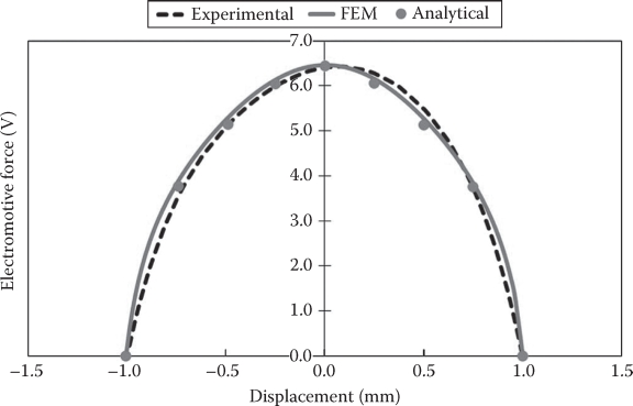
FIGURE 17.14 Emf: computed versus experimental results. (After Pompermaier, C. et al., IEEE Trans., IE-59(3), 1389, 2012.)

Images

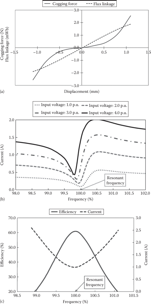
FIGURE 17.15 (a) Cogging force, (b) current versus resonance frequency $(f_{m} = \sqrt{K / M})$ $(f_{m} = \sqrt{K / M})$ , and (c) expecting efficiency and current. (After Pompermaier, C. et al., IEEE Trans., IE-59(3), 1389, 2012.)

This shows in the reduction of resonance frequency (Figure 17.15b), when the input voltage increases (which means also larger stroke length [larger load]) and when the cogging force is larger. The reduction of stroke with load reduction takes place at resonance frequency and thus at good efficiency.

At resonance, the current is minimum and efficiency is maximum (Figure 17.15c). The rather modest 60% efficiency may be justified by the rather low power (20–30 W), in a very small volume device. As already visible, the resonance frequency varies a little due to cogging force, but it also does with spring aging, temperature, etc. The presence of a single-phase inverter and a slow minimum-current close loop to adjust the reference inverter frequency solves this problem.

Operation at grid frequency—which varies by up to 0.1–0.2 Hz (at least) during the day—would lead to notable variations in the average efficiency of the LOM(G)s.

17.3.2 25 W, 270 Hz, Tubular Multi-PM-Mover Multi-Coil LOM: Analysis by Example

In this paragraph a rather detailed analytical FEM and dynamics modeling and analysis are unfolded to provide a more complex view of the technology under scrutiny.

The configuration is that of Figure 17.9, with the following specifications:

P_n = 25 W (motor)
Stroke length l_stroke=6 mm (±3 mm)
Frequency f₁ ≤ 270 Hz
Outer diameter D_OS < 16 mm
DC input voltage V_dc = 12 V_dc (inverter supply)

The following analysis issues are followed here:

General design, optimization design, FEM analysis, simplified linear circuit model for steady state and transients, and a nonlinear circuit model with MATLAB^® code for dynamics and control

17.3.2.1 General Design Aspects

With 1 W (4%) of mechanical losses, the electromagnetic power P_en is

P_{e n} = P_{n} + P_{m e c h l o s s} = 25 + 1 = 26 W (17.40)

$P_{e n} = P_{n} + P_{m e c h l o s s} = 25 + 1 = 26 W (17.40)$

The average linear speed and the stroke length l_stroke are

u_{a v} = 2 \cdot l_{s t r o k e} \cdot f_{1} = 2 \cdot 6 \cdot 10^{- 3} \cdot 270 = 3.24 m/s (17.41)

$u_{a v} = 2 \cdot l_{s t r o k e} \cdot f_{1} = 2 \cdot 6 \cdot 10^{- 3} \cdot 270 = 3.24 m/s (17.41)$

l_{s t r o k e} = 2 \cdot 3 = 6 mm = 6 \cdot 10^{- 3} m (17.42)

$l_{s t r o k e} = 2 \cdot 3 = 6 mm = 6 \cdot 10^{- 3} m (17.42)$

The average thrust is

F_{x a v} = \frac{P_{e n}}{u_{a v}} = \frac{26}{3.24} = 8.2 N (17.43)

$F_{x a v} = \frac{P_{e n}}{u_{a v}} = \frac{26}{3.24} = 8.2 N (17.43)$

Choosing an average thrust surface density f_s = 0.64 N/cm² and a stator bore diameter D_is ≈ 0.5 D_os = 8 mm, the required stator length L_s is

L_{s} = \frac{F_{a v}}{π \cdot D_{i s} \cdot f_{s}} \approx 50 mm (17.44)

$L_{s} = \frac{F_{a v}}{π \cdot D_{i s} \cdot f_{s}} \approx 50 mm (17.44)$

The airgap PM flux density B_agv has two components:

B_{g a v} = B_{P M r} + B_{P M a} (17.45)

$B_{g a v} = B_{P M r} + B_{P M a} (17.45)$

which correspond to radially and, respectively, axially magnetized PMs.

Approximately

B_{P M r} = B_{r} \frac{h_{P M}}{(h_{P M} + g μ_{r e c}) (1 + k_{s}) (1 + k_{f r})} (17.46)

$B_{P M r} = B_{r} \frac{h_{P M}}{(h_{P M} + g μ_{r e c}) (1 + k_{s}) (1 + k_{f r})} (17.46)$

B_{P M a} = B_{r} \frac{1}{(\frac{2 g}{l_{P M}} + \frac{τ}{2 h_{P M}}) (1 + k_{f a})} (17.47)

$B_{P M a} = B_{r} \frac{1}{(\frac{2 g}{l_{P M}} + \frac{τ}{2 h_{P M}}) (1 + k_{f a})} (17.47)$

With B_r = 1.2 T, µ_rec = 1.07 p.u., g = 0.3 mm, h_pm = 1.2 mm, k_s = 0.1 (saturation factor), kfr=0.2 (fringing factor for radial PMs), and k_fa = 2 (fringing factor for axially magnetized PMs), we get B_PMa = 0.124 T, B_PMr=0.85 T. The ratio B_PMa/B_PMr=0.124/0.85 ≈ 0.15 = 15% represents the additional thrust proportion brought by the axially magnetized PMs.

Skipping design details, for V_n = 12 Vdc, we end up with the following PM-LOM parameters: Emf (peak value) ≈ 0.49 ∙ w_c. (w_c, turns per coil; N = 6 coils, only 5 coils are fully active). The two end coils experience only homopolar PM flux variations, so they “account” to one fully active coil. In such conditions, the number of turns per coil w_c = 20 turns and rated current is 5.2A.

The inductance is $L_{s} \approx 0.28 \cdot 10^{- 6} w_{c}^{2} = 0.112 \cdot 10^{- 3} H$ $L_{s} \approx 0.28 \cdot 10^{- 6} w_{c}^{2} = 0.112 \cdot 10^{- 3} H$ , and the resistance $R_{s} = 9.52 \cdot 10^{- 4} w_{c}^{2} = 0.3772 Ω$ $R_{s} = 9.52 \cdot 10^{- 4} w_{c}^{2} = 0.3772 Ω$ .

The electric time constant T_e = L_s/R_s = 0.3 ms, which implies 20 kHz or more PWM switching frequency. The copper losses p_con = 6.868 W (J_co = 20 A/mm²) and the iron losses p_iron = 2.47 W (Somaloy 54 W/kg at 1 T and 270 Hz) lead to efficiency η_n = 0.7075 (an improved 74% efficiency will be obtained by optimization design and then validated by FEM when the mover and the stator core losses will be checked). A rather complete circuit model including the mover losses (attributed in the stator) is shown in Figure 17.16; R_PM is the PM eddy current resistance and R_imov is the rotor solid back iron resistance. After key FEM validations and corrections of the analytical model used earlier, in the general design, by fudge factors, optimization design proceeds.

Images

FIGURE 17.16 Complete circuit model of PM LOM.

17.3.2.2 Optimization Methodology by Example

Optimization design methodology and MATLAB code include a few distinct stages as seen from the input file summarized in Table 17.1.

There are imposed “primary dimensions,” “technical requests,” “technical limitations,” initial values of “optimization variables and limits for them,” “objective function coefficients,” “step size,” and other specifications such as stator winding and rotor temperature limitations. An improved “Hooke-Jeeves” optimization method is used and the objective function is

F_{o b} = c_{1} \frac{p_{c o} + p_{i r o n}}{p_{l o s s 0}} + c_{2} \frac{m_{m o v e r}}{m_{m o v e r 0}} (17.48)

$F_{o b} = c_{1} \frac{p_{c o} + p_{i r o n}}{p_{l o s s 0}} + c_{2} \frac{m_{m o v e r}}{m_{m o v e r 0}} (17.48)$

where

p_loss0 are the electric losses

m_mover0 is the weight of the mover, both from the initial design

c₁, c₂ are proportionality coefficients chosen by trial and error (Table 17.1)

The objective function is a compromise between electric losses and mover’s weight as the latter influences the mechanical spring size (weight) and cost.

TABLE 17.1
Given Parameters in the Input File of the Optimization Design Code

Images

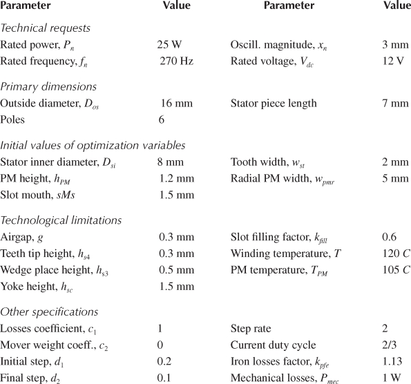
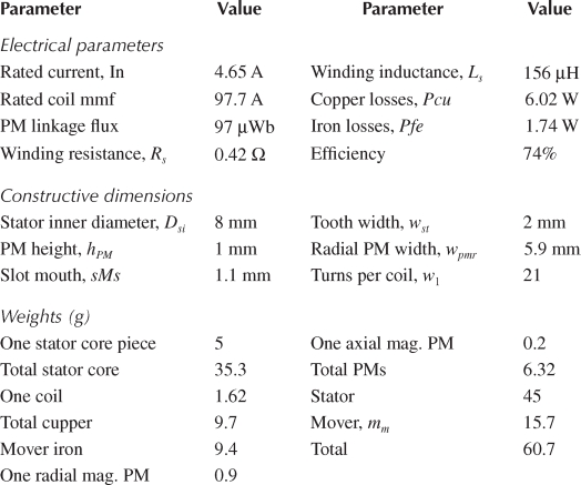
TABLE 17.2
Computed Parameters from Output File Optimization Design Code

Images

The Hooke–Jeeves optimization algorithm is a pattern search algorithm using two kinds of moves: exploratory moves and pattern moves. Five optimized variables (Table 17.1.) are grouped in a vector, and each element is modified with a given step in the exploratory moves. The objective function gradient is computed and after that, the algorithm starts pattern moves until the objective function reaches a minimum. From that point on, another search move is started. If there is not a smaller value for the objective function, then the step is decreased in ratio of step rate. The algorithm is stopped after the final step d₂ (Table 17.2) is reached. At each step, the optimization variables are limited within their range.

As the motor is supposed to be cooled together with the linear piston compressor, the 120° winding temperature is used only to calculate the copper losses.

A sample output file is summarized in Table 17.2, where we can see a 4% improvement in the efficiency from 70% in the initial design, to 74%, with a total motor weight of 60 g without mechanical springs.

The number of iterations needed for a given progress ratio in the optimization was around 10 and computation CPU time was 9.35 s (on a dual core 2.4 GHz processor, Windows XP, MATLAB 6.5). The same optimization design was run for f₁ = 500 Hz; a very tempting efficiency η_n=0.82% for 58 g of active materials and the same 6(±3) mm stroke length was obtained. If a mechanical spring for this eigenfrequency (500 Hz) can be built (mover weight ≈11 g), then the 500 Hz solution might be preferable.

17.3.2.3 FEM Analysis

A 2D FEM analysis of the tubular configuration has been performed to validate PM flux density distribution, emf, thrust, and rotor losses. The results on PM airgap flux density distribution with position for three mover positions (x=0 means mover in the middle position), Figure 17.17, shows rather high levels, as required. Saturation “hot-spot” places have been kept also within limits to limit core losses (stator: Somaloy core; the mover back iron: mild solid steel). The 0.83 T average of PM airgap flux density value from the initial design is also confirmed.

Images

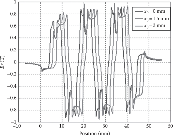
FIGURE 17.17 Airgap radial PM flux density distribution in the middle of the airgap.

The total force at constant mmf versus position, shown in Figure 17.18, proves that the PM LOM is capable of producing the required average thrust of 8 N. It also shows that there is a cogging force (zero current force) that manifests itself as a virtual nonlinear spring.

The thrust decreases toward excursion’s end, but in reality, as the mmf is in phase with the speed (sinusoidal (harmonic) motion—imposed mainly by the mechanical springs) and with the current, the thrust has to go anyway down to zero at excursion’s end. The average electromagnetic power (F_x(x) ∙ u(x)) for sinusoidal motion, constant current, is shown in Figure 17.19 for both 270 and 500 Hz PM-LOM operation.

Typical FEM emf waveform for one turn/coil is shown in Figure 17.20, for harmonic motion at 270 Hz, with its frequency spectrum.

The FEM calculated inductance is shown in Figure 17.21. It depends on mover position and on mmf (load) but, in fact, on local magnetic saturation. Its average value (at rated 102 A turns/coil) is about equal to the 0.11 mH analytically calculated value (w_c = 20 turns/coil) in the initial design.

To check the level of mover eddy current losses, the latter have been investigated by FEM at standstill for the rated (270 Hz) frequency of the sinusoidal rated stator current (102 A turns/coil). Their distribution is shown in Figure 17.22a (p_Fe = 10 ρ_Co, ρ_PM = 1.2 ∙ 10⁻⁶ Ωm, µ_riron = 730 p.u.), and the eddy current density variation along mover outer surface is evident in Figure 17.22b. The mover eddy current losses are (at 270 Hz) 16.4 mW in PM and 33.5 mW in the mover solid back iron. These values are rather small with respect to the total core losses of 2.4 W considered in the analytical design model, but still worthy of consideration as they are about 2% of all core losses.

Note: At 25 W, (500 Hz), the mover eddy current losses are slightly smaller than for 270 Hz because the stator current (the main source of these losses) is notably smaller (because efficiency is better).

17.3.2.4 Simplified Linear Circuit Model for Steady State and Transients

For sinusoidal current and sinusoidal motion (and emf), a simplified circuit model can be developed considering the single-phase linear PMSM with a cage-less PM mover.

Images

FIGURE 17.18 (a) Total thrust and (b) current-interaction force for constant coil mmf.

Thus, for sinusoidal steady state, at resonance $(ω_{1} = ω_{r e s}; ω_{r e s} = \sqrt{k_{s p r i n g} / m_{m}})$ $(ω_{1} = ω_{r e s}; ω_{r e s} = \sqrt{k_{s p r i n g} / m_{m}})$ , the PM-LOM equations are

\begin{array}{l} {\underline{V}}_{1} = R_{s} {\underline{I}}_{1} + J ω_{1} L_{s} {\underline{I}}_{1} + {\underline{E}}_{1} \\ {\underline{E}}_{1} = k_{e} {\underline{U}}_{1} \end{array} (17.49)

$\begin{array}{l} {\underline{V}}_{1} = R_{s} {\underline{I}}_{1} + J ω_{1} L_{s} {\underline{I}}_{1} + {\underline{E}}_{1} \\ {\underline{E}}_{1} = k_{e} {\underline{U}}_{1} \end{array} (17.49)$

F_{x} = k_{e} I_{1} (17.50)

$F_{x} = k_{e} I_{1} (17.50)$

For transients we consider that the average load is proportional to speed:

F_{l o a d} (t) \approx C_{l o a d} U (t) (17.51)

$F_{l o a d} (t) \approx C_{l o a d} U (t) (17.51)$

Images

FIGURE 17.19 Average electromagnetic power versus position at constant mmf per coil (in A) (a) f₁ = 270 Hz, (b) f₁ = 500 Hz.

We may rewrite now the voltage and motion equations for transients:

V_{1} (t) = R_{s} i (t) + L_{s} \frac{d i}{d t} + k_{E} u (t) (17.52)

$V_{1} (t) = R_{s} i (t) + L_{s} \frac{d i}{d t} + k_{E} u (t) (17.52)$

m \frac{d u (t)}{d t} = k_{E} i (t) - k_{s p r i n g} x (t) - C_{l o a d} u (t) (17.53)

$m \frac{d u (t)}{d t} = k_{E} i (t) - k_{s p r i n g} x (t) - C_{l o a d} u (t) (17.53)$

Images

FIGURE 17.20 Emf for one turn/coil versus (a) time for harmonic motion and (b) its harmonic spectrum.

The cogging force is neglected in the transient model here. With sinusoidal voltage and steady-state motion

\underline{V_{1}} = V_{1} {\sqrt{2 e}}^{j ω_{1} t}; \underline{U_{1}} = J ω_{1} {\underline{X}}_{1} (17.54)

$\underline{V_{1}} = V_{1} {\sqrt{2 e}}^{j ω_{1} t}; \underline{U_{1}} = J ω_{1} {\underline{X}}_{1} (17.54)$

\underline{I_{1}} = \frac{{\underline{X}}_{1} (k - ω_{1}^{2} m + j ω_{1} C_{l o a d})}{k_{E}} = {\underline{U}}_{1} {(\frac{C_{l o a d}}{k_{E}})}_{ω_{1} = ω_{r e s}} (17.55)

$\underline{I_{1}} = \frac{{\underline{X}}_{1} (k - ω_{1}^{2} m + j ω_{1} C_{l o a d})}{k_{E}} = {\underline{U}}_{1} {(\frac{C_{l o a d}}{k_{E}})}_{ω_{1} = ω_{r e s}} (17.55)$

Images

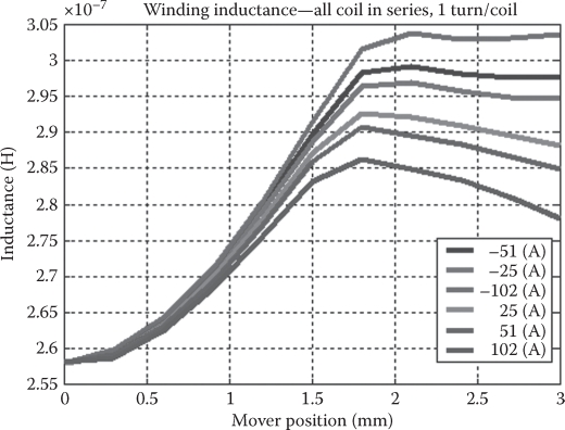
FIGURE 17.21 Inductance versus mover position for various coil mmf’s.

For transients in Laplace form, the earlier equalities become

\begin{array}{l} {\tilde{V}}_{1} = (R_{s} + s L_{s}) \tilde{i} + k_{E} s \tilde{x} \\ m s^{2} \tilde{x} = k_{E} \tilde{i} - k_{s p r i n g} \tilde{x} - C_{l o a d} s \tilde{x} \end{array} (17.56)

$\begin{array}{l} {\tilde{V}}_{1} = (R_{s} + s L_{s}) \tilde{i} + k_{E} s \tilde{x} \\ m s^{2} \tilde{x} = k_{E} \tilde{i} - k_{s p r i n g} \tilde{x} - C_{l o a d} s \tilde{x} \end{array} (17.56)$

\tilde{x} = \frac{k_{E} \tilde{V}}{(R_{s} + s L_{s}) (s^{2} m + s C_{l o a d} + k_{E}) s k_{E}^{2}} (17.57)

$\tilde{x} = \frac{k_{E} \tilde{V}}{(R_{s} + s L_{s}) (s^{2} m + s C_{l o a d} + k_{E}) s k_{E}^{2}} (17.57)$

All the roots of the denominator in (17.57) have negative real parts, so the response to any voltage input is always stable. Consequently, starting the PM LOM by applying directly the voltage at resonance frequency is the way to follow. Also, for reduced load, only the voltage amplitude has to be reduced: it just reduces the excursion length and thus also the current.

This would be similar to the ideal case when, in rotary machines, we could hypothetically modify continuously the pole pitch (l_stroke = pole pitch, here).

This seems a simple and efficient way to handle variable capacity refrigeration (or other loads).

This simplified dynamic model has served only as basis for insights and for steady-state performance calculation under load.

To illustrate its usefulness, we show in Figure 17.23 the displacement and sinusoidal current magnitudes (Figure 17.23a and b) and the output average power versus frequency (Figure 17.23c).

The beneficial effect of resonance conditions is evident. The presence of the inverter can help to follow on line the eventual slow variations of spring eigenfrequency due to temperature and mechanical aging, by just hunting slowly for minimum current at given load.

17.3.2.5 Nonlinear Circuit Model and MATLAB® Code with Digital Simulation Results

The analytical model for steady state and transients in the previous paragraph did not account precisely for actual thrust/current/position or cogging force/position curves. Therefore, especially when the stroke is above 50% of maximum value, the simplified circuit model loses much in precision (F_x=k_ei; k_e is in reality a function of mover position). If we import k_e(x,t), the emf shape, introduce cogging force (all from FEM), and add also Coulomb’s friction influence, we obtain a nonlinear circuit model (even with neglected magnetic saturation), which, in MATLAB–Simulink®, looks as in Figure 17.24.

Images

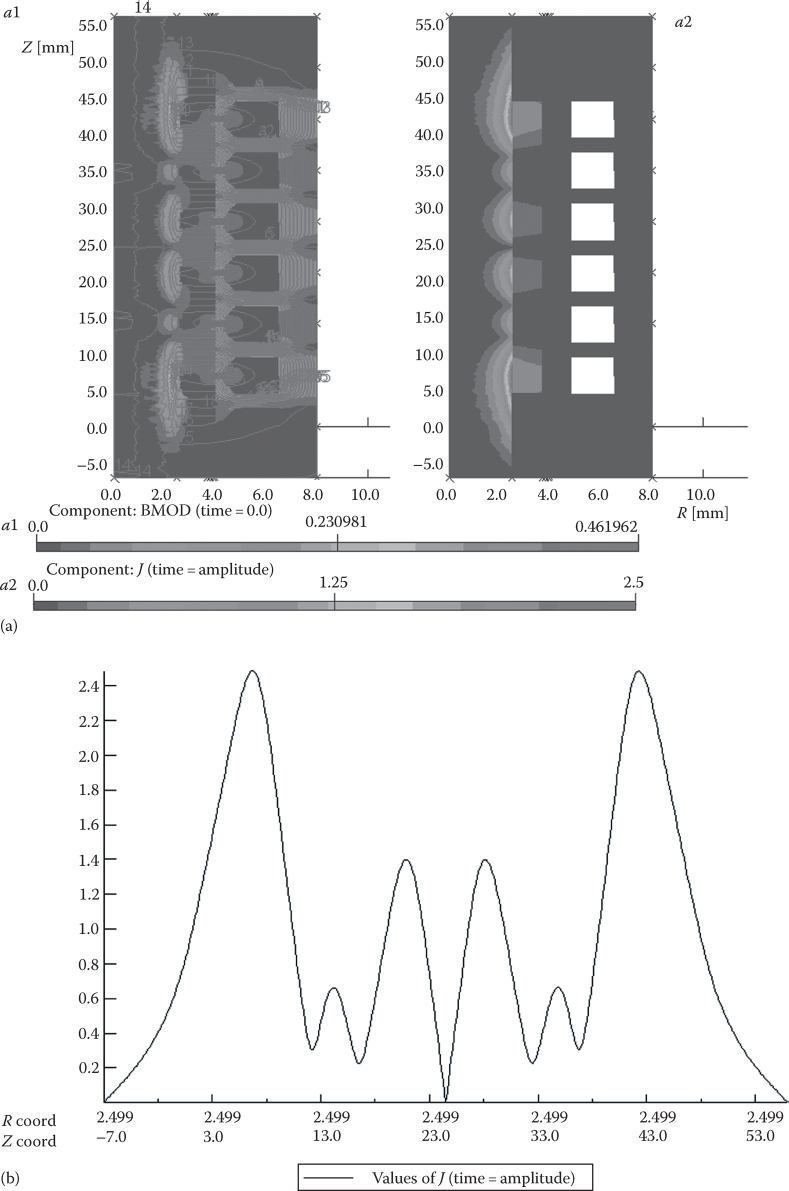
FIGURE 17.22 Mover eddy currents distribution at standstill with ac rated current (a) and current density variation along mover outer surface (b).

A very rigid fictitious spring (material) is added in the model to “reflect” the mover accidental “exit” beyond stroke ends.

With this nonlinear model, voltage open-loop and current close-loop controls are explored. Only a few sample results are given here (due to lack of space).

Images

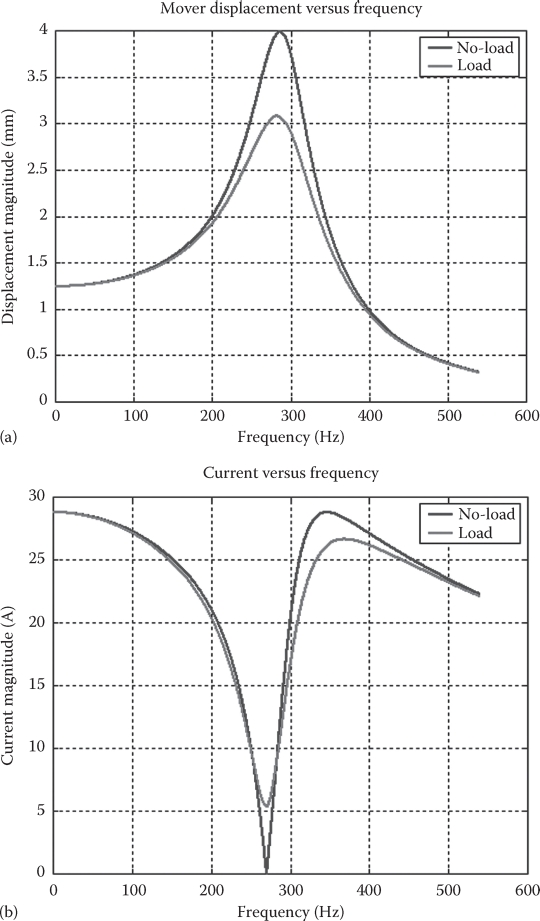
FIGURE 17.23 Sinusoidal voltage and motion steady-state characteristics versus frequency (a) displacement, (b) current, (c) output average power.

Images

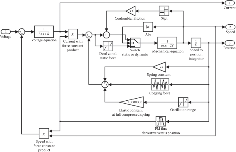
FIGURE 17.24 Proposed nonlinear model of PM-LOM.

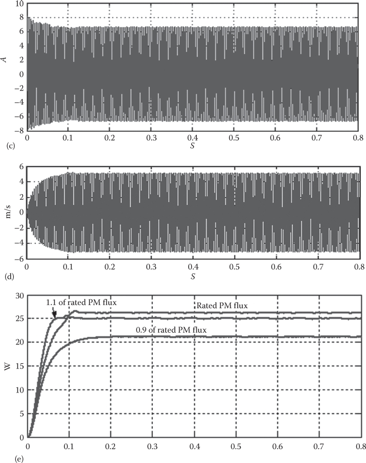
Direct starting and operation under load at constant (resonance) frequency with open-loop gradual voltage application is shown in Figure 17.25a through d (voltage amplitude, current waveform, instantaneous speed, and average power).

The MATLAB-Simulink solver automatically chooses the sampling time to keep the relative errors smaller than 10⁻⁴. The PWM signal is generated by a modified sigma-delta modulator that contains a zero-order hold with 2 µs sampling time in its local close loop.

Images

FIGURE 17.25 Gradual open-loop voltage application for start at 270 Hz: (a) voltage amplitude, (b) current, (c) speed, and (d) average power versus time.

The control objective of the linear motor is to obtain maximum efficiency for compressor drives or to precision tracking if it is used as an actuator.

Sinusoidal close current loop control at mechanical resonance frequency, for maximum efficiency, was also investigated, with satisfactory results for voltage, current, speed, and average power (Figure 17.26).

A zoom on steady state for voltage, current, and speed would show very clearly the resonance conditions (the current is almost in phase with speed). The current control loop is of on-off type with the application of ±V_dc (dc voltage). The sampling time for zero order hold is set at 20 µs in this case to limit the maximum switching frequency at 25 kHz and keep the current ripple within an acceptable range (Figure 17.26b). The current control is robust to electrical parameters uncertainly. The output power variation is practically not sensitive to a large winding resistance and inductance variation. It has an acceptable sensitivity with respect to permanent magnet flux as shown in Figure 17.26e. There is a notable sensitivity to mechanical parameters (mover total mass and mechanical spring constant). For example, increasing the spring rigidity by 10% the output power will decrease at 13.5 W, while decreasing the spring stiffness at 90% will decrease the output power to only 7.7 W. To track the small changes in resonant frequency, the frequency synthesized by the inverter is changed in order to drive the phase angle between current and emf to zero (a simple voltage model would provide good emf estimation because the frequency is rather large). This aspect is beyond our scope here.

Images

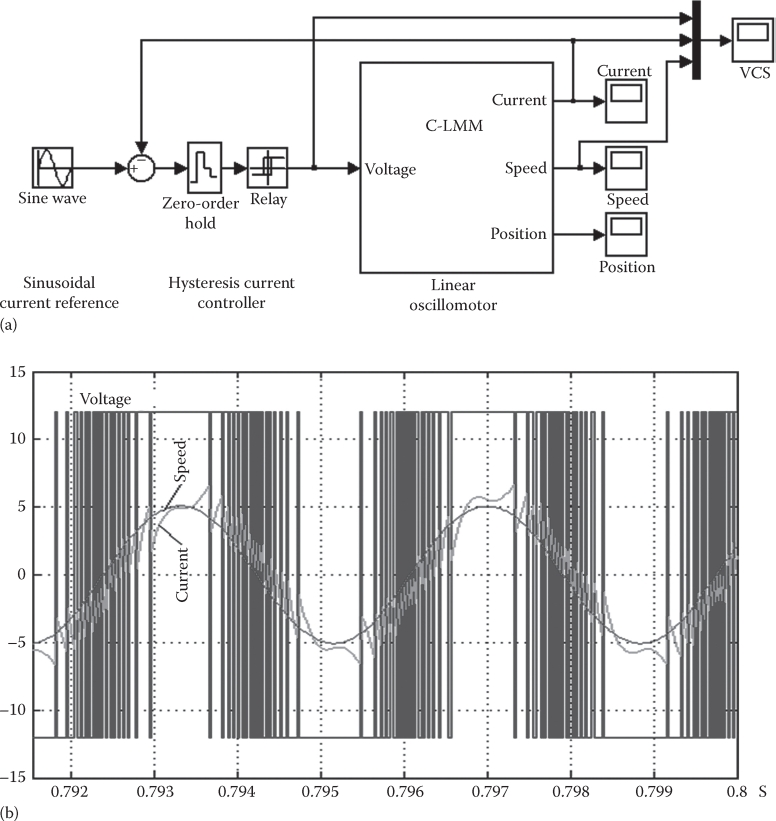
FIGURE 17.26 Close-loop sinusoidal current control: (a) genetic control, (b) current and speed versus time (zoom), (c), (d) current and speed, and (e) output average power in W, during acceleration speed-proportional load.

Images

Comparing Figures 17.25 and 17.26, we may infer that much faster starting is achieved with close-loop current control (from 0.25 to 0.1 s), though in both cases (open-loop and close-loop current control) successful synchronization under full load is obtained. To modify the refrigeration capacity, the reference voltage (respectively, current) is changed. Close-loop current control is to be preferred as it is less dependent on machine parameters.

17.3.3 Double-Sided Flat PM-Mover LOM

In this paragraph, two built prototypes are investigated: one with surface and one with interior PM mover [13,14]. The scope is to model and characterize them thoroughly both for steady state and for dynamic operation.

The prototypes’ configurations are shown in Figure 17.27. The mover is sliding on linear bearings and the kinetic energy is recovered by two mechanical springs.

The main dimensions of the prototypes are

Stroke length: 10 mm
Teeth width: 5 mm
Airgap: 1 mm
Permanent magnet thickness: 2 mm
Permanent magnet material is NdFeB with B_r = 1.13–1.18 T, H_c = 844–900 kA/m
Number of turns/coil: 285
Wire diameter: 0.45 mm
Mover mass: 2 kg

17.3.3.1 State-Space Model of the Linear Machine

The model of the linear machine is based on voltage and mechanical differential equations:

V = R I + \frac{d Ψ}{d t} (17.58)

$V = R I + \frac{d Ψ}{d t} (17.58)$

Images

FIGURE 17.27 Prototypes configurations: (a) surface PM mover and (b) internal PM mover.

m \frac{d u}{d t} = F_{e m} - F_{c g} - F_{l o a d} - F_{f} - F_{s}, (17.59)

$m \frac{d u}{d t} = F_{e m} - F_{c g} - F_{l o a d} - F_{f} - F_{s}, (17.59)$

where

V is the armature voltage

R is the resistance

I is the current

Ψ is the total linkage flux

m is the mover mass

u is the mover speed

F_em is the electromagnetic force

F_cg is the cogging force

F_f is the friction force

F_s is the spring force

F_load is the load force

If the core saturation is low, the superposition principle is operational and the total linkage flux is the sum of permanent magnet flux and the flux produced by current. Moreover, if the inductance variation with mover position is negligible, then the voltage equation becomes

V = R I + L \frac{d I}{d t} + \frac{\partial Ψ_{P M}}{\partial x} \cdot \frac{d x}{d t} (17.60)

$V = R I + L \frac{d I}{d t} + \frac{\partial Ψ_{P M}}{\partial x} \cdot \frac{d x}{d t} (17.60)$

The electromagnetic force depends on the total flux derivative versus mover position and armature current. The electromagnetic force is given in (17.61) for a constant inductance:

F_{e m} = \frac{\partial Ψ_{p m}}{\partial x} \cdot I (17.61)

$F_{e m} = \frac{\partial Ψ_{p m}}{\partial x} \cdot I (17.61)$

The linear oscillomotor has a strongly nonlinear behavior, which will be illustrated later.

The linearization model presented in Equations 17.62 considers the load force proportional to the speed, while viscous friction force is proportional to c_f (friction coefficient), and the flux derivative versus position is equal k_f:

\begin{array}{l} {\tilde{V}}_{1} = (R_{s} + s L_{s}) \tilde{i} + k_{f} s \tilde{x} \\ m_{t} s^{2} \tilde{x} + c_{f} s \tilde{x} + k \tilde{x} = k_{f} \tilde{i} \end{array} (17.62)

$\begin{array}{l} {\tilde{V}}_{1} = (R_{s} + s L_{s}) \tilde{i} + k_{f} s \tilde{x} \\ m_{t} s^{2} \tilde{x} + c_{f} s \tilde{x} + k \tilde{x} = k_{f} \tilde{i} \end{array} (17.62)$

The analytical solution of the linear model is

\tilde{x} = \frac{k_{f} {\tilde{V}}_{1}}{(R_{s} + s L_{s}) (s^{2} m_{t} + s c_{f} + k) + s k_{f}^{2}} (17.63)

$\tilde{x} = \frac{k_{f} {\tilde{V}}_{1}}{(R_{s} + s L_{s}) (s^{2} m_{t} + s c_{f} + k) + s k_{f}^{2}} (17.63)$

\tilde{i} = {\tilde{V}}_{1} \frac{(s^{2} m_{t} + s c_{f} + k)}{(R_{s} + s L_{s}) (s^{2} m_{t} + s c_{f} + k) + s k_{f}^{2}} (17.64)

$\tilde{i} = {\tilde{V}}_{1} \frac{(s^{2} m_{t} + s c_{f} + k)}{(R_{s} + s L_{s}) (s^{2} m_{t} + s c_{f} + k) + s k_{f}^{2}} (17.64)$

The poles locus of transfer function is shown in Figure 17.28 for R_s=9 Ω, L_s=0.22 H, m_t = 2 kg, k = 146 N/mm, k_f = 100 Wb/m, and the loading coefficient c_f varies between 0 and 500 [kg/s].

Images

FIGURE 17.28 Poles and zeros locus of transfer functions. (After Tutelea, L. et al., IEEE Trans., IE-55(2), 492, 2008.)

All poles have negative real part, even for zero friction coefficients (Figure 17.28), so the system is stable and its response is finite for finite inputs. The current magnitude versus frequency is shown in Figure 17.29 and the displacement magnitude of the mover in Figure 17.30, for 180 V voltage magnitude. The maximum magnitude of the mover displacement is given by the imaginary part of the poles of transfer function (electromagnetic resonance frequency). The electromagnetic resonance frequency is 49.16 Hz for no load and 48.82 Hz for a load with an equivalent friction coefficient of c_f = 166 kg/s. The current minimum magnitude depends on the imaginary part of zeros and only mildly on the poles of the current transfer function (17.64). In general, the minimum current is reached for a little smaller frequency than the mechanical resonance frequency, f₀=43 Hz, which depends on load.

The maximum current magnitude is reached for a little larger frequency than electromechanical resonance frequency, as it is shown in Figure 17.29.

Images

FIGURE 17.29 Current magnitude frequency response. (After Tutelea, L. et al., IEEE Trans., IE-55(2), 492, 2008.)

Images

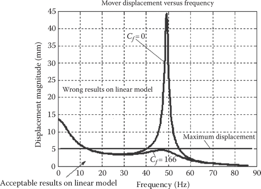
FIGURE 17.30 Magnitude displacement frequency response. (After Tutelea, L. et al., IEEE Trans., IE-55(2), 492, 2008.)

The loading friction coefficient, c_f = 166, was chosen to produce the maximum mechanical power at mechanical resonance frequency. The voltage magnitude V₁ = 180 V was chosen to keep the displacement magnitude closer and under its maximum value of 5 mm for loading conditions, Figure 17.30. For this voltage, the no-load displacement is very large. In fact, for the real machine, the maximum mechanical available displacement is 8 mm and the force is changing sign at 5 mm. The linear model is approximately correct only for mover displacements smaller than 5 mm. However, the model shows that it is necessary to reduce the voltage magnitude about nine times for the no-load regime.

The mechanical power (for harmonic oscillation) is

P_{m e c} = \frac{1}{2} c_{f} {(ω X_{m})}^{2} (17.65)

$P_{m e c} = \frac{1}{2} c_{f} {(ω X_{m})}^{2} (17.65)$

The mechanical power reaches its maximum at electromechanical resonance frequency (Figure 17.31), while the maximum efficiency reaches its maximum value around the mechanical resonant frequency (Figure 17.32).

The current and mover speed are in phase at mechanical resonance frequency as shown in Figure 17.33. The current phase, considering the voltage phase as reference, changes from a large negative value to a large positive value when the electrical frequency passes through the mechanical resonant frequency, for no-load regime. The mechanical and electromechanical resonance frequencies are points of extreme for machine behavior. The machine features are totally different at these frequencies as it is shown in Figure 17.34, for current versus load coefficient, and, respectively, in Figure 17.35, for the mover displacement versus load coefficient.

The efficiency versus output power at constant frequency (mechanical, respectively, electromechanical resonance frequency) is shown in Figure 17.36. The curves in solid line are for displacement smaller than 5 mm, and only these points could be obtained with the real machine. The efficiency is computed considering only the copper losses.

17.3.3.2 FEM Analysis

The parameters of the state-space model of the linear oscillatory machine could be determined by tests on an existing machine, but this procedure does not work during the design process. The FEM analysis could be used for this scope. The FEM setup and magnetic field lines are shown in Figure 17.37 for the interior PM flux concentration linear oscillatory machine (Figure 17.27b). Moreover, the FEM analysis could provide a piece of information otherwise difficult to measure: the airgap flux density shown in Figure 17.38. The FEM analysis is validated by the measured thrust (Figure 17.39) and inductance (Figure 17.40).

Images

FIGURE 17.31 Output power at constant load coefficient. (After Tutelea, L. et al., IEEE Trans., IE-55(2), 492, 2008.)

Images

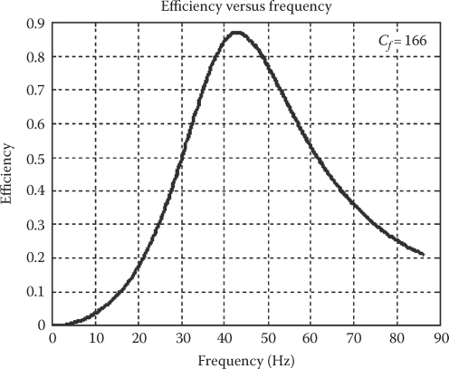
FIGURE 17.32 Efficiency at constant load coefficient. (After Tutelea, L. et al., IEEE Trans., IE-55(2), 492, 2008.)

The FEM results are in good agreement with standstill tests, as shown in Figure 17.39.

The FEM inductance does not contain the overhang leakage inductance, so it is below the measured inductance with about 20 mH. Also for small current, the FEM inductance is constant compared with measured inductance. The core magnetic saturation curve is linearized around zero current in order to improve the algorithm convergence. The agreement between FEM and test results is satisfactory, considering the measurement errors. The FEM analysis could produce the parameters for the linear state model and also for the nonlinear model via look-up tables.

Images

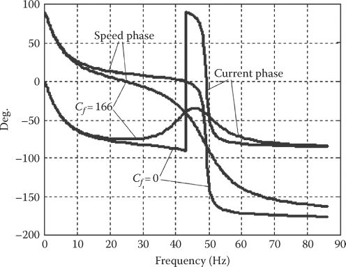
FIGURE 17.33 Current and speed phase versus frequency. (After Tutelea, L. et al., IEEE Trans., IE-55(2), 492, 2008.)

Images

FIGURE 17.34 Current versus loading coefficient. (After Tutelea, L. et al., IEEE Trans., IE-55(2), 492, 2008.)

17.3.3.3 Nonlinear Model

The nonlinearities are produced by the dependence of flux derivative on position and by magnetic saturation and cogging force.

The permanent magnet flux derivative depends on the mover position and could be available in the model via a table. A trapezoidal shape may be considered, as shown in Figure 17.41.

The cogging force dependence on the mover position is introduced in the MATLAB-Simulink model also as a look-up table from test results, after noise filtering (Figure 17.42).

The friction force could be divided into viscous friction force F_vf and Coulomb friction force F_Cf, which is the other nonlinearity source, especially in small oscillations around equilibrium position:

F_{f} = F_{C f} + F_{v f}

$F_{f} = F_{C f} + F_{v f}$

Images

FIGURE 17.35 Displacement magnitude versus loading coefficient. (After Tutelea, L. et al., IEEE Trans., IE-55(2), 492, 2008.)

Images

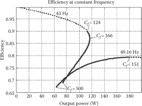
FIGURE 17.36 Efficiency versus output power. (After Tutelea, L. et al., IEEE Trans, IE-55(2), 492, 2008.)

Images

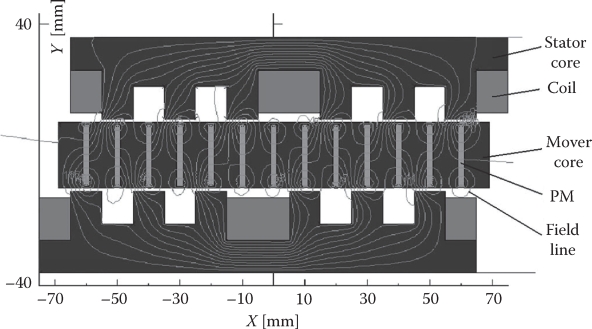
FIGURE 17.37 FEM setup and magnetic field lines for mover at maximum force position and 1 A/coil current. (After Tutelea, L. et al., IEEE Trans, IE-55(2), 492, 2008.)

Images

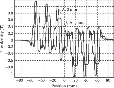
FIGURE 17.38 Air gap flux density by FEM. (After Tutelea, L. et al., IEEE Trans., IE-55(2), 492, 2008.)

Images

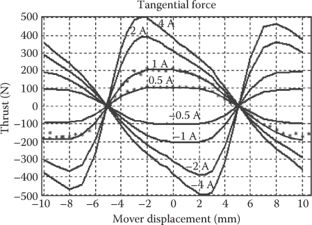
FIGURE 17.39 Thrust versus mover position and coil current; -solid line—FEM simulation, * standstill test. (After Tutelea, L. et al., IEEE Trans., IE-55(2), 492, 2008.)

Images

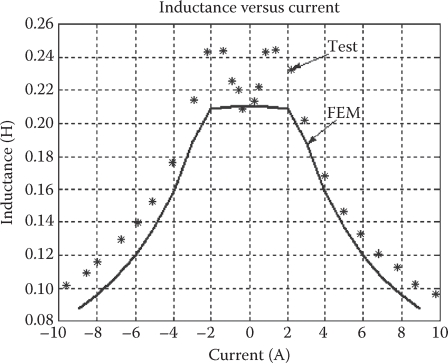
FIGURE 17.40 Machine inductance versus current—two parallel paths. (After Tutelea, L. et al., IEEE Trans., IE-55(2), 492, 2008.)

Images

FIGURE 17.41 Flux derivative distribution. (After Tutelea, L. et al., IEEE Trans, IE-55(2), 492, 2008.)

Images

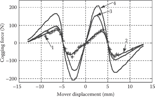
FIGURE 17.42 Cogging force: (1) measured points for FCPM, (2) approx. curves for FCPM, (3) approx. curves for SPM, (4) sum of 2 and 3. (After Tutelea, L. et al., IEEE Trans, IE-55(2), 492, 2008.)

F_{f} = {\begin{array}{l} F_{C} s i g n (u) + k_{v f} u & for u \neq 0 \\ \min (| F_{r e z} |, F_{c}) \cdot s i g n (F_{r e z}) & for u = 0 \end{array} (17.66)

$F_{f} = {\begin{array}{l} F_{C} s i g n (u) + k_{v f} u & for u \neq 0 \\ \min (| F_{r e z} |, F_{c}) \cdot s i g n (F_{r e z}) & for u = 0 \end{array} (17.66)$

where F_rez is the sum of electromagnetic force and mechanical spring force.

The mechanical spring force is assumed to vary linearly with mover displacement, except for the accidental situation when the mover hits the frame, or the spring is fully compressed, when the elastic force suddenly increases.

Finally, the nonlinear model of the linear machine is shown in Figure 17.43, considering constant parameters as R, coil resistance; L, coil inductance; k_f, force coefficient (maximum value of flux derivative versus position); m, mover mass; k_s, spring constant; F_c, Coulombian friction force; c_f, viscous friction coefficient; and x_max, maximum mechanical stroke. Moreover, the model contains two distributions: flux derivative versus position and cogging force versus position already presented in Figures 17.41 and 17.42, respectively. Core losses have been neglected.

Images

FIGURE 17.43 Block diagram of the linear machine nonlinear model. (After Tutelea, L. et al., IEEE Trans., IE-55(2), 492, 2008.)

The force coefficient and, respectively, the inductance dependence on current cannot be neglected when the linear oscillatory machine is working in heavy magnetic saturation conditions, as in our prototype for a large output power. The look-up table method could also be used in this case. The force coefficient is

K_{f} (i, x) = k_{i f} (i) \cdot k_{x f} (x) (17.67)

$K_{f} (i, x) = k_{i f} (i) \cdot k_{x f} (x) (17.67)$

The force coefficient dependence on current (from FEM), k_if, is shown in Figure 17.44, while the force dependence coefficient versus mover displacement k_xf has the same variation as was shown in Figure 17.41, except for the magnitude that is unity.

Images

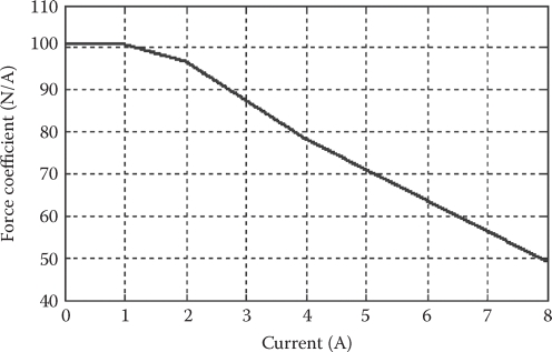
FIGURE 17.44 Force coefficient versus current. (After Tutelea, L. et al., IEEE Trans., IE-55(2), 492, 2008.)

Images

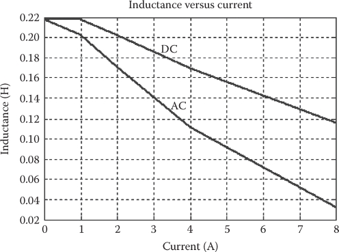
FIGURE 17.45 DC and AC inductance versus current. (After Tutelea, L. et al., IEEE Trans, IE-55(2), 492, 2008.)

The ac inductance, computed from FEM results (17.68), is used in the look-up table and it is shown in Figure 17.45:

\begin{array}{l} L_{a c k} = \frac{Ψ (I_{k + 1}) - Ψ (I_{k})}{(I_{k + 1}) - I_{k}} + 0.02 \\ I_{a k} = \frac{I_{k + 1} + I_{k}}{2} \end{array} (17.68)

$\begin{array}{l} L_{a c k} = \frac{Ψ (I_{k + 1}) - Ψ (I_{k})}{(I_{k + 1}) - I_{k}} + 0.02 \\ I_{a k} = \frac{I_{k + 1} + I_{k}}{2} \end{array} (17.68)$

where the 0.02 H term is the end coil leakage inductance.

The block diagram of the nonlinear model, considering the force coefficient and inductance dependence on current, is shown in Figure 17.46. A larger current was observed in the test results than in the simulation results. This is produced by a construction particularity, as a screw bolt was used to tighten the lamination core. The effect of this equivalent short-circuited cage was observed also in the dc decay standstill tests, when the current did not fall along a single exponential wave. In addition, the force versus current hodograph had a loop when it was acquired in standstill tests at low frequency (1 Hz) ac current. The cage introduced in this particular construction is increasing the current and is producing the additional voltage drop on the coil resistance and inductance leakage.

Images

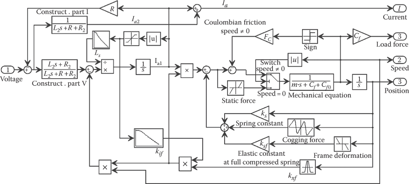
FIGURE 17.46 Block diagram considering inductance and force coefficient dependence on current. (After Tutelea, L. et al., IEEE Trans, IE-55(2), 492, 2008.)

The parameters of equivalent cage L₂ = 0.35 H and R₂ = 40 Ω were chosen in order to minimize the simulation current and efficiency error related to test values for several load points (45-230 W output power). Constant parameters of the equivalent cage when the main inductance has large variations is a compromise and thus the simulation results do not fit closely the test results; however, they are better than in the case of other models. A comparison of results produced with different models and tests is shown in Figure 17.47, voltage magnitude versus mechanical output power; Figure 17.48, current magnitude; and Figure 17.49, efficiency, where the curve 1 represents the test results, curve 2 the simulations on nonlinear model considering the prototype construction particularity, curve 3 the simulations on nonlinear model, and curve 4 the simulations on linear model. The efficiency could increase by around 15%–20% by eliminating the construction problem.

Images

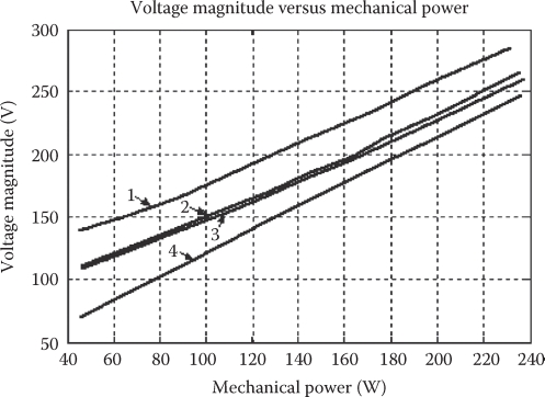
FIGURE 17.47 Supplied voltage: (1) test results, (2) simulation on nonlinear model considering construction particularity, (3) simulation on nonlinear model, and (4) simulation on linear model. (After Tutelea, L. et al., IEEE Trans., IE-55(2), 492, 2008.)

Images

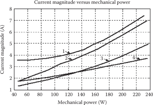
FIGURE 17.48 Current: (1) test results, (2) simulation on nonlinear model considering construction particularity, (3) simulation on nonlinear model, and (4) simulation on linear model. (After Tutelea, L. et al., IEEE Trans, IE-55(2), 492, 2008.)

Images

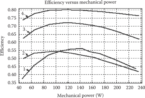
FIGURE 17.49 Efficiency: (1) test results, (2) simulation on nonlinear model considering construction particularity, (3) simulation on nonlinear model, and (4) simulation on linear model. (After Tutelea, L. et al., IEEE Trans., IE-55(2), 492, 2008.)

Images

FIGURE 17.50 Current and position waves. (After Tutelea, L. et al., IEEE Trans., IE-55(2), 492, 2008.)

The current and position waves in dynamic simulation and test results are shown in Figure 17.50.

The simulation base times were shifted to overlap the simulation position and measured position. The current-speed (position) phase is very sensitive to frequency around the resonance frequency (Figure 17.33), so a small error in the model parameters (resonance frequency) could produce a large error in the current-speed phase. Moreover, it is the short-circuit cage, which was not fully modeled and which should be eliminated in a future prototype.

Free deceleration of back-to-back coupled machines simulation is in good agreement with test results (Figure 17.51).

17.3.3.4 Parameters Estimation

Some of the model parameters, such as the resistance, could be measured directly while the inductance is computed from dc current decay tests and the flux derivative with mover position is computed from standstill thrust measurement.

Images

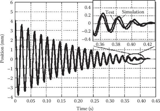
FIGURE 17.51 Free oscillation test and simulation for coupled machines particularity (short-circuit cage). (After Tutelea, L. et al., IEEE Trans, IE-55(2), 492, 2008.)

TABLE 17.3
Machine Parameters

Images

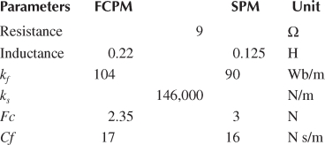
Free oscillation of mover during free deceleration test was recorded to find the mechanical resonance frequency for each machine and also for the two machines, when mechanically coupled back to back as in dynamic tests. The Coulomb friction force, F_c, and viscous coefficient, C_f, are adjusted in order to produce the same mover displacement in the simulation as in recorded data that were measured by a laser-based position transducer. The machine parameters are shown in Table 17.3.

17.3.3.5 Further Performance Improvements

The FEM results on thrust and inductance are in good agreement with the test results. Therefore, we conclude that we can use the FEM to design a better oscillatory machine. By reducing the airgap from 1 to 0.4 mm, and by increasing the PM height from 2 to 3 mm and the stator back core from 10 to 15 mm, the airgap flux density is increased (Figure 17.52) due to real flux concentration. Consequently, the thrust versus current is increased more than three times as it is observed in Figure 17.53. The inductance does not increase much (Figure 17.54), so the voltage drop on it does not increase notably. In conclusion, the power density and efficiency could be dramatically improved.

Note: This paragraph, starting from experiments, is indicative of the various problems encountered in modeling an LOM to fit test results.

Images

FIGURE 17.52 Airgap flux density on improved design. (After Tutelea, L. et al., IEEE Trans., IE-55(2), 492, 2008.)

Images

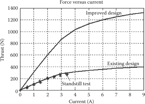
FIGURE 17.53 Thrust for existing and improved designs. Solid line- FEM, * standstill test, 2 parallel path. (After Tutelea, L. et al., IEEE Trans, IE-55(2), 492, 2008.)

Images

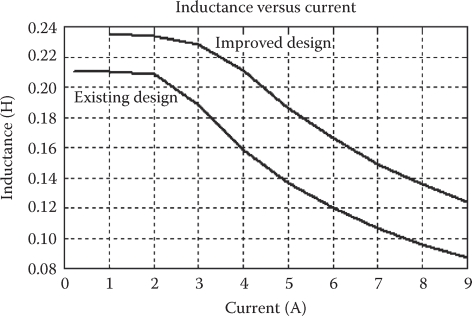
FIGURE 17.54 Inductance for existing and improved design, FEM at zero mover displacement. (After Tutelea, L. et al., IEEE Trans, IE-55(2), 492, 2008.)

17.4 Iron-Mover Stator PM LOMs

Aside from the iron-mover stator PM LOM, presented in the chapter on “plunger solenoids,” two typical tubular and one flat double-sided LOMs are shown in Figure 17.55.

As the flux-switching topology (Figure 17.55a) was already investigated in a slightly different shape in the “Plunger Solenoids” chapter, and the tubular flux is referred to in [8], only the configuration in Figure 17.55c is briefly discussed here.

It may be called a “flux-switching” topology, but this is the same as “flux reversal.” Figure 17.55c illustrates a longitudinal flux topology, but a transverse flux one may also be feasible in a single-sided configuration. However, the net ideally zero normal force of a double-sided configuration is paramount in easing the task of the linear bearings (or mechanical flexures) used to “guide” the linear motion.

Together with other iron-mover LOMs, the flat FR stator PM configuration shows a few peculiarities such as the following:

The iron mover tends to be heavier than the coil mover or the PM mover for the same thrust, stroke, and frequency.
The airgap variations lead to notably uncompensated normal force (due to the small airgap).
There is a strong cogging force, which in general may not be used as a “magnetic” spring due to its insufficient level and “wrong” direction.
The rather large inductance leads to lower power factor, slower current response, and stronger danger of PM demagnetization.
Fringing and leakage PM flux are important, and optimal geometrical design should be used to reduce them.
The force (and emf) coefficient K_e(x) depends notably on mover position, so the emf departs from a sinusoidal waveform and so does the current for sinusoidal input voltage; all this might lead to some vibration and noise.

Images

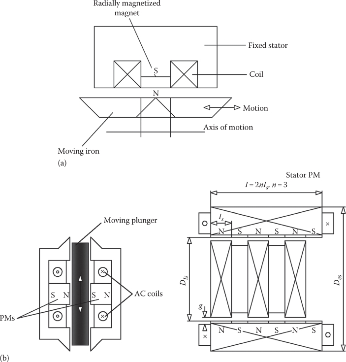
FIGURE 17.55 Iron-mover stator PM LOM(G)s (a) tubular with pulsed-PM flux, (b) tubular with flux reversal, (c) flat with PM flux concentration (double sided). (After Redlich, R.W. and Berchowitz, D.H., Proc Inst. Mech. Eng, 199(3), 203, 1985.)

Images

17.5 Linear Oscillatory Generator Control

LOGs driven by a spark-ignited gasoline linear engine or by a Stirling free-piston engine may operate stably in stand-alone mode based on the prime mover stabilizing means.

For small powers, a Stirling free-piston engine may, by its controller, function stably at the power grid and deliver controlled power at the grid frequency [15–18].

Reference [15] introduces a model for the two-cylinder internal combustion linear engine (ICLE) by using the balance of forces:

P_{L} (x) A_{b} - P_{R} (x) - F (x) = m_{t} \ddot{x} (17.69)

$P_{L} (x) A_{b} - P_{R} (x) - F (x) = m_{t} \ddot{x} (17.69)$

P_L is the instantaneous pressure in the left cylinder

P_R is the instantaneous pressure in the right cylinder

A_b is the bore area

F(x) is the electromagnetic (LOG) force and mechanical (spring, if any) force m_t is the total mover mass

Under no-load and ideal (frictionless) conditions, no spring is required to sustain the mover motion: gas compressing and expending forces will do it, and thus, the natural frequency of the engine is reached.

In the absence of mechanical springs and of cogging force, the force balance of ICLE, at no load, can be written [16,17]

A_{B} P_{1} {(\frac{2 r}{r + 1})}^{n} [{(1 + \frac{x}{x_{n}})}^{- n} - {(1 - \frac{x}{x_{m}})}^{- n}] = m_{t} \ddot{x} (17.70)

$A_{B} P_{1} {(\frac{2 r}{r + 1})}^{n} [{(1 + \frac{x}{x_{n}})}^{- n} - {(1 - \frac{x}{x_{m}})}^{- n}] = m_{t} \ddot{x} (17.70)$

P₁ is the intake pressure

x_m = l_stroke/2 is the mid position of mover

r is the combustion ratio

n is a constant

Equation 17.70 leads to a close to harmonic motion (under no load). As during load and in real conditions (nonzero friction and cogging force) the motion frequency is slightly reduced, the introduction of a mechanical spring may bring back the no-load resonance frequency conditions.

For a Stirling engine linear force piston prime mover (Figure 17.56a), a stability analysis was performed in [18,19]. Stability means damped oscillations. For this the Stirling engine displacer and power pistons, the electric current, and the emf must have the grid frequency ω. Stability is based on the inequality

W_{d} \leq W_{c} (17.71)

$W_{d} \leq W_{c} (17.71)$

where W_c is the total energy removed from the shaft (by the LOG) over one cycle of ω:

W_{c} = P_{c} \frac{2 π}{ω} (17.72)

$W_{c} = P_{c} \frac{2 π}{ω} (17.72)$

and W_d is energy generated over one cycle of ω (by the Stirling engine)

W_{d} = P_{d} \frac{2 π}{ω} (17.73)

$W_{d} = P_{d} \frac{2 π}{ω} (17.73)$

A typical result for a Stirling engine and an LOG with a series capacitor C_s is shown in Figure 17.56b [19]. For a few output power levels (2, 10, 20, 25, 30 kW), stability gradually grows from 55–60 to (55–71) Hz frequencies.

A trade-off between a stronger PM and a larger tuning capacitor C_s, based on minimum initial cost, may be performed.

The tuning capacitor C_s does a few things:

Increases the rate of power removal from the prime mover P_c, such that it is faster than the rate of power generated by the engine, P_d.
It may reduce the danger of PM demagnetization during larger loads; not so under sudden short circuit.
Improves the LOG power factor.

All three requirements are important, but the first two demand higher priority in sizing the tuning capacitor. An additional mechanical spring would change the picture of stability mostly for the better, but the resonance frequency may be more rigid, to follow and secure maxim LOG efficiency.

Images

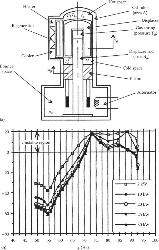
FIGURE 17.56 (a) Stirling engine linear prime mover and (b) Bode plots stability analysis. (After Tutelea, L. et al., IEEE Trans., IE-55(2), 492, 2008.)

However, if a converter is used, and a strong mechanical spring “governs” the motion, the system may be close-loop stabilized either for grid or for autonomous operation (Figure 17.57).

As expected, the dual converter may operate bidirectionally and under open- or close-loop control, either in generator or in motor mode.

Images

FIGURE 17.57 LOG with bidirectional converter control. (After Redlich, R.W. and Berchowitz, D.H., Proc Inst. Mech. Eng., 199(3), 203, 1985.)

17.6 Lom Control

The control for motoring depends heavily on the application. As operation at resonance is most desirable, only a small adjustment of frequency to produce minimum current would be required.

Also, the larger the voltage, the larger the stroke length for larger load force, in general.

As a strong mechanical spring is used “to control” the motion, the question arises if position close-loop control may be eliminated for applications where its exact matching is not critical. Let us consider reciprocating compressors (Figure 17.58) [20].

The current amplitude versus stroke characteristics at a few frequencies (Figure 17.59) [19] shows that, say at 50 Hz, the stroke increases almost linearly with the amplitude of current after the pumping point (right side in Figure 17.59) is reached.

This should indicate that current control is sufficient and thus, position control for vapor compressors may be eliminated.

A B-spline neural network+PI current controller (Figure 17.60) is shown to produce good results with the phase angle (θ) of the sinusoidal current command as input [19].

Even when the current reference is increased, to increase stroke, the response in current, position, and compressor pressure are all stable (Figure 17.61), after [19].

Images

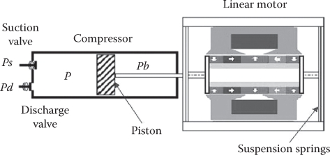
FIGURE 17.58 Linear compressor LOM. (After Boldea, I. and Nasar, S.A., Linear Motion Actuators and Generators, Chapter 8, Cambridge University Press, Cambridge, U.K., 1997.)

Images

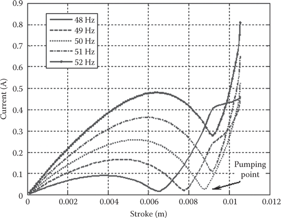
FIGURE 17.59 Current versus l_stroke curves for linear compressor. (After Lim, Z. et al., A hybrid current controller for linear reciprocating vapor compressors, Conference Record of the IEEE Industry Applications Society Annual Meeting (IEEE-IAS’2007), New Orleans, LA, 2007.)

Images

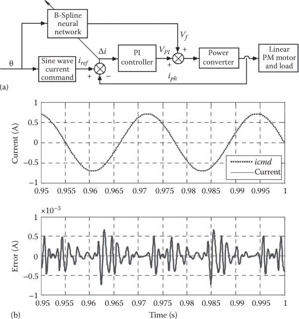
FIGURE 17.60 (a) BSNN current controller for LOM and (b) typical results. (After Lim, Z. et al., A hybrid current controller for linear reciprocating vapor compressors, Conference Record of the IEEE Industry Applications Society Annual Meeting (IEEE-IAS’2007), New Orleans, LA, 2007.)

Images

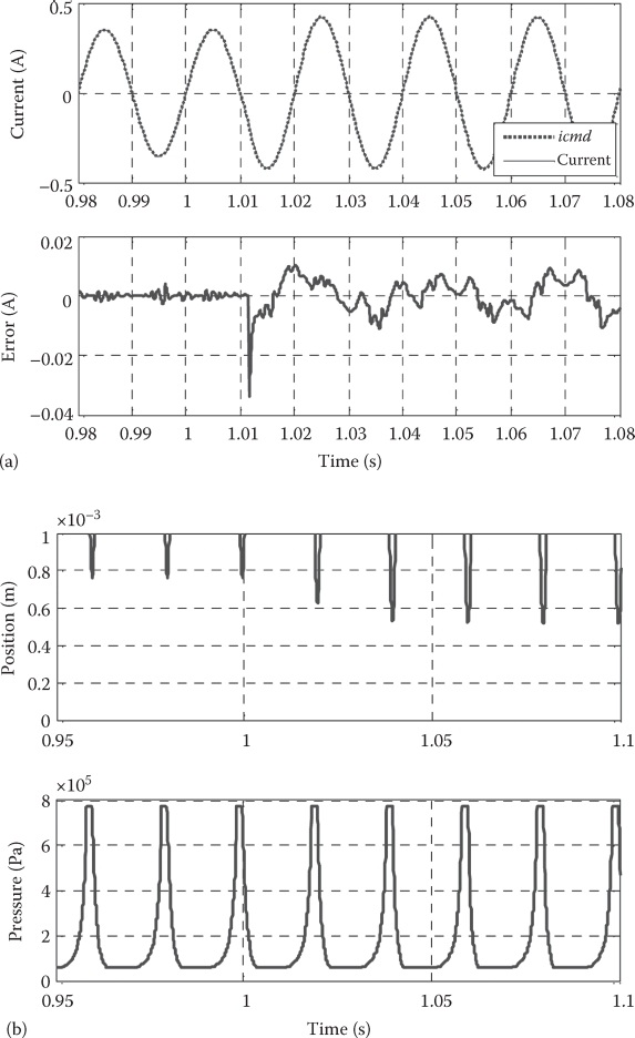
FIGURE 17.61 (a) Current transient response and (b) position and pressure response. (After Lim, Z. et al., A hybrid current controller for linear reciprocating vapor compressors, Conference Record of the IEEE Industry Applications Society Annual Meeting (IEEE-IAS’2007), New Orleans, LA, 2007.)

TABLE 17.4
Prototype of Linear Compressor: Parameters

Supply voltage V (V_rms)	230	Average force constant KTa (N/A)	92
Nominal frequency f (Hz)	50	Motor inductance Le (H)	0.45
Total moving mass m (kg)	0.43	Motor resistance Re (Ω)	02.5
Spring constant K (kN/m)	29.8	Viscous damping B (N s/m)	1.10
Rated stroke U (mm)	10.5

The PI current controller alone was shown incapable of small enough current regulation errors. Typical data of the prototype in [19] are given in Table 17.4.

Other robust current controllers (such as sliding mode + PI) may also apply even for a smaller computation effort, as shown in Chapter 15, dedicated to “plunger solenoids.”

17.7 SUMMARY

Single-phase PM linear oscillatory synchronous motors/generators are preferred for quite a few applications with a stroke of up to 60 mm or so, while operating at constant frequency f1 and variable voltage.
Mechanical spring (for vapor compressor load) or the prime mover (linear internal combustion engine or Stirling engine) is capable of harmonic linear motion at resonance (fm = f₁).
This way the efficiency is high because the electromagnetic force deals only with the load, while the mover motion is controlled mechanically (by the mechanical spring or by the prime mover (for generator mode).
The stroke length l_stroke corresponds to two motion amplitudes x_max (l_stroke = 2x_max):

$x (t) = x_{\max} \sin (2 π f_{1} t); f_{1} = f_{m} (17.74)$ $x (t) = x_{\max} \sin (2 π f_{1} t); f_{1} = f_{m} (17.74)$
The stroke may be assimilated to the electric machine pole pitch τ; consequently, when the load decreases, the stroke (pole pitch) is reduced by reducing the voltage at resonance frequency f₁ =f_m. So at reduced loads the excursion length and speed are reduced by reducing a “virtual” pole pitch in the single-phase PM linear synchronous machine; but modifying pole pitch is, in terms of efficiency, as good as modifying frequency to reduce speed; this explains why the efficiency at reduced loads remains large. This is a special merit of LOM(s).
There are tubular [9] and flat topologies [21–23] for LOM(G)s; the tubular ones enjoy “the blessing” of circularity and thus show ideally zero radial (normal) force and, consequently, the mechanical flexures (or linear bearings) are “saved” very large normal forces; for flat structures, double-sided configurations are required to preserve this asset.
The heavier the mover of LOM(G)s, the larger the mechanical spring for given eigen-frequency f_m =f₁; air-coil movers and PM movers tend to result in lower mover weight and thus imply smaller (less expensive) mechanical springs, but they are mechanically more fragile as their framing should be nonmagnetic with low electrical conductivity (siluminum, Kevlar, etc.)

There are also iron movers to consider, though their weight tends to be larger for given stroke, frequency, and power, but they are rugged mechanically and the PMs on the stator are better protected mechanically and thermally.
The coil movers require a mechanically flexible electric power cable, which might be a liability for some applications.
As even a small departure from resonance frequency leads to notable reduction in LOM(G) efficiency, operation with an inverter, to trace minimum current in correcting the reference frequency, is required.
LOM(G)s lack the rotary to linear mechanical transmission and could compete with standard rotary motor drives for LOMs if their efficiency is high and their total cost is competitive at equal or better reliability, which is the case with PM LOM(G)s.
Air-coil-mover LOMs may be built in the tenth of kW range for, say, series hybrid electric vehicle generators driven by dual linear piston gas engines, and down to small powers in microspeakers (or recorders for mobile phones, etc.).

The coil in air with surface PMs on the stator leads to a small electric time constant, which provides acceptable power factor at large powers and fast current (force) response in low-power applications.
A 20 kW, 60 mm stroke, 60 Hz LOG is proven to show 90% efficiency at 0.8 lagging power factor in a 110 kg stator and 30 kg mover device (average speed is only 3.6 m/s, which explains the not so small weight/kW).
For microspeakers/receivers with high-quality sound and broad frequency range (kHz), reduced size and cost are paramount; radiated sound power, dependent on linear speed, geometry, etc., are related to sound pressure level (SPL); harmonic distortion, then, defines the sound quality globally.

Once the diaphragm speed is given, the integration of microspeaker and dynamic receiver LOM(G), with PM flux concentration, was proven to produce competitive performance in a smaller volume device.

To avoid the necessity of a mechanically flexible electric power cable, the PM-mover topologies have been introduced, especially for vapor compressors.
The tubular homopolar PM-mover, single-coil, C-core stator topology, first introduced by Redlich in the 1980s has become commercial, and others with multiple heteropolar PM mover and multiple-coil stators have been proposed in the last two decades.
The tubular homopolar PM mover (Redlich) topology, though it leads to a moderate airgap PM flux density, overall leads to a low-weight device of pancake shape with a good efficiency.
The multiple heteropolar PM mover with multiple stator topology is proven in this chapter to produce 25 W at 270 Hz, 6 mm stroke at 74% efficiency within a device whose total weight is around 60 g (mover weight: 16 g). An increase in size would jump the efficiency to 80%–85%; a two-pole PM-mover device was proven to produce 42 W at 89% efficiency for a 10 mm stroke at 50 Hz, however, for 866 g total weight (230 g mover), which demands a strong (large) mechanical spring [24].
A double-sided flat flux-reversal LOM is introduced and analyzed in detail with experiments to illustrate various techniques in its characterization; PM flux concentration in the mover is performed to increase force/total weight and efficiency, but the PM flux concentration leads to a high p.u. inductance and thus moderate power factor (limited frequency).
Iron-mover LOMs have rugged movers but suffer from high inductance p.u. syndrome; they are suitable when safety (reliability) is critical for a long life (such as in vapor compressors, Stirling engine driven LOGs for deep space missions).
LOGs may produce sustained harmonic motion by the prime mover, even without mechanical springs, by using wisely a centralizing large linear cogging force obtained by expert design [11].
Both a two-piston linear ICE and the Stirling (free-piston) engine have been proven capable of stable motion; mechanical springs may be added to help stability and so is a tuning series capacitor in the LOG.
The ultimate control of LOGs (and LOMs) is close-loop control, which needs, for bidirectional power flow, a dual (back to back) inverter.
For LOM, the control depends on the application; for vapor compressors, the robust current control was proved sufficient (no position control is needed), beyond the pumping point of the compressor.
Overall, resonance single-phase PM linear motors/generators prove to be highly competitive devices for applications with strokes from under 1 to 60 mm (or so) and stroke length at frequencies from 40-60 to 300 Hz and more (at very low power). Strong R&D and industrial efforts are expected with LOM(G)s, especially for vapor compressors [20,22], Stirling engine generators, and microspeakers/dynamic receivers.

References

1. I. Boldea and S.A. Nasar, Linear Electromagnetic Devices, Chapter 7, Taylor & Francis Group, New York, 2001.

2. S.M. Hwang, H.J. Lee, K.S. Hong, B.S. Kang, and G.Y. Hwang, New development of combined PM type microspeakers used for cellular phones, IEEE Trans., MAG-41(5), 2005, 2000–2003.

3. S.M. Hwang, K.S. Hong, H.J. Lee, J.H. Kim, and S.K. Jeung, Reduction of dynamic distortion in dual magnetic type microspeakers, IEEE Trans., 40(4), 2004, 3054–3056.

4. S.M. Hwang, H.J. Lee, J.H. Kim, G.Y. Hwang, W.Y. Lee, and B.S. Kang, New developments of integrated microspeakers and dynamic receivers used for cellular phones, IEEE Trans, MAG-39(5), 2003, 3259–3261.

5. F.F. Mazda, Electronic Instruments and Measurement Techniques, Cambridge University Press, Cambridge, U.K., 1987.

6. T. Mizuno, M. Kaway, F. Tsuchiya, M. Kosugi, and H. Yamada, An examination for increasing the motor constant of a cylindrical moving magnet-type linear actuator, IEEE Trans., MAG-41(10), 2005, 3976–3978.

7. J. Wang, D. Howe, and Z. Lin, Comparative study of winding configurations of short-stroke, single phase tubular permanent magnet motor for refrigeration applications, Conference Record of the IEEE Industry Applications Society Annual Meeting (IEEE-IAS’2007), New Orleans, LA, 2007.

8. R.W. Redlich and D.H. Berchowitz, Linear dynamics of free piston Stirling engine, Proc. Inst. Mech. Eng, March 1985, 199(3), 203–213.

9. T. Ibrahim, J. Wang, and D. Howe, Analysis of a short-stroke, single-phase tubular PM actuator for reciprocating compressors, International Symposium on Linear Drives for Industrial Applications (LDIA2007), Lillie, France, 2007.

10. I. Boldea, Variable Speed Generators, Chapter 12, CRC-Press, Taylor & Francis Group, New York, 2006.

11. I. Boldea, S. Agarlita, and L. Tutelea, Springless resonant linear oscillatory PM motors? International Symposium on Linear Drives for Industrial Applications (LDIA2011), Eindhoven, the Netherlands, 2011.

12. C. Pompermaier, F.J. Kalluf, M.V. Ferreira da Luz, and M. Sadowski, Analytical and 3D FEM modeling of a tubular linear motor taking into account radial forces due to eccentricity, IEEE International Electric Machines and Drives Conference (IEMDC’09), Miami, FL, 2009.

13. L. Tutelea, M.Ch. Kim, M. Topor, J. Lee, and I. Boldea, Linear PM oscillatory machine: Comprehensive modeling for transients with validation by experiments, IEEE Trans., IE-55(2), 2008, 492–500.

14. L. Tutelea, M.C. Kim, T.H. Kim, J. Lee, and I. Boldea, Development of a flux concentration type linear oscillatory machine, IEEE Trans., MAG-40(4), 2004, 2092–2094.

15. C. Pompermaier, K.F.J. Haddad, A. Zambonetti, M.V. Ferreira da Luz, and I. Boldea, Small linear PM oscillatory motor: Magnetic circuit modeling corrected by axisymmetric 2-D FEM and experimental characterization, IEEE Trans., IE-59(3), 2012, 1389–1396.

16. N. Clark, S. Nandkumar, and P. Famouri, Fundamental analysis of a linear two-cylinder ICE, Record of SAE International FUEL and Lubricants Meeting and Exposition, San Francisco, CA, 1998.

17. A. Cosic, I. Lindback, W.M. Arshad, and P. Thelis, Application of a free-piston generator in a series hybrid vehicle, Proceedings of the Fourth International Symposium on Linear Drives for Industry Applications (LDIA’2003), Birmingham, U.K., 2003, pp. 541–544.

18. Z.X. Fu, S.A. Nasar, and M. Rosswurm, Stability analysis of free piston Stirling engine power generation system, 27th IECECE Conference, San Diego, CA, August 3–7, 1992.

19. I. Boldea and S.A. Nasar, Linear Motion Actuators and Generators, Chapter 8, Cambridge University Press, Cambridge, U.K., 1997.

20. Z. Lim, J. Wang, and D. Howe, A hybrid current controller for linear reciprocating vapor compressors, Conference Record of the IEEE Industry Applications Society Annual Meeting (IEEE-IAS’2007), New Orleans, LA, 2007.

21. I. Boldea, S.A. Nasar, B. Penswich, B. Ross, and R. Olan, New linear reciprocating machine with stationary PM, Conference Record of the IEEE Industry Applications Society Annual Meeting (IEEE-IAS’1996), New Orleans, LA, 1996, vol. 2, pp. 825–829.

22. J. Lee and I. Boldea, Linear reciprocating flux reversal PM machine, US patent No. 6538.349, 25.03. 2003

23. L. Tutelea, M.C. Kim, T.M. Kim, J. Lee, and I. Boldea, A set of experiments to more fully characterize linear PM oscillatory machines, IEEE Trans., MAG-41(10), 2005, 4009–4011.

24. Z.Q. Zhu and X. Chen, Analysis of an E-core interior PM linear oscillating actuator, IEEE Trans., MAG-45(10), 2009, 4384–4387.

..................Content has been hidden....................

You can't read the all page of ebook, please click here login for view all page.

Table of Contents for
Chapter 17 Resonant Linear Oscillatory Single-Phase PM Motors/Generators

17 Resonant Linear Oscillatory Single-Phase PM Motors/Generators

17.1 Introduction

17.2 Coil-Mover LOMs (LOGs)

17.2.1 Four-Coil-Mover LOM: Modeling and Design by Example

17.2.1.1 Airgap: PM Flux Density

17.2.1.1.1 Airgap Diameter D_iPM and PM Length l_PM

17.2.1.2 Inductance

17.2.1.3 Core Sizing and Core Losses

17.2.1.4 The Phasor Diagram

17.2.1.5 The Number of Turns per Coil n_c

17.2.2 Integrated Microspeakers and Receivers

17.3 PM-MOVER LOM(G)

17.3.1 Tubular Homopolar LOM(G)

17.3.2 25 W, 270 Hz, Tubular Multi-PM-Mover Multi-Coil LOM: Analysis by Example

17.3.2.1 General Design Aspects

17.3.2.2 Optimization Methodology by Example

17.3.2.3 FEM Analysis

17.3.2.4 Simplified Linear Circuit Model for Steady State and Transients

17.3.2.5 Nonlinear Circuit Model and MATLAB® Code with Digital Simulation Results

17.3.3 Double-Sided Flat PM-Mover LOM

17.3.3.1 State-Space Model of the Linear Machine

17.3.3.2 FEM Analysis

17.3.3.3 Nonlinear Model

17.3.3.4 Parameters Estimation

17.3.3.5 Further Performance Improvements

17.4 Iron-Mover Stator PM LOMs

17.5 Linear Oscillatory Generator Control

17.6 Lom Control

17.7 SUMMARY

References

Table of Contents for Chapter 17 Resonant Linear Oscillatory Single-Phase PM Motors/Generators

Create new playlist

Sign In

Sign Up

17.2.1.1.1 Airgap Diameter DiPM and PM Length lPM

Table of Contents for
Chapter 17 Resonant Linear Oscillatory Single-Phase PM Motors/Generators

17.2.1.1.1 Airgap Diameter D_iPM and PM Length l_PM