Chapter 19 Attraction Force (Electromagnetic) Levitation Systems

Search in book...
Toggle Font Controls
Create new playlist

Name your new playlist

Playlist description (optional)
Sign In

Email address

Password

Forgot Password?

or

Continue with Facebook

Continue with Google
Sign Up

Full Name

Email address

Confirm Email Address

Password

or

Continue with Facebook

Continue with Google

Attraction levitation systems (ALS) use attraction current–controlled electromagnetic force to control the airgap between fix and mobile mild magnetic cores. Applications for ALS range from magnetic bearings and vibrating tables to magnetically levitated vehicles (MAGLEVs) [1–3].

For MAGLEVs, the primary is placed on board and contains permanent magnet (PM)-less or PM-assisted dc controlled current electromagnets (solenoids) and a solid mild iron fix secondary (track).

On the other hand, for active magnetic bearings and for vibrating tables, the secondary is the mover and is made, in general, from a laminated mild steel core or of a soft magnetic composite (SMC).

In this chapter, we will concentrate on ALS for MAGLEVs, as active magnetic bearing (or bearing-less rotary electric motor) is a field of R&D in itself that deserves a separate treatment.

The following main aspects of ALS for MAGLEVs are treated in what follows:

Competitive topologies
Simplified analytical model (with no end effect) for design
End effect analytical modeling
ALS design methodology and sample performance for MAGLEVs
ALS circuit model for dynamics and control
Open-loop transfer functions of the linearized system
State-space feedback control
Linear parameter varying control
Sliding mode control
Zero power control
Control system performance by example
Collision avoidance
Average control power
Ride comfort

19.1 Competitive Topologies

The most obvious topology of ALS for MAGLEVs comprises C-core (laminated) electromagnets on board of vehicle and C-core (made of solid mild steel) of secondary (track)—Figure 19.1.

The two C-cores of same width L_w allow for a self-centering guidance force when the C-core electromagnets are off-centric; this effect may help the guidance system, which may also be performed with C-core electromagnets.

PMs may be added to the dc controlled electromagnets either in the C-core (Figure 19.2a) or in an Ê-core configuration with dual airgap (Figure 19.2b). Also, the double C-core structure leads to lower eddy currents in the solid iron secondary during vehicle motion and controlled dynamics.

Images

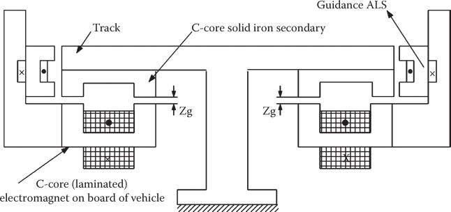
FIGURE 19.1 C-core ALS for MAGLEVs.

Images

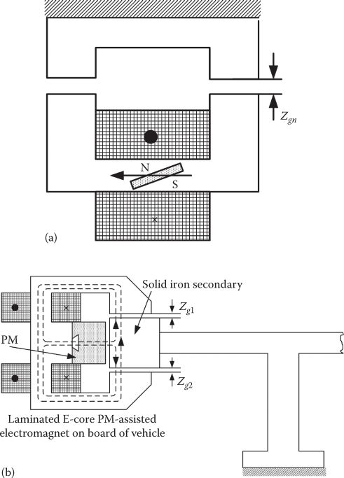
FIGURE 19.2 PM-assisted typical ALS: (a) C-core electromagnet and (b) E-core dual electromagnet.

The PM may be designed to provide for rated airgap Z_gn the entire weight of the vehicle (loaded), with the coil current control used for dynamics and control purposes.

In the E-core topology (Figure 19.2), the two twin coils may be potentially controlled together for levitation control only, or separately if both levitation and guidance control is necessary. Rotated by 90°, the configuration in Figure 19.2b may be used for axial active magnetic bearings also.

As the cost of PMs tends to be high and they experience large (or fast) magnetic flux variations, notable eddy currents are induced in them, apparently their use for MAGLEVs may not be the first choice, despite a drastic reduction in control power.

The solid iron secondary core, chosen for economic reasons, leads to eddy currents induced in it due to

Magnetic flux variation during airgap dynamic control (control eddy currents)
Longitudinal end effect at medium and high speeds of vehicle (end effect eddy currents)

In general, however, for MAGLEVs, the frequency band of ALS is less than 25 Hz. Thus, the control eddy currents should not be very large, but, in active magnetic bearings, the frequency band is notably larger and, thus, they should be accounted for.

On the other hand, the end effect eddy currents are related to the limited length of dc electromagnets traveling at a speed U with respect to the solid core secondary track [4–7].

It is a kind of dc linear eddy current brake in the sense that eddy currents are induced at the entry and exit ends; they decay over a certain length. If the speed is large, the decay length may be a good part of the electromagnet length and thus notable flux density and normal (attraction) force F_n reduction occurs. The eddy currents induced by motion also produce a drag force F_d; the drag force has to be accounted for in the propulsion system design for high speeds.

We will first develop a simplified analytical field model without eddy currents and then treat the latter in a subsequent paragraph.

19.2 Simplified Analytical Model

As the core width b_i=40–60 (80) mm and the airgap Z_g in the MAGLEVs vary from 15 (20) to 8 (10) mm, respectively, in general in interurban and urban applications, the fringing flux (Figure 19.3) has to be considered.

Approximately, the distribution of airgap flux density in the airgap B(z) varies as

B (y) = B 0; for 0 \leq | y | \leq b i 2 (19.1)

$B (y) = B_{0}; for 0 \leq | y | \leq \frac{b_{i}}{2} (19.1)$

B (y) = B 0 \cdot exp ⎛ ⎝ ⎜ - 2 ( | z | - b i 2 ) g 0 ⎞ ⎠ ⎟; for | y | \geq b i 2

$B (y) = B_{0} \cdot \exp (\frac{- 2 (| z | - \frac{b_{i}}{2})}{g_{0}}); for | y | \geq \frac{b_{i}}{2}$

Images

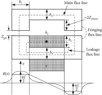
FIGURE 19.3 Airgap distribution along 0y (transverse) axis.

So the average track core flux density B_c is

B c ≅ B 0 (1 + 2 g 0 b i); B 0 = μ 0 W i 2 g 0 ( 1 + K s ( B a v ) ) (19.2)

$B_{c} ≅ B_{0} (1 + \frac{2 g_{0}}{b_{i}}); B_{0} = \frac{μ_{0} W_{i}}{2 g_{0} (1 + K_{s} (B_{a v}))} (19.2)$

where g₀ is the rated airgap.

In the electromagnet C core, there is also an additional leakage flux density whose average value in the core is B_av:

B a v \approx μ 0 W i 2 b c; b c ≫ 2 g (19.3)

$B_{a v} \approx \frac{μ_{0} W_{i}}{2 b_{c}}; b_{c} ≫ 2 g (19.3)$

Only approximately, and because b_c ≫ 2g, we may consider that the average iron flux density in the electromagnetic core B_iav is (if b_i ≈ b_y1 = b_y2)

B i a v \approx B c + B a v (19.4)

$B_{i a v} \approx B_{c} + B_{a v} (19.4)$

This simplified expression could serve in sizing the core thickness (or width b_i = b_y1 = b_y2).

The attraction levitation force F_L0 is

F L 0 = 2 L B 2 0 ( 1 + 2 g 0 b i ) 2 . b i 2 μ 0 (19.5)

$F_{L 0} = \frac{2 L B_{0}^{2} {(1 + \frac{2 g_{0}}{b_{i}})}^{2} . b_{i}}{2 μ_{0}} (19.5)$

In addition, the electromagnet weight G₀ yields

G 0 = 2 L [(2 (b i + h c) b i + b c b i) γ i + W i J c o m (1 + ( b i + h c ) π 2 L) γ c o] (19.6)

$G_{0} = 2 L [(2 (b_{i} + h_{c}) b_{i} + b_{c} b_{i}) γ_{i} + \frac{W_{i}}{J_{c o m}} (1 + \frac{(b_{i} + h_{c}) π}{2 L}) γ_{c o}] (19.6)$

where

L is the electromagnet length

J_co is the design current density

γi, γ_co are the iron and copper (aluminum sheet) mass densities

With a filling factor K_fill = 0.6−0.7, the aluminum-sheet coil cross section b_ch_c is

b c h c = W i J c o n K f i l l (19.7)

$b_{c} h_{c} = \frac{W_{i}}{J_{c o n} K_{f i l l}} (19.7)$

To account for magnetic saturation, we have to consider Equations 19.2 through 19.4 together with the magnetization curve B(H) of the core, applied for B_iav in the electromagnet and B_c in the core of the track.

Images

FIGURE 19.4 Coil flux linkage Ψ(i, g) and attraction force F_L0 (i, g).

Alternatively, a refined magnetic circuit may be developed for the scope. Typical curves of Ψ_c(i, Z_g) may be obtained (as done for solenoids), together with F_L0 (i, Z_g)—Figure 19.4.

Magnetic saturation influence is small at higher airgap (say at standstill airgap: Z_gmax = 2Z_{g rated}), but it may be important at smaller airgaps (say 0.5Z_{g rated}). In general, during dynamic control of airgap, the latter varies by ±20%–25%, as a compromise between energy consumption and collision avoidance with the track.

The Ψ_c (i,g) and F_L0 (i,g) curve families may be better calculated by finite element method (FEM); 2D (or even 3D) FEM is required for the scope.

Curve fitting Ψ_c (i,g) and F_L0 (i,g) functions by simplified polynomial (or exponential) functions will provide reliable data for dynamics and control studies.

To avoid direct touch between the ALS and the track, a thin nonmagnetic-nonconducting coating is stuck to the electromagnet surface.

A sample approximation is

Ψ c \approx c i - d i 2 a Z g + b + L l i : L l - leakage inductance (19.8)

$\begin{matrix} Ψ_{c} \approx \frac{c i - d i^{2}}{a Z_{g} + b} + L_{l} i : & L_{l} - leakage inductance \end{matrix} (19.8)$

F L 0 = K f \cdot (c i - d i 2 a Z g + b) (19.9)

$F_{L_{0}} = K_{f} \cdot (\frac{c i - d i^{2}}{a Z_{g} + b}) (19.9)$

The voltage and motion equations are added to complete the model:

V = R i + d Ψ c d t; M d Z g d t = - F L 0 + M g g + F e x t (19.10)

$\begin{matrix} V = R i + \frac{d Ψ_{c}}{d t}; & M \frac{d Z_{g}}{d t} = - F_{L_{0}} \end{matrix} + M_{g_{g}} + F_{e x t} (19.10)$

19.3 Analytical Modeling of Longitudinal End Effect

As already mentioned, the limited length (up to 1–1.5 m) electromagnets in motion at speed U, with respect to the solid iron secondary, produce eddy currents in the latter. These eddy currents contribute to a nonuniform airgap flux density in the electromagnet area (0 ≤ x ≤ L) and a drag force F_d. While along the transverse (y) direction—Figure 19.3—the eddy currents are assumed to vary sinusoidally, along the direction of motion the electromagnet mmf and initial airgap flux density is rectangular (Figure 19.5) [6,7].

The airgap should be suddenly increased outside the active zone (0 ≥ x ≥ L) to portray properly the field distributions in the entry and exit zones:

B 0 (x) \approx 0 for x < 0 B 0 (x) = B 0 for 0 \leq x \leq L B 0 (x) \approx 0 for x > L (19.11)

$\begin{array}{l} \begin{matrix} B_{0} (x) \approx 0 & for x < 0 \end{matrix} \\ \begin{matrix} B_{0} (x) = B_{0} & for 0 \leq x \leq L \end{matrix} \\ \begin{matrix} B_{0} (x) \approx 0 & for x > L \end{matrix} \end{array} (19.11)$

The amplitude of the initial flux density B₁ is

B 1 \approx 4 π B 0 sin π 2 C a x = K 0 B 0 (19.12)

$B_{1} \approx \frac{4}{π} B_{0} \sin \frac{π}{2 C} a_{x} = K_{0} B_{0} (19.12)$

2C = 2a_x = ( b_i + 2g ), if the two C-core legs are equal in width: b_i.

The eddy currents have in reality two components: one along 0y and the other along 0x (Figure 19.6).

Using Ampere’s and Faraday’s laws, the reaction field of eddy currents, H_y, satisfies the following equation:

\partial 2 H z \partial x 2 + \partial 2 H y \partial 2 y - μ 0 σ i e U d i g e \partial H z \partial x = 0; \partial 2 H z \partial 2 y = - (π 2 C) 2 H z (19.13)

$\frac{\partial^{2} H_{z}}{\partial x^{2}} + \frac{\partial^{2} H_{y}}{\partial^{2} y} - μ_{0} σ_{i e} U \frac{d_{i}}{g_{e}} \frac{\partial H_{z}}{\partial x} = 0; \frac{\partial^{2} H_{z}}{\partial^{2} y} = - {(\frac{π}{2 C})}^{2} H_{z} (19.13)$

d_i is the reaction field penetration depth in the solid iron secondary (track):

\partial 2 H z \partial x 2 - μ 0 σ i e d i g e \partial H z \partial x - (π 2 C) H z = 0 (19.14)

$\frac{\partial^{2} H_{z}}{\partial x^{2}} - μ_{0} σ_{i e} \frac{d_{i}}{g_{e}} \frac{\partial H_{z}}{\partial x} - (\frac{π}{2 C}) H_{z} = 0 (19.14)$

γ ¯ 12 = C u 2 \pm (C u 2) 2 + (π 2 C) 2; - - - - - - - - - - - - - \sqrt C u = μ 0 σ i e d i U g e (19.15)

$\begin{matrix} {\underline{γ}}_{12} = \frac{C_{u}}{2} \pm \sqrt{{(\frac{C_{u}}{2})}^{2} + {(\frac{π}{2 C})}^{2};} & C_{u} = \frac{μ_{0} σ_{i e} d_{i} U}{g_{e}} \end{matrix} (19.15)$

Images

FIGURE 19.5 Longitudinal model.

Images

FIGURE 19.6 Theoretical eddy current density lines.

Again, 2C = b_i + 2g for C-shape cores.

Therefore, the solution to (19.13) with (19.15) is

H r 0 (x, y) = A 0 e γ 1 x cos π 2 C y, x \leq 0 H r 1 (x, y) = [A 1 e γ 1 (x - L) + B 1 e γ 2 x] cos π 2 C y; 0 \leq x \leq L H r 1 (x, y) = B 2 e γ 2 (x - L) cos π 2 C y; x \geq L (19.16)

$\begin{array}{l} \begin{matrix} H_{r_{0}} (x, y) = A_{0} e^{γ_{1} x} \cos \frac{π}{2 C} y, & x \leq 0 \end{matrix} \\ \begin{matrix} H_{r_{1}} (x, y) = [A_{1} e^{γ_{1} (x - L)} + B_{1} e^{γ_{2} x}] \cos \frac{π}{2 C} y; & 0 \leq x \leq L \end{matrix} \\ \begin{matrix} H_{r_{1}} (x, y) = B_{2} e^{γ_{2} (x - L)} \cos \frac{π}{2 C} y; & x \geq L \end{matrix} \end{array} (19.16)$

For the low speeds ( U < 10 m/s in general) C_u /2 ≪ π/2C and thus ∣∣γ¯1∣∣=∣∣γ¯2∣∣≈π/2C $| {\underline{γ}}_{1} | = | {\underline{γ}}_{2} | \approx π/2 C$ , and consequently, the end effect is low because H_r(x,z) attenuates quickly along the active electromagnet length. At high speeds, C_u/2 ≫ π/2C and thus γ1≫∣∣γ¯2 $γ_{1} ≫ | {\underline{γ}}_{2}$ , and the end effect is notable.

The integration constants A₀, A₁, B₁, B₂ are to be obtained from boundary conditions: continuity of resultant flux density B = B_1z + µ₀H_r and of ∂H_r /∂x at x=0, L:

B ¯ ¯ ¯ 1 = K 0 B 0 ( γ ¯ 2 / γ ¯ 1 ) - 1; A ¯ ¯ ¯ 0 = B 0 K 0 + B ¯ ¯ ¯ 1 + A ¯ ¯ ¯ 1 e - γ ¯ 1 L A ¯ ¯ ¯ 1 = - K 0 B 0 ( γ ¯ 1 / γ ¯ 2 ) - 1; B ¯ ¯ ¯ 2 = B 0 K 0 + A ¯ ¯ ¯ 1 + B ¯ ¯ ¯ 1 e - γ ¯ 2 L (19.17)

$\begin{array}{l} \begin{matrix} {\underline{B}}_{1} = \frac{K_{0} B_{0}}{({\underline{γ}}_{2} / {\underline{γ}}_{1}) - 1}; & {\underline{A}}_{0} = B_{0} K_{0} + {\underline{B}}_{1} + {\underline{A}}_{1} e^{- {\underline{γ}}_{1} L} \end{matrix} \\ \begin{matrix} {\underline{A}}_{1} = \frac{- K_{0} B_{0}}{({\underline{γ}}_{1} / {\underline{γ}}_{2}) - 1}; & {\underline{B}}_{2} = B_{0} K_{0} + {\underline{A}}_{1} + {\underline{B}}_{1} e^{- {\underline{γ}}_{2} L} \end{matrix} \end{array} (19.17)$

At very high speed, B₁ may approach −K₀B₀ and thus A¯¯¯1 ${\underline{A}}_{1}$ approaches zero.

The harmonics in transverse (0y) direction may be considered by K_yν = (4/πν) sin πν(b_i + 2g)/4C instead of K₀.

For preliminary calculations, the fundamental along 0y (19.17) suffices.

In Equation 19.13, the reaction field penetration depth is not considered; here we may consider it to be equal to the C-core leg height h_c ≈ d_i, because of the very strong transverse edge effect coefficient K (decreased electric conductivity) and due to longitudinal, J_i, component of current density J₀.

As the resultant flux density in the airgap is

B r e z \approx B 0 + μ 0 H r (x, y) (19.18)

$B_{r e z} \approx B_{0} + μ_{0} H_{r} (x, y) (19.18)$

and H_r decreases with x (0 ≤ x ≤ L), the B_rez will gradually increase with x from a small value to a larger than B₀ value, due to eddy currents field reaction.

Images

FIGURE 19.7 Airgap flux density and eddy current density distribution along 0X due to longitudinal end effect. (After Matsumura, F. and Yamada, S., Elec. Eng. Jpn., 94(6), 50, 1974.)

For b=0.04 m, B₀ = 1 T, B_i=0.12 m, z_g = 0.015 m, d_i = 0.025 m, L = 1 m, σ¡ = 3.52 × 10⁶ (Ω m)⁻¹, the distribution of airgap flux density and of eddy current density along x is shown in Figure 19.7 at U₁ = 10 m/s and U₂ = 100 m/s.

The attraction (levitation) and drag forces F_l, F_d are

F l \approx 2 μ 0 \int 0 b i 2 + g 0 d y \int 0 L [B 1 z (y) + μ 0 H r (x, y)] 2 d x (19.19)

$F_{l} \approx \frac{2}{μ_{0}} \int_{0}^{\frac{b_{i}}{2} + g_{0}} d y \int_{0}^{L} {[B_{1 z} (y) + μ_{0} H_{r} (x, y)]}^{2} d x (19.19)$

F d \approx 1 σ i U \int - c c \int 0 \infty d i (J 2 x + J 2 y) d y d x (19.20)

$F_{d} \approx \frac{1}{σ_{i} U} \int_{- c}^{c} \int_{0}^{\infty} d_{i} (J_{x}^{2} + J_{y}^{2}) d y d x (19.20)$

J x d i = g e \partial H r \partial y; J y d i = g e \partial H r \partial x (19.21)

$\begin{matrix} J_{x} d_{i} = g_{e} \frac{\partial H_{r}}{\partial y}; & J_{y} d_{i} = g_{e} \frac{\partial H_{r}}{\partial x} \end{matrix} (19.21)$

Images

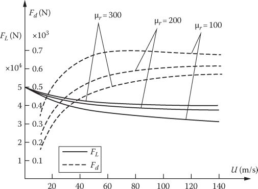
FIGURE 19.8 Levitation, F_l, and drag, F_d, forces versus speed. (After Boldea, I. and Nasar, S.A., Linear Motion Electromagnetic Systems, John Wiley & Sons, New York, 1985.)

For the example in Figure 19.7, the variation of levitation (attraction) force and of drag force, for different equivalent iron permeability, is shown in Figure 19.8.

A notable but not catastrophic decay of levitation force of 25% at 100 m/s and drag force F_d = 17% of acceleration force at 1 m/s² (0.7 × 10³ N), for a mass corresponding to the levitation force 4 × 10⁴ N (4 × 10³ kg), are observed.

The ratio (F_i/F_d)†_100m/s ≈ 4 × 10⁴/0.7 × 10³ = 57.1, which may be called the goodness factor of levitation, is considered good for high-speed MAGLEVs.

19.4 Preliminary Design Methodology

Based on an analytical or FEM-derived model, the design of the ALS starts with the sizing of the dc controlled electromagnets, capable of producing the rated and maximum attraction levitation forces F_Lr and F_Lmax for a required F_n/electromagnet weight ratio and for minimum copper losses in the electromagnet for that attraction force (copper loss/normal force).

The two criteria are conflicting, and this is why one was considered a constraint:

F L ( N ) g g G 0 ( kg ) > K l e v; K l e v = 7 - 15 (19.22)

$\frac{F_{L} (N)}{g_{g} G_{0} (kg)} > K_{l e v}; K_{l e v} = 7 - 15 (19.22)$

The higher values of K_lev correspond to forced cooling (j_con > (6–8) A/mm²), while the smaller values correspond to natural cooling (j = 3–3.5 A/mm²).

Higher current density j_con means not only a smaller coil but also larger copper losses per developed levitation force:

min (P c o F L) is desired (19.23)

$\min (\frac{P_{c o}}{F_{L}}) is desired (19.23)$

In addition, the guideway solid iron secondary (for levitation) has to be limited in weight (cost), and thus the total C-core electromagnet (and secondary) width is 2b_i +h_c < 0.3–0.35 m (there are two such secondary cores, one on each side of MAGLEVs). In a simplified form, this leaves room, for a given rated airgap Z_g to investigate the electromagnet length L versus width b_i (C-core leg width).

Images

FIGURE 19.9 Electromagnet mass to length L, levitation force/unit length, for j_con=3 A/mm² and j_con = 15 A/mm², versus C-core leg width d_i (a); recalculated mass with longitudinal end effect at 100 m/s (b). (After Matsumura, F. and Yamada, S., Elec. Eng. Jap., 94(6), 50, 1974.)

Let us continue the numerical example of Figures 19.7 and 19.8 and obtain, by using the simplified model in the previous paragraph, the results in Figure 19.9.

A visible increase in electromagnet weight is required to maintain the levitation force F_n=5 × 10⁴ N, to counteract the longitudinal end effect at v = 100 m/s.

When the C-core leg width is reduced, the cost of the track is reduced and also the electromagnet length L is increased; so the end effect influence is reduced. Values of L around 1.5 m are typical for high-speed MAGLEVs.

19.5 Dynamic Modeling of ALS Control

The single electromagnet guideway subsystem is presented in Figure 19.10.

It has only one degree of motion freedom along z (vertical) direction.

A MAGLEV involves multiple motions. But using secondary and tertiary mechanical suspension systems between the electromagnets and the bogie and between the latter and the passenger cabin, enough decoupling is obtained to allow for separate (decentralized) robust control of each electromagnet.

Images

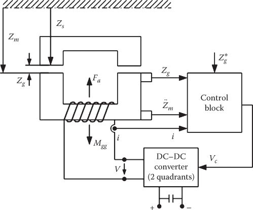
FIGURE 19.10 Single electromagnet-guideway system.

For stable levitation, the airgap Z_g is maintained close to the reference value Z_g*, within 20%–25% dynamically, in the presence of quite a few perturbations like external forces F_ext (from additional weight or wind forces) and guideway irregularities (from Z_s), such that a reasonable degree of ride comfort is secured for reasonable specific energy consumption (average kW/ton and peak kVA/ton).

To choose the input vector of variables, let us introduce here again the complete set of single electromagnet-guideway system equations:

V (t) = R i (t) + ψ ˙ (t) Ψ (t) = L (Z g, i) * i (t)

$\begin{array}{l} V (t) = R i (t) + \dot{ψ} (t) \\ Ψ (t) = L (Z_{g}, i) * i (t) \end{array}$

W m (t) = \int 0 Ψ i d Ψ; W c o m = i Ψ - W m (t) (19.24)

$W_{m} (t) = \int_{0}^{Ψ} i d Ψ; W_{c o m} = i Ψ - W_{m} (t) (19.24)$

F L = - \partial W m \partial Z g ∣ ∣ ∣ Ψ = c t = \partial W c o m \partial Z g ∣ ∣ ∣ i = c t

$F_{L} = - {\frac{\partial W_{m}}{\partial Z_{g}} |}_{Ψ = c t} = {\frac{\partial W_{c o m}}{\partial Z_{g}} |}_{i = c t}$

M Z ¨ m = M g - F L + F e x t; Z m = Z s + Z g (19.25)

$M {\ddot{Z}}_{m} = M_{g} - F_{L} + F_{e x t}; Z_{m} = Z_{s} + Z_{g} (19.25)$

It should be noticed that the motion equation now refers to the absolute acceleration Z_m and not to Z_g, because the guideway irregularities (visible in Z_s) are accounted for.

Using the approximations in (19.8) and (19.9),

Ψ = Ψ Z g + L l i; Ψ Z g = c i - d i 2 a z g + b (19.26)

$Ψ = Ψ_{Z_{g}} + L_{l} i; Ψ_{Z_{g}} = \frac{c i - d i^{2}}{a z_{g} + b} (19.26)$

F e \approx K x \cdot Ψ 2 Z g (19.27)

$F_{e} \approx K_{x} \cdot Ψ_{Z_{g}}^{2} (19.27)$

L_l is the leakage inductance of the electromagnet, considered independent of current i and position Z_g.

As visible in Equations 19.24 through 19.27, the single electromagnet guideway subsystem is nonlinear.

Linearization is used to pave the way for practical control system design.

For linearization,

V = V 0 + Δ V; ψ = ψ 0 + Δ ψ; i = i 0 + Δ i; F L = F L 0 + Δ F L; F e x t = F e x t 0 + Δ F e x t Z q = Z g 0 + Δ Z g; Z m = Z m 0 + Δ Z m; Z s = Z s 0 + Δ Z s (19.28)

$\begin{array}{l} \begin{matrix} V = V_{0} + Δ V; & ψ = ψ_{0} + Δ ψ; i = i_{0} + Δ i; F_{L} = F_{L_{0}} + Δ F_{L}; F_{e x t} = F_{e x t_{0}} + Δ F_{e x t} \end{matrix} \\ \begin{matrix} Z_{q} = Z_{g_{0}} + Δ Z_{g}; & Z_{m} = Z_{m_{0}} + Δ Z_{m} \end{matrix}; Z_{s} = Z_{s_{0}} + Δ Z_{s} \end{array} (19.28)$

Finally,

Δ V = R Δ i + α i Δ i ˙ + α g Δ Z ˙ g; α i = \partial Ψ \partial i ∣ ∣ 0; \partial Ψ \partial Z g ∣ ∣ 0 Δ F L = β i Δ Z g; β i = \partial F L \partial i ∣ ∣ 0; β g \partial F L \partial i ∣ ∣ 0 M Δ Z ¨ m = - Δ F L + Δ F e x t Δ Z m = Δ Z s + Δ Z g (19.29)

$\begin{array}{l} Δ V = R Δ i + α_{i} Δ \dot{i} + α_{g} Δ {\dot{Z}}_{g}; α_{i} = {\frac{\partial Ψ}{\partial i} |}_{0}; {\frac{\partial Ψ}{\partial Z_{g}} |}_{0} \\ Δ F_{L} = β_{i} Δ Z_{g}; β_{i} = {\frac{\partial F_{L}}{\partial i} |}_{0}; β_{g} {\frac{\partial F_{L}}{\partial i} |}_{0} \\ \begin{array}{l} M Δ {\ddot{Z}}_{m} = - Δ F_{L} + Δ F_{e x t} \\ Δ Z_{m} = Δ Z_{s} + Δ Z_{g} \end{array} \end{array} (19.29)$

⪻ Z_s (t )—for guideway irregularities—is considered given.

The coefficients α_i, α_g, β_i, β_g are calculated at the steady-state point characterized by V0,i0,Ψ0,FL0,Fext0,Zg0,Zm0 $V_{0}, i_{0}, Ψ_{0}, F_{L_{0}}, F_{e x t_{0}}, Z_{g_{0}}, Z_{m_{0}}$ and they are supposed to vary notably with the linearization “point.”

The structural diagram of the linearized model (19.28) and (19.29) is portrayed in Figure 19.11a, with Δ_i as the electrical variable.

A similar linearization is possible with ΔΨ instead of Δ_i as the electrical variable (Figure 19.11b) with

α ψ = \partial i \partial Ψ ∣ ∣ ∣ 0; β Ψ = \partial F L \partial Ψ ∣ ∣ ∣ 0; α g x = \partial i \partial Z g ∣ ∣ ∣ 0; β g x = \partial F L \partial Z g ∣ ∣ ∣ 0 (19.30)

$α_{ψ} = {\frac{\partial i}{\partial Ψ} |}_{0}; β_{Ψ} = {\frac{\partial F_{L}}{\partial Ψ} |}_{0}; α_{g x} = {\frac{\partial i}{\partial Z_{g}} |}_{0}; β_{g x} = {\frac{\partial F_{L}}{\partial Z_{g}} |}_{0} (19.30)$

Images

FIGURE 19.11 Linearized system with (a) Δ_i and (b) ΔΨ as the electrical variable.

Again, the coefficients α_Ψ, β_Ψ, α_gΨ, β_gΨ depend on the linearization point. It has been demonstrated that, being related to magnetic flux, which determines the levitation force irrespective of airgap Z_g0, they should vary less with Z_g0 in comparison with the coefficients for Δ_i as electric variable [11].

The problem is that, in general, the current may be measured (and controlled) easier than the flux linkage Ψ, especially at steady state (dc).

As the dynamic errors, introduced by linearization, depend heavily on the linearization point (Z_g0, F_L0, i₀...), especially with Δ_i as variable, when the linear control system is adopted, the latter is to be adaptive for MAGLEVs, where the airgap varies, at least at vehicle lift off and landing, by its rated value.

The structural diagrams suggest three possible state vectors:

Δ X 1 ¯ ¯ ¯ ¯ = ∣ ∣ ∣ ∣ ∣ Δ Z g Δ Z ˙ g Δ i ∣ ∣ ∣ ∣ ∣; Δ X 2 ¯ ¯ ¯ ¯ = ∣ ∣ ∣ ∣ ∣ Δ Z g Δ Z ˙ g Δ Z ¨ m ∣ ∣ ∣ ∣ ∣; Δ X 3 ¯ ¯ ¯ ¯ = ∣ ∣ ∣ ∣ ∣ Δ Z g Δ Z ˙ g Δ Ψ ∣ ∣ ∣ ∣ ∣ (19.31)

$Δ \underline{X_{1}} = | \begin{matrix} Δ Z_{g} \\ Δ {\dot{Z}}_{g} \\ Δ i \end{matrix} |; Δ \underline{X_{2}} = | \begin{matrix} Δ Z_{g} \\ Δ {\dot{Z}}_{g} \\ Δ {\ddot{Z}}_{m} \end{matrix} |; Δ \underline{X_{3}} = | \begin{matrix} Δ Z_{g} \\ Δ {\dot{Z}}_{g} \\ Δ Ψ \end{matrix} | (19.31)$

The output vectors for the three situations are

Δ Z g Δ i ∣ ∣ ∣ = ∣ ∣ ∣ 100001 ∣ ∣ ∣ Δ X 1, 2, 3 ¯ ¯ ¯ ¯ ¯ ¯ ¯ ¯ Δ Z g Δ Z ˙ g ∣ ∣ ∣ = ∣ ∣ ∣ 100001 ∣ ∣ ∣ Δ X 2, 1, 3 ¯ ¯ ¯ ¯ ¯ ¯ ¯ ¯ Δ Z g Δ Ψ ∣ ∣ ∣ = ∣ ∣ ∣ 100001 ∣ ∣ ∣ Δ X 3, 2, 1 ¯ ¯ ¯ ¯ ¯ ¯ ¯ ¯ (19.32)

$\begin{array}{l} \begin{matrix} Δ Z_{g} \\ Δ_{i} \end{matrix} | = | \begin{array}{l} 1 & 0 & 0 \\ 0 & 0 & 1 \end{array} | Δ \underline{X_{1, 2, 3}} \\ \begin{matrix} Δ Z_{g} \\ Δ {\dot{Z}}_{g} \end{matrix} | = | \begin{array}{l} 1 & 0 & 0 \\ 0 & 0 & 1 \end{array} | Δ \underline{X_{2, 1, 3}} \\ \begin{matrix} Δ Z_{g} \\ Δ_{Ψ} \end{matrix} | = | \begin{array}{l} 1 & 0 & 0 \\ 0 & 0 & 1 \end{array} | Δ \underline{X_{3, 2, 1}} \end{array} (19.32)$

From the structural diagrams in Figures 19.11a and b, we get state equations:

Δ X ˙ 1 = A 1 Δ X 1 + B 1 Δ V + C 1 ∣ ∣ ∣ Δ F e x t Δ Z ¨ s ∣ ∣ ∣ Δ X ˙ 2 = A 2 Δ X 2 + B 2 Δ V + C 2 ∣ ∣ ∣ ∣ ∣ Δ F e x t Δ F ˙ e x t Δ Z ¨ s ∣ ∣ ∣ ∣ ∣

$\begin{array}{l} Δ {\dot{X}}_{1} = A_{1} Δ X_{1} + B_{1} Δ V + C_{1} | \begin{matrix} Δ F_{e x t} \\ Δ {\ddot{Z}}_{s} \end{matrix} | \\ Δ {\dot{X}}_{2} = A_{2} Δ X_{2} + B_{2} Δ V + C_{2} | \begin{matrix} Δ F_{e x t} \\ Δ {\dot{F}}_{e x t} \\ Δ {\ddot{Z}}_{s} \end{matrix} | \end{array}$

Δ X ˙ 3 = A 3 Δ X 3 + B 3 Δ V + C 3 ∣ ∣ ∣ Δ F e x t Δ Z ¨ s ∣ ∣ ∣ (19.33)

$Δ {\dot{X}}_{3} = A_{3} Δ X_{3} + B_{3} Δ V + C_{3} | \begin{matrix} Δ F_{e x t} \\ Δ {\ddot{Z}}_{s} \end{matrix} | (19.33)$

The state variables have to be measured or some of them are to be estimated. In our case, Z_g may be measured by dedicated sensors; Z¨m ${\ddot{Z}}_{m}$ may be measured in general by an inertial sensor (ADx105 of analog devices).

The flux is not easily measurable, especially at steady state (dc), but Hall sensors with low temperature sensitivity could solve the problem.

However, Ż_g (even Z¨g ${\ddot{Z}}_{g}$ ) have to be estimated through an observer. Also, the flux Ψ may be observed if the Ψ(i, Z_g) FEM curve family is available (tabled or curve-fitted) and i and Z_g are measured directly. This way, even the flux at given current is observed.

Now if we calculate the transfer function between the airgap deviation ΔZ_g(s) and the input voltage ΔV(s), for zero external force and guideway irregularity perturbations (ΔF_ext (s) = 0, ΔZ_s(s) = 0) is of the form

Δ Z g Δ V ( s ) = - Δ V ( R + s α i ) ( ( s 2 M / β i ) + β g ) + α g s (19.33a)

$\frac{Δ Z_{g}}{Δ V (s)} = \frac{- Δ V}{(R + s α_{i}) ((s^{2} M / β_{i}) + β_{g}) + α_{g} s} (19.33a)$

It may be demonstrated that some roots of the denominator of Equation 19.33 have positive real parts at any linearization point (by the signs of α_i, β_i, α_g, β_g), and thus the open-loop voltage-fed system is not stable; even for controlled constant current, the system would be unstable.

The decrease in the levitation force with airgap increase is a strong phenomenological explanation for this.

As the system is statically and dynamically unstable, its forced stabilization is required.

19.6 State Feedback Control of ALS

Let us control the ALS linearized model with ΔX¯¯¯2=[ΔZg,ΔZ˙g,ΔZ¨m]T $Δ {\underline{X}}_{2} = {[Δ Z_{g}, Δ {\dot{Z}}_{g}, Δ {\ddot{Z}}_{m}]}^{T}$ as the state vector with the perturbation vector ΔZ¯¯¯2=[ΔFext,ΔF˙ext,ΔZ¨s]T $Δ {\underline{Z}}_{2} = {[Δ F_{e x t}, Δ {\dot{F}}_{e x t}, Δ {\ddot{Z}}_{s}]}^{T}$ and the output ΔY2¯¯¯¯=[ΔZg,ΔZ¨m]T $Δ \underline{Y_{2}} = {[Δ Z_{g}, Δ {\ddot{Z}}_{m}]}^{T}$ :

Δ X ˙ ¯ ¯ ¯ 2 = A Δ X ¯ ¯ ¯ 2 + B ¯ ¯ ¯ Δ Y ¯ ¯ ¯ 2 + P ¯ ¯ ¯ 2 Δ Z ¯ ¯ ¯ 2 (19.34)

$Δ {\underline{\dot{X}}}_{2} = A Δ {\underline{X}}_{2} + \underline{B} Δ {\underline{Y}}_{2} + {\underline{P}}_{2} Δ {\underline{Z}}_{2} (19.34)$

From (19.28 and 19.29),

A ¯ ¯ ¯ = ∣ ∣ ∣ ∣ ∣ 00 - β g / M 10 - (β g - β i α g / α i) / M 01 - R / α i ∣ ∣ ∣ ∣ ∣; B = ∣ ∣ ∣ ∣ ∣ 00 - β g / M α i ∣ ∣ ∣ ∣ ∣; P 2 ¯ ¯ ¯ ¯ = ⎡ ⎣ ⎢ 00 R / M α i 00 1 / M 0 - 1 0 ⎤ ⎦ ⎥ (19.35)

$\underline{A} = | \begin{matrix} 0 & 1 & 0 \\ 0 & 0 & 1 \\ - β_{g} / M & - (β_{g} - β_{i} α_{g} / α_{i}) / M & - R / α_{i} \end{matrix} |; B = | \begin{matrix} 0 \\ 0 \\ - β_{g} / M α_{i} \end{matrix} |; \underline{P_{2}} = [\begin{matrix} 0 & 0 & 0 \\ 0 & 0 & - 1 \\ R / M α_{i} & 1 / M & 0 \end{matrix}] (19.35)$

Though the control system should be adaptive, we hereby deal with it for one linearization point, only. The procedure may be repeated for a few critical situations and then the control law may use adaptable coefficients:

Δ V = K g Δ Z g + K u Δ Z ˙ g + K a Δ Z ¨ m = K T ¯ ¯ ¯ ¯ ¯ Δ X 2 ¯ ¯ ¯ ¯ (19.36)

$Δ V = K_{g} Δ Z_{g} + K_{u} Δ {\dot{Z}}_{g} + K_{a} Δ {\ddot{Z}}_{m} = \underline{K^{T}} Δ \underline{X_{2}} (19.36)$

such that integral squared criterion is minimum:

I (Δ V) = 1 2 \int 0 \infty [q 2 g Δ Z 2 g (t) + q 2 a Δ Z ¨ m (t) + Δ u 2 (t)] d t (19.37)

$I (Δ V) = \frac{1}{2} \int_{0}^{\infty} [q_{g}^{2} Δ Z_{g}^{2} (t) + q_{a}^{2} Δ {\ddot{Z}}_{m} (t) + Δ u^{2} (t)] d t (19.37)$

The control coefficients K_g, K_u K_a will depend on q_g and q_a in (19.37).

The optimum criterion (19.37) aim to

Reduce the airgap deviations (ΔZ_g) to avoid electromagnet-guideway collisions
Reduce absolute acceleration (Z¨m) $({\ddot{Z}}_{m})$ for ride comfort
Reduce control power (by ΔV)

The control law is obtained from the known equation:

K ¯ ¯ ¯ T = [K g K u K a] T = - R ¯ ¯ ¯ - 1 B T 2 P ¯ ¯ ¯ = - b' [P 13 P 23 P 33] T (19.38)

${\underline{K}}^{T} = {[\begin{matrix} K_{g} & K_{u} & K_{a} \end{matrix}]}^{T} = - {\underline{R}}^{- 1} B_{2}^{T} \underline{P} = - b^{'} {[\begin{matrix} P_{13} & P_{23} & P_{33} \end{matrix}]}^{T} (19.38)$

R ¯ ¯ ¯ = [1], b' = - β M α i, P ⇁ = ⎡ ⎣ ⎢ p 11 p 12 p 13 p 12 p 22 p 23 p 13 p 23 p 33 ⎤ ⎦ ⎥ (19.39)

$\begin{matrix} \underline{R} = [1], & b^{'} = \frac{- β}{M α_{i}}, & \underset{⇁}{P} = [\begin{matrix} p_{11} & p_{12} & p_{13} \\ p_{12} & p_{22} & p_{23} \\ p_{13} & p_{23} & p_{33} \end{matrix}] \end{matrix} (19.39)$

Matrix P is the solution of the Riccati equation:

P ¯ ¯ ¯ A ¯ ¯ ¯ 2 + A ¯ ¯ ¯ T 2 P ¯ ¯ ¯ - P ¯ ¯ ¯ \cdot B ¯ ¯ ¯ \cdot B ¯ ¯ ¯ T P ¯ ¯ ¯ = - Q ¯ ¯ ¯, Q ¯ ¯ ¯ = diag [q 2 g, 0, q 2 a] (19.40)

$\underline{P} {\underline{A}}_{2} + {\underline{A}}_{2}^{T} \underline{P} - \underline{P} \cdot \underline{B} \cdot {\underline{B}}^{T} \underline{P} = - \underline{Q}, \underline{Q} = diag [q_{g}^{2}, 0, q_{a}^{2}] (19.40)$

With known Q¯¯¯ $\underline{Q}$ , K^T (control law) may be calculated.

To determine Q¯¯¯ $\underline{Q}$ , Equation 19.40 is decomposed into six equations to find p₁₁, p₁₂, p₁₃, p₂₂, p₂₃, p₃₃. Then, using (19.38) and (19.39) and eliminating p₁₂, three equations with three unknowns are obtained:

K 2 g + 2 a 1 b K g = q 2 g (19.41)

$K_{g}^{2} + \frac{2 a_{1}}{b} K_{g} = q_{g}^{2} (19.41)$

K 2 a + 2 a 3 b ' K a + 2 b ' K u = q 2 a - 2 a 3 b ' K g - 2 a 1 b ' K a - 2 K g K a + 2 a 2 b ' K u + K 2 u = 0

$\begin{matrix} K_{a}^{2} + \frac{2 a_{3}}{b^{'}} K_{a} + \frac{2}{b^{'}} K_{u} = q_{a}^{2} \\ - \frac{2 a_{3}}{b^{'}} K_{g} - \frac{2 a_{1}}{b^{'}} K_{a} - 2 K_{g} K_{a} + \frac{2 a_{2}}{b^{'}} K_{u} + K_{u}^{2} = 0 \end{matrix}$

with

a 1 = - β g R M α i; a 2 = - β g M T d R α i; a 3 = - R α 1; T d = R α i + β i α g β g R

$\begin{matrix} a_{1} = \frac{- β_{g} R}{M α_{i}}; & a_{2} = \frac{- β_{g}}{M} \frac{T_{d} R}{α_{i}}; & a_{3} = - \frac{R}{α_{1}}; & T_{d} = \frac{R}{α_{i}} + \frac{β_{i} α_{g}}{β_{g} R} \end{matrix}$

Through an algebraic stability criterion,

K g > 2 K g 0 (k a - k a 0) (k u - k u 0) + (K g - K g 0 b ') \geq 0 (19.42)

$K_{g} > 2 K_{g 0} (k_{a} - k_{a 0}) (k_{u} - k_{u 0}) + (\frac{K_{g} - K_{g 0}}{b^{'}}) \geq 0 (19.42)$

where

K g 0 = β g R M α i b '; K u 0 = - β g R T d α i M b '; K a 0 = - R b ' α i (19.43)

$K_{g 0} = \frac{β_{g} R}{M α_{i} b^{'}}; K_{u 0} = \frac{- β_{g} R T_{d}}{α_{i} M b^{'}}; K_{a 0} = - \frac{R}{b^{'} α_{i}} (19.43)$

Also, the amplifiers have limits: Kg ≤ K_gmax; K_u < K_umax; and K_a < K_umax.

The system (19.41) has to have real solutions: K_g, K_a, K_u and thus q_g and q_a have to be chosen carefully in a domain. As the vehicle weight varies from unloaded mass (M₁) to loaded mass M₂, the q_a, q_g domain has to yield practical solutions for both situations.

For control implementations, we should notice that Z_g and Z_m are measurable, but Ż_g is not.

So an observer for Ż_g is required.

The control scheme with a state observer is illustrated in Figure 19.12 [11].

The Z_g observer in Figure 19.12 solves the problem of system behavior with respect to guideway irregularities.

It implies only the choice of S_ob = −β₀ pole since

Z ˙ ˆ g (1) = Z ¨ m ( 1 ) s + β 0 + s β 0 s + β 0 Z ˙ g (s) (19.44)

${\hat{\dot{Z}}}_{g} (1) = \frac{{\ddot{Z}}_{m} (1)}{s + β_{0}} + \frac{s β_{0}}{s + β_{0}} {\dot{Z}}_{g} (s) (19.44)$

For an ALS with the data M=200 kg, Z_g0 = 10⁻² m, T = α_i/R = 0.053 s, R = 1.532 Ω, β_i = 236 N A⁻¹, −β_g = 9 × 10⁵ N m⁻¹, results as in Figure 19.13 are obtained.

It is evident that without the adopted Z_g observer the system cannot tolerate force and track irregularity perturbations.

To further improve the performance, an integral of airgap error may be added to the control law to secure zero steady-state airgap error. Also an additional interior current loop may be added to limit the current and quicken the response.

A two-quadrant dc-dc converter (±V_max) is needed for quick enough control of MAGLEVs.

Images

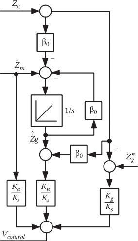
FIGURE 19.12 Control system with Zg observer (K_s: dc–dc converter gain).

Images

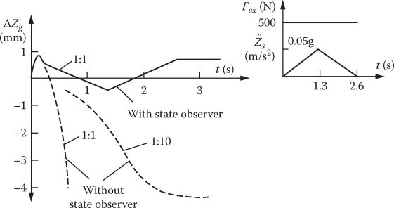
FIGURE 19.13 Control system response to external force F_ext and Z¨m ${\ddot{Z}}_{m}$ (track irregularities) perturbations. (After Matsumura, F. and Yamada, S., Elec. Eng. Jap., 94(6), 50, 1974.)

19.7 Control System Performance Assessment

The control system performance for MAGLEVs is related to

Electromagnet-guideway collision avoidance
Average control power
Ride comfort

For active magnetic bearings, in some applications, the maximum (or average) dynamic deviation of the airgap is limited to a small fraction of the rated airgap (when applied for machining purposes); ride comfort is not considered for active magnetic bearings but noise and vibration are.

To assess this performance, the following transfer functions of the close-loop system are required:

G 1 (s) = Z g ( s ) Z s ( s ) = - [ s 3 + ( R α i + β i K s K a M α i s 2 + K s β i M α i ) ] D ( s ) (19.45)

$G_{1} (s) = \frac{Z_{g} (s)}{Z_{s} (s)} = \frac{- [s^{3} + (\frac{R}{α_{i}} + \frac{β_{i} K_{s} K_{a}}{M α_{i}} s^{2} + \frac{K_{s} β_{i}}{M α_{i}})]}{D (s)} (19.45)$

G 2 (s) = Z g ( s ) F e x t ( s ) = 1 M ( s + R / K i ) D ( s ) (19.46)

$G_{2} (s) = \frac{Z_{g} (s)}{F_{e x t} (s)} = \frac{\frac{1}{M} (s + R / K_{i})}{D (s)} (19.46)$

G 3 (s) = Z g ( s ) V ( s ) = - β i M K i D ( s ) (19.47)

$G_{3} (s) = \frac{Z_{g} (s)}{V (s)} = \frac{- β_{i}}{M K_{i} D (s)} (19.47)$

with

D (s) = s 3 + (R K i + β i K s K a M α i) s 2 + (β i K s K a M α i) s + β i K s K g M α i + β g R M α i (19.48)

$D (s) = s^{3} + (\frac{R}{K_{i}} + \frac{β_{i} K_{s} K_{a}}{M α_{i}}) s^{2} + (\frac{β_{i} K_{s} K_{a}}{M α_{i}}) s + \frac{β_{i} K_{s} K_{g}}{M α_{i}} + \frac{β_{g} R}{M α_{i}} (19.48)$

The guideway (track) irregularities may be described by the power spectral density (PSD):

ϕ z (ω) : Φ z (ω) = A g U ω 2; U : vehiclespeed; A g : guideway constant (19.49)

$\begin{matrix} ϕ_{z} (ω) : \\ \begin{matrix} Φ_{z} (ω) = \frac{A_{g} U}{ω^{2}}; & U : vehiclespeed; & A_{g} : guideway constant \end{matrix} \end{matrix} (19.49)$

The squared average value of airgap deviations Z¯¯¯g ${\bar{Z}}_{g}$ caused by the guideway irregularities may be expressed by using G(1) from (19.45):

Z g ¯ ¯ ¯ ¯ = ⎡ ⎣ ⎢ \int 0.2 * π ω 0 | G 1 (j ω) | 2 ϕ z (ω) d ω ⎤ ⎦ ⎥ 1 / 2 (19.50)

$\bar{Z_{g}} = {[\int_{0.2 * π}^{ω_{0}} {| G_{1} (j ω) |}^{2} ϕ_{z} (ω) d ω]}^{1 / 2} (19.50)$

ω₀ is the maximum frequency of irregularities.

Z¯¯¯g ${\bar{Z}}_{g}$ may be considered a design value and should be a portion (0.2–0.25) of Z_g0 (for a good compromise between energy consumption and collision avoidance).

The average control power for known guideway irregularities is essential for a competitive system, and, for assessment, it is required first to calculate the voltage and current squared average deviations □V¯¯¯¯¯ $\bar{□ V}$ and □i¯¯¯¯ $\bar{□ i}$ :

Δ V ¯ ¯ ¯ ¯ ¯ = ⎡ ⎣ ⎢ \int 0.2 * π ω 0 ∣ ∣ ∣ G 1 ( j ω ) G 3 ( j ω ) ∣ ∣ ∣ 2 Φ z (ω) d ω ⎤ ⎦ ⎥ 1 / 2 (19.51)

$\bar{Δ V} = {[\int_{0.2 * π}^{ω_{0}} {| \frac{G_{1} (j ω)}{G_{3} (j ω)} |}^{2} Φ_{z} (ω) d ω]}^{1 / 2} (19.51)$

Δ i ¯ ¯ ¯ ¯ = ⎡ ⎣ ⎢ \int 0.2 * π ω 0 ∣ ∣ ∣ G 1 ( j ω ) * G - 1 3 ( j ω ) + ( α i - L l ) β i * j ω R + j ω α i ∣ ∣ ∣ 2 Φ z (ω) d ω ⎤ ⎦ ⎥ 1 / 2 (19.52)

$\bar{Δ i} = {[\int_{0.2 * π}^{ω_{0}} {| \frac{G_{1} (j ω) * G_{3}^{- 1} (j ω) + (α_{i} - L_{l}) β_{i} * j ω}{R + j ω α_{i}} |}^{2} Φ_{z} (ω) d ω]}^{1 / 2} (19.52)$

Thus, the average control power P_con is

P c o n = (V 0 + Δ V ¯ ¯ ¯ ¯ ¯) (I 0 + Δ i ¯ ¯ ¯ ¯) (19.53)

$P_{c o n} = (V_{0} + \bar{Δ V}) (I_{0} + \bar{Δ i}) (19.53)$

Finally, the ride comfort may be calculated using the power spectral density concept applied for absolute accelerations, ϕZ¨m(jω) $ϕ_{{\ddot{Z}}_{m}} (j ω)$ :

Φ Z ¨ m (ω) = ω 4 | G 1 (j ω) + 1 | 2 Φ z (ω) (19.54)

$Φ_{{\ddot{Z}}_{m}} (ω) = ω^{4} {| G_{1} (j ω) + 1 |}^{2} Φ_{z} (ω) (19.54)$

The human comfort level when exposed to a spectrum of accelerations of various frequencies has been quantified based on dedicated studies.

The “Janeway curve” is by now an accepted standard.

To meet the ride comfort standard, the ΦZ¨m(ω) $Φ_{{\ddot{Z}}_{m}} (ω)$ curve has to be below “Janeway curve” at all frequencies of interest.

The higher the speed, the more difficult it is to meet the “Janeway criterion.”

Even if it would be possible to meet the “Janeway criterion” at high speeds (say at U_max = 100 m/s), the energy consumption in the ALS might render the solution unpractical.

Consequently, a secondary (and a tertiary) mechanical suspension system is used on MAGLEVs.

A typical passive system is shown in Figure 19.14.

The secondary suspension system equations are

M Z ¨ M - M g - K (Z M - Z S - Z g - l 0) - β (Z ˙ M - Z ˙ m) (19.55)

$M {\ddot{Z}}_{M} - M g - K (Z_{M} - Z_{S} - Z_{g} - l_{0}) - β ({\dot{Z}}_{M} - {\dot{Z}}_{m}) (19.55)$

where

l₀ is the distance between unsprung (ALS) mass m and sprung mass M

K and β are the spring rigidity and damping coefficients when they are unloaded:

M g = K (Z M 0 - Z g 0 - l 0) (19.56)

$M g = K (Z_{M_{0}} - Z_{g_{0}} - l_{0}) (19.56)$

where

Z_M0 is the rated height of mass M

Z_g0 is the rated height of mass m

Images

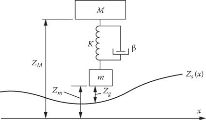
FIGURE 19.14 Passive secondary suspension system. (After Matsumura, F. and Yamada, S., Elec. Eng. Jpn., 94(6), 50, 1974.)

For the mass m, with no spring (the ALS),

m Z ¨ m = m g + K (Z M - Z S - Z g - l 0) + β (Z ˙ M - Z ˙ m) - F L + F e x t (19.57)

$m {\ddot{Z}}_{m} = m g + K (Z_{M} - Z_{S} - Z_{g} - l_{0}) + β ({\dot{Z}}_{M} - {\dot{Z}}_{m}) - F_{L} + F_{e x t} (19.57)$

In this case, the problem may be solved as up to now but with Zg¯¯¯¯ $\bar{Z_{g}}$ = (0.15–0.25)Z_g0; higher track irregularities may be tolerated or smaller average control power is obtained due to the presence of the secondary suspension system.

The ride comfort will be checked for Z_m ; in general, for a wise use of secondary system m/M < 0.2; a condition that is easily fulfilled by ALSs.

19.8 Control Performance Example

Let us suppose a MAGLEV of 50 ton at 100 m/s with rated airgap Z_g0=1.5 × 10⁻² m that uses electromagnets that are 1.5 m in length (L) with C = core leg width b_i = 0.04 m for a current density j_con = 15 A/mm² (forced cooling).

Ten electromagnets are used, so F_L0 = 5 × 10⁴ N with W_i0 = 3.58 × 10⁴ A-turns, V₀ = 200 V, I₀ = 200 A, electromagnet weight m=300 kg; coil resistance R = 1 Ω and the rated inductance L (saturation neglected) is L₀ = ∝_i=0.1 H, β_i = 1490 N/A, β_g = −1984 × 10⁷ N/m; L=Ψ/_i = (2.5 + 1.43/2 g)10⁻³(H).

Based on the control system design in Section 19.6, for q_a = 308 s²/m, q_g = 1.65 × 10⁵ V/m, we obtain the state feedback control law coefficients:

K g = 1.8 \times 105 V/m, K u = 1.07 \times 104 Vs/m, K a = 340.0 V s 2 /m

$K_{g} = 1.8 \times 10^{5} V/m, K_{u} = 1.07 \times 10^{4} Vs/m, K_{a} = 340.0 V s^{2} /m$

With these values, the transfer functions G₁ (s), G₂ (s), and G₃ (s) of (19.45) through (19.48) are

G 1 (s) \approx - ( s 3 + 964.0 s 2 + 3.18 \times 10 4 s ) D ( s ) G 2 (s) \approx 0.2 \times 10 - 3 s + 2.1 \times 10 - 3 D ( s ) G 3 (s) \approx - 2.98 D ( s ) D (s) \approx s 3 + 964 s 2 + 3.18 \times 104 s + 4.96 \times 105 (19.58)

$\begin{array}{l} G_{1} (s) \approx \frac{- (s^{3} + 964.0 s^{2} + 3.18 \times 10^{4} s)}{D (s)} \\ G_{2} (s) \approx \frac{0.2 \times 10^{- 3} s + 2.1 \times 10^{- 3}}{D (s)} \\ G_{3} (s) \approx - \frac{2.98}{D (s)} \\ D (s) \approx s^{3} + 964 s^{2} + 3.18 \times 10^{4} s + 4.96 \times 10^{5} \end{array} (19.58)$

With welded guideway, the constant A_g (in (19.49)) is A_g = 1.5 × 10⁻⁶ m.

From (19.50), the squared average airgap deviation Z_g = 4.6 × 10^-3 m < Z_g0/3 (f₀ = ω₀/2π = 25 Hz). Therefore, the MAGLEV avoids the collision with the guideway at 100 m/s. However, the squared average voltage and current deviations σ¯V ${\bar{σ}}_{V}$ and σ¯i ${\bar{σ}}_{i}$ are huge:

σ ¯ V = 4690 V; σ ¯ i = 670 A

${\bar{σ}}_{V} = 4690 V; {\bar{σ}}_{i} = 670 A$

The average control power is inadmissibly high, and thus a mechanical secondary system is needed.

To do so, we have to reconsider the whole control system design for m = 300 kg (only the electromagnet); finally, with q_a’ = 2.73 V s²/m, q_g’ = 5.8 × 10⁴ V/m, K_g’ = 7.4 × 10⁴, K_u’ = 5600, K_a’ = 14.8, Z¯¯¯′g ${\bar{Z}}^{'}_{g}$ = 4.65 × 10⁻³ m < Z_g0)/3, we obtain σ¯′ V ${\bar{σ}}^{'}_{V}$ =630.8 V, σ¯′i ${\bar{σ}}^{'}_{i}$ = 246.8 A.

This time the voltage deviation is about 3/1 and current deviation is 1.2/1. Such values are almost acceptable, but, if possible, they should be further reduced by the cabin’s additional suspension system contribution.

The ride comfort has been calculated (19.49) for both situations, and the results are shown in Figure 19.15.

Images

FIGURE 19.15 Ride comfort m = 300 kg, M = 5000 kg. (After Matsumura, F. and Yamada, S., Elec. Eng. Jpn.., 94(6), 50, 1974.)

The secondary system was not introduced in the data in Figure 19.15; only the mass M was decreased to m = 300 kg.

So a secondary (and tertiary) mechanical system is responsible to provide ride comfort for f > 5 Hz.

Vehicle lifting (from Z_gmax to Z_g0) and touchdown should be controlled by a special sequence, as the linear control system discussed so far may not be stable for such large airgap deviations.

This and other reasons raise the problem of alternative, more robust, control of ALS.

19.9 Vehicle Lifting at Standstill

For a 4 ton MAGLEV [9], similar to the previous, the state feedback control system was used for M = 1000 kg, Z_g0=0.01 m, R = 0.7 Ω, i₀=47 A, V₀=33 V, Ψ₀=∝i₀=5.20 Wb, K_g=5000.0, K_u = 3263, K_a = 110.0, ω_0s = 25 rad/s, and ξ = 0.45.

An additional flux linkage feedback is added to increase stability limits at large airgaps. A search coil voltage with a first-order large time constant delay is used for flux feedback Ψ_t (Figure 19.16).

Experimental results [9] (Figure 19.17) picturing the vehicle stable lifting (4 ALSs of 1 ton each) from 20 to 12.5 mm, with reasonable voltage and current dynamic profiles, tend to substantiate the benefic role of the flux feedback and of the airgap deviation PI loop, added to provide for ideally zero steady-state airgap deviation error.

The steady-state estimated average levitation control power is about 1.45 kW/ton, while the measured one was 1.54 kW/ton at standstill. As expected, naturally cooled electromagnets have been designed and thus their lift/weight ratio is only 7/1. For urban MAGLEVs (U ≤ 20 m/s), the average control power should in general be not more than two times the steady-state value (at standstill), which means about 3 kVA/ton. This is quite an acceptable value.

Images

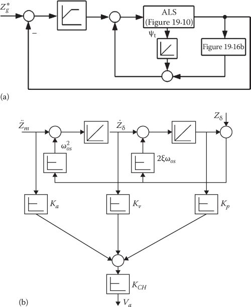
FIGURE 19.16 State feedback control system with additional flux feedback (a); observer (for Z˙ˆg ${\hat{\dot{Z}}}_{g}$ ) (b).

Images

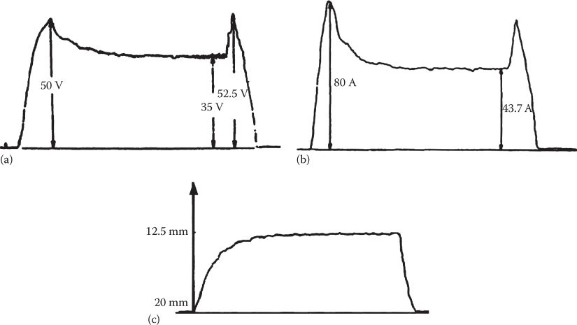
FIGURE 19.17 Experimental lifting of a 4 ton MAGLEV at standstill (4 × 1 ton ALSs): (a) input voltage (single quadrant dc-dc converter), (b) coil current, and (c) airgap (from 20 to 12.5 mm). (After Boldea, I. et al., IEEE Trans., VT-37(4), 213, 1988.)

19.10 Robust Control Systems for ALSs

It is by now evident that the state feedback control is sensitive to the linearization point and, when the airgap varies notably with respect to the linearization point, problems of stability in the presence of force and track irregularity perturbations occur.

To solve this problem, quite a few solutions have been recently proposed (mostly for active magnetic bearings).

Among such methods, we mention the following:

Gain scheduling derived from the linear parameter-dependent control initiated from the controllers defined at the corner of the parameter box [10]
Sliding mode control [11], which is known for its robustness to perturbations and parameter detuning; a sliding mode functional σ (Zg,Z˙g,Z¨g) $(Z_{g}, {\dot{Z}}_{g}, {\ddot{Z}}_{g})$ is first chosen:

$σ (Z g, Z ˙ m, Z ¨ m) = (Z * g - Z g) + T s Z ˙ ˆ g + T s T s m Z ˙ m (19.59)$ $σ (Z_{g}, {\dot{Z}}_{m}, {\ddot{Z}}_{m}) = (Z_{g}^{*} - Z_{g}) + T_{s} {\hat{\dot{Z}}}_{g} + T_{s} T_{s m} {\dot{Z}}_{m} (19.59)$

T_s is first to be imposed; in general T_s is smaller than the smallest time constant of the system. Then, T_sm has also to be chosen. The second-order functional σ (Zg,Z˙g,Z¨g) $(Z_{g}, {\dot{Z}}_{g}, {\ddot{Z}}_{g})$ = 0 represents a surface. If the system is capable of jumping to the σ (Zg,Z˙g,Z¨g) $(Z_{g}, {\dot{Z}}_{g}, {\ddot{Z}}_{g})$ = 0, then it will remain there under well-defined perturbation and parameter detuning limits.

The stability of SM control system is a problem in itself and may be treated in many ways but preferably (yet) by the Lyapunov method [11,12].

The control law is rather simple and may take the form [11]

V (t) = ⎧ ⎩ ⎨ ⎪ ⎪ ⎪ ⎪ ⎪ ⎪ ⎪ ⎪ ⎪ ⎪ ⎪ ⎪ + V max; K R σ (t) + 1 T i \int σ d t; - V max; σ (Z g, Z ˙ g) > h | σ | < h σ (Z ˙ g, Z ˙ g) < - h (19.60)

$V (t) = {\begin{array}{l} + V_{\max}; & σ (Z_{g}, {\dot{Z}}_{g}) > h \\ K_{R} σ (t) + \frac{1}{T_{i}} \int σ d t; & | σ | < h \\ - V_{\max}; & σ ({\dot{Z}}_{g}, {\dot{Z}}_{g}) < - h \end{array} (19.60)$

Here, ±V_max are the positive and negative maximum output voltages of the dc-dc converter that supplies the ALS.

Close to the target (|σ| < h), a PI controller over the SM functional is used to reduce chattering around the target. The parameters K_R and T_i have to be determined in the design process and have to be estimated as done for state feedback control systems.

But the PI system, which acts close to the target in corroboration with the term TsTsmZ¨m $T_{s} T_{s m} {\ddot{Z}}_{m}$ —via Z˙s ${\dot{Z}}_{s}$ , Equation 19.54, introduces a serious perturbation due to track irregularities [11].

To eliminate this perturbation, T_sm = 0 in (19.59), which becomes

σ s (Z g, Z ˙ g) = Z ¯ ¯ ¯ * g - Z g 0 + T s Z ˙ g (19.61)

$σ_{s} (Z_{g}, {\dot{Z}}_{g}) = {\bar{Z}}_{g}^{*} - Z_{g 0} + T_{s} {\dot{Z}}_{g} (19.61)$

But now, to reduce the perturbation influence, the SM control is cascaded with an interior fast (bipositional) current loop.

Typical results with such a system are shown in Figure 19.18 [11].

The airgap varies in Figure 19.18a from 0.03 to 0.01 m and, respectively, to 0.005 m. The response time is about 0.2 s. The perturbation rejection looks very good, and this is due to the fast current (bipositional) loop response; Z¨s ${\ddot{Z}}_{s}$ is followed strictly by Z¨m ${\ddot{Z}}_{m}$ toward its rejection.

The fast current and force responses (Figure 19.18b) are evident. The high-frequency oscillations in the current loop are visible in force also, but they are limited and may be handled by standard insulate gate bipolar transistor (IGBT) dc-dc converters.

Moreover, the current fast (PD) current loop reduces the system to one of second order.

Images

FIGURE 19.18 SM + current control: (a) airgap, Z˙gZ¨mZ¨s ${\dot{Z}}_{g} {\ddot{Z}}_{m} {\ddot{Z}}_{s}$ with details (zoom). SM+current control: (b) current, external force, σ(Z_g, Ż_g) with details (zoom). (After Trica, Al., Electromagnetic Suspension Systems, University Politehnica Timisoara Publishers, 2009.)

Images

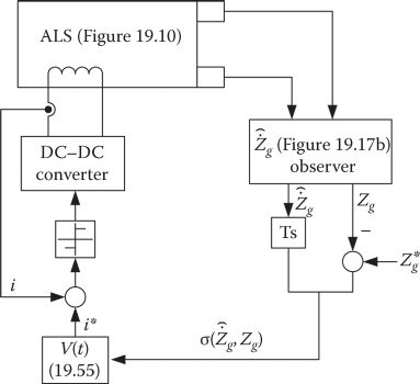
FIGURE 19.19 SM + PI + current control system.

Note: Though the absolute acceleration Z¨m ${\ddot{Z}}_{m}$ disappears from the sliding mode functional (19.61), it remains in the system model for the design of the sliding mode controllers.

Therefore, the SM + PI + current loop control system looks as in Figure 19.19 (For more on SM control, see Ref. [12]).

It appears that such a simple control system is very robust. It remains to be seen if the rather increased maximum voltage V_max is acceptable for the application.

State feedback control with current change rate feedback of dual-sided ASL system (for linearization of levitation force with current and airgap) applied to an active magnetic bearing was shown to produce sensorless airgap control [13].
The dual ALS for suspension together with one for guidance for MAGLEV transportation industrial platform is proportional integral derivative (PID)-fuzzy adaptive controlled differentially in a master-slave solution with I₀ ± i [14] (Figure 19.20a and b).

Images

FIGURE 19.20 MAGLEV industrial transport platform: (a) framework, (b) control system for levitation (vertical motion), (c) optimized geometry for levitation (vertical motion) and guidance (lateral motion). MAGLEV industrial transport platform: (d) six airgaps evolution during MAGLEV motion. (After Li, L. et al., IEEE Trans., MAG-40, 3512, 2004.)

Images

Airgap eddy current sensors with 0.1 μm resolution are used.

Another dual PM-assisted ALS (intended for axial active magnetic bearings Figure 19.2b) has been shown to produce a resultant attraction force F_L proportional to current and displacement from middle position, which makes it easier to control:

F L = K i I + K x X (19.61a)

$F_{L} = K_{i} I + K_{x} X (19.61a)$

over the entire airgap range [15].

19.11 Zero Power Sliding Mode Control for PM-Assisted ALSs

As shown in Figure 19.2a and b, PM-assisted ALS may also be considered (Figure 19.21).

The control of such a system is similar to that of dc controlled ALS presented so far, but here quite a different approach is taken for the description of the four operation modes to be handled, integrated by ALS:

Smooth takeoff with switching to zero power control afterward.
Zero control power levitation: The steady-state control coil current is maintained to zero even with payload variation, but the targeted airgap will now vary such that the PM alone may produce the whole levitation force.
Guideway collision avoidance control takes over and controls the system at minimal airgap.
Soft landing is provided by planned airgap versus time reference tracking control.

Images

FIGURE 19.21 PM-assisted ALS.

For zero power (current) control, sliding mode control is adopted for robustness, but first one new row is added in the state-space model, which contains ∫∆idt [16]:

∣ ∣ ∣ ∣ ∣ ∣ ∣ ∣ Δ Z g Δ Z ˙ g \int Δ i d t Δ i ∣ ∣ ∣ ∣ ∣ ∣ ∣ ∣ = ∣ ∣ ∣ ∣ ∣ ∣ 0 a 210 + Δ a 21 00 100 a 420 + Δ a 42 0000 0 a 240 + Δ a 24 1 a 440 + Δ a 44 ∣ ∣ ∣ ∣ ∣ ∣ ∣ ∣ ∣ ∣ ∣ ∣ ∣ ∣ Δ Z g Δ Z ˙ g \int Δ i d t Δ i ∣ ∣ ∣ ∣ ∣ ∣ ∣ ∣ + ∣ ∣ ∣ ∣ ∣ ∣ 000 b ∣ ∣ ∣ ∣ ∣ ∣ Δ V + ∣ ∣ ∣ ∣ ∣ ∣ 0 d 0 b ∣ ∣ ∣ ∣ ∣ ∣ F e x t + ∣ ∣ ∣ ∣ ∣ ∣ 0100 ∣ ∣ ∣ ∣ ∣ ∣ Z ¨ s | A | = | A 0 | + | Δ A | (19.62)

$\begin{matrix} | \begin{matrix} Δ Z_{g} \\ Δ {\dot{Z}}_{g} \\ \int Δ i d t \\ Δ i \end{matrix} | = | \begin{matrix} 0 & 1 & 0 & 0 \\ a_{210} + Δ a_{21} & 0 & 0 & a_{240} + Δ a_{24} \\ 0 & 0 & 0 & 1 \\ 0 & a_{420} + Δ a_{42} & 0 & a_{440} + Δ a_{44} \end{matrix} | | \begin{matrix} Δ Z_{g} \\ Δ {\dot{Z}}_{g} \\ \int Δ i d t \\ Δ i \end{matrix} | + | \begin{matrix} 0 \\ 0 \\ 0 \\ b \end{matrix} | Δ V + | \begin{matrix} 0 \\ d \\ 0 \\ b \end{matrix} | F_{e x t} + | \begin{matrix} 0 \\ 1 \\ 0 \\ 0 \end{matrix} | {\ddot{Z}}_{s} \\ | A | = | A_{0} | + | Δ A | \end{matrix} (19.62)$

and

a 210 = 1 M \partial F L \partial Z g ∣ ∣ 0, a 240 = 1 M \partial F L \partial i ∣ ∣ 0, a 420 = - w 1 \partial Φ \partial Z g ∣ ∣ 0, a 440 = - R L 0, b = 1 L 0, d = 1 M (19.63)

$\begin{matrix} a_{210} = \frac{1}{M} {\frac{\partial F_{L}}{\partial Z_{g}} |}_{0}, & a_{240} = \frac{1}{M} {\frac{\partial F_{L}}{\partial i} |}_{0}, & a_{420} = {\frac{- w_{1} \partial Φ}{\partial Z_{g}} |}_{0}, & a_{440} = \frac{- R}{L_{0}}, & b = \frac{1}{L_{0}}, & d = \frac{1}{M} \end{matrix} (19.63)$

where

L₀ is the coil inductance at rated airgap

M is the ALS mass

R is the coil resistance

Z_m is the track irregularities acceleration

The similarity with previous paragraphs (19.6) is strong; just a new row is added.

A sliding hyperplane σ, its reaching law σ, and the control law ΔV are defined as [16]

σ = C ¯ ¯ ¯ \cdot X ¯ ¯ ¯; C ¯ ¯ ¯ = [C 1 C 2 C 1 K, 1]; X ¯ ¯ ¯ = [Δ Z g, Δ Z ˙ g \int Δ i d t, Δ i] T (19.64)

$\begin{matrix} σ = \underline{C} \cdot \underline{X}; & \underline{C} = [C_{1} C_{2} C_{1} K, 1]; & \underline{X} = {[Δ Z_{g}, Δ {\dot{Z}}_{g} \int Δ i d t, Δ i]}^{T} \end{matrix} (19.64)$

with

σ ˙ = - p σ - q s i g n (σ) (19.65)

$\dot{σ} = - p σ - q s i g n (σ) (19.65)$

and

Δ V = (C ¯ ¯ ¯ b - 1) (- C ¯ ¯ ¯ A 0 X ¯ ¯ ¯ - p σ - q s i g n (σ)) (19.66)

$Δ V = (\underline{C} b^{- 1}) (- \underline{C} A_{0} \underline{X} - p σ - q s i g n (σ)) (19.66)$

If the system characteristic on the hyperplane is chosen as [16]

C F (s) = (s + t ω n) (s 2 + 2 ξ ω n s + ω 2 n) (19.67)

$C F (s) = (s + t ω_{n}) (s^{2} + 2 {ξω}_{n} s + ω_{n}^{2}) (19.67)$

then the parameters of the control law C₁, C₂, and K may be calculated as

C 1 = 2 ξ ω 2 n + ω 2 n + a 210 a 240 C 2 = ( t ω n + 2 ξ ω n + t ω 3 n ) / a 210 a 240 K = - t ω 3 n a 210 \cdot c 1 (19.68)

$\begin{array}{l} C_{1} = \frac{2 {ξω}_{n}^{2} + ω_{n}^{2} + a_{210}}{a_{240}} \\ C_{2} = \frac{(t ω_{n} + 2 {ξω}_{n} + t ω_{n}^{3}) / a_{210}}{a_{240}} \\ K = \frac{- t ω_{n}^{3}}{a_{210} \cdot c_{1}} \end{array} (19.68)$

For stability, not only p > 0 and q > 0 in (19.65) [17], but also the external force is estimated as

F ˆ e x t = M \cdot a 210 \cdot K \int Δ i d t (19.69)

${\hat{F}}_{e x t} = M \cdot a_{210} \cdot K \int Δ i d t (19.69)$

From the existence condition of the sliding hyperplane, σσσ < 0, the values of p and q are obtained as

p > sup ∣ ∣ ∣ C ¯ ¯ ¯ Δ A + Z ¨ s σ ∣ ∣ ∣ > 0 q = ∣ ∣ ∣ c 2 a 210 K \int Δ i d t ∣ ∣ ∣ > 0 (19.70)

$\begin{array}{l} p > \sup | \frac{\underline{C} Δ A + {\ddot{Z}}_{s}}{σ} | > 0 \\ q = | c_{2} a_{210} K \int Δ i d t | > 0 \end{array} (19.70)$

On a 25 kg empty vehicle in Ref. [16], a 12 kg payload is added and the airgap response is shown in Figure 19.22.

It is now evident that the steady-state current is driven to zero after the airgap is reduced from 9.00 to 6.5 mm (such that the PMs alone can handle the entire larger levitation force).

Images

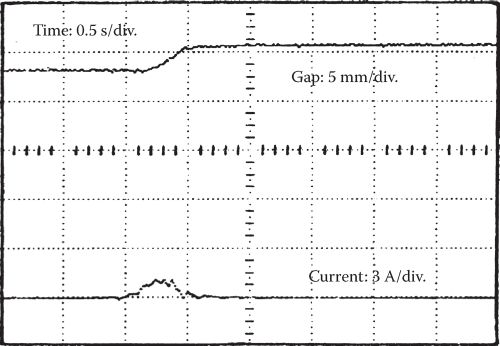
FIGURE 19.22 Airgap and current response for 12 kg payload addition (to 25 kg dead weight).

For vehicle takeoff and soft landing, as well as operation at minimum airgap safety rides, the airgap tracking mode should be initiated.

This time the state space model gets an additional state of ∫ΔZ′g $\int Δ {Z^{'}}_{g}$ dt (in fact, it gets the equality (∫ΔZ′gdt)′=ΔZ′g) ${(\int Δ {Z^{'}}_{g} d t)}^{'} = Δ {Z^{'}}_{g})$ ; and thus the current will be automatically adjusted to a nonzero value such as

Δ i - T \int Δ Z' g d t \to 0 (19.71)

$Δ i - T \int Δ {Z^{'}}_{g} d t \to 0 (19.71)$

The state space vector is similar to that mentioned previously, that is, X¯¯¯=[∫ΔZ′gdt,ΔZg,ΔZ˙g,Δi] $\underline{X} = [\int Δ {Z^{'}}_{g} d t, Δ Z_{g}, Δ {\dot{Z}}_{g}, Δ i]$ , and so are the sliding hyperplanes σ^/,(σ˙′ ${\dot{σ}}^{'}$ and ΔV’. The design of the controller is similar to the one for zero current control, and the two modes may be integrated into a single control system.

Reference [16] shows a typical planned soft takeoff and landing (Figure 19.23).

Also Figure 19.23c shows minimum (safe) airgap tracking control for maximum overload (additional 25 kg for 25 kg dead weight).

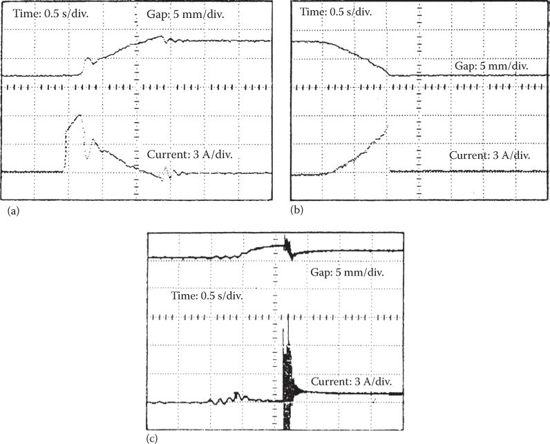
The control performance is evaluated as done previously in this chapter with respect to rms airgap variation, average control power, and ride comfort ((19.45) through (19.48)), only to find that Z¯¯¯g/Zg0 ${\bar{Z}}_{g} / Z_{g 0}$ = 1/7 and P_con = 0.32 kW/ton for a full-size 400 km/h MAGLEV [18]. Compared to at least 3 kW/ton for a dc-controlled electromagnet ALS, it seems some spectacular progress. But the cost of the PMs for high-speed MAGLEVs should not be underestimated; however, for MAGLEV industrial platforms, the zero power control via sliding modes seems to us quite practical.

Images

FIGURE 19.23 (a) Takeoff from 14 to 9 mm, (b) soft landing, and (c) overload (25 kg payload) operation at minimum airgap (5 mm). (After Tzeng, Y.K. and Wang, T.C., Analysis and experimental results of a MAGLEV transportation system using controlled—PM electromagnets with decentralized robust control strategy, Record of LDIA–1995, Nagasaki, Japan, pp. 109–113, 1995.)

19.12 Summary

ALS provide stable equilibrium of an electromagnet below a mild steel body, at a reference distance by active control of the current in the electromagnet; an ALS uses electromagnetic attraction force as expressed in Maxwell tensor.
ALS applications range from magnetic bearings through industrial platforms to vehicular MAGLEVs (at medium and high speed).
The primary electromagnet may be provided also with a PM when the current control in the electric coil serves mostly for airgap control.
For PM-assisted ALS, it is feasible to operate at variable airgaps when the payload increases such that only the PMs provide the steady-state levitation force when the steady-state current is zero; nonzero current occurs only during transients; this is called zero current (power) control.
In MAGLEV vehicle applications, the secondary of an ALS is made of solid iron for economic reasons. However, during control and vehicle motion at high speeds, eddy currents are induced in the solid iron secondary/track. These eddy currents reduce the levitation force F_L0 and produce a drag force F_d; both have to be calculated and considered in the design of ALS for medium-/high-speed MAGLEVs (20–100 m/s).
The design of ALS starts with the specifications of F_L/ALS weight, rated voltage, current, speed, and secondary width L_W interval and calculates essentially the electromagnets number, length L, and C-core leg width b_i.
Then, after a first geometry is obtained, longitudinal end effects on F_L and F_d are calculated at maximum speed; the design is corrected iteratively until the value of F_L is the desired one, with end longitudinal effects considered.
It has been shown that even at 100 m/s, the normal force is reduced only by about 25% and the drag force corresponds to 0.1 m/s deceleration of the vehicle due to longitudinal end effects. So ALSs are suitable for high-speed MAGLEVs.
The copper losses per levitation force (or vehicle weight) is another performance criterion to be checked; 3–4 kW/ton at 100 m/s is considered reasonable and ALSs are capable of that, but only if a secondary mechanical suspension system is added; for full comfort a tertiary (cabin) mechanical suspension system is used.
The state space equations of ALS are nonlinear; after linearization they prove to correspond to a statically and dynamically unstable system; so stabilization has to be forced on it by close-loop control.
State feedback control with Zg,Z˙ˆg,Z¨m $Z_{g}, {\hat{\dot{Z}}}_{g}, {\ddot{Z}}_{m}$ (absolute acceleration) as the state vector and Zg,Z¨m $Z_{g}, {\ddot{Z}}_{m}$ as output vector has been proven, after the linearization, to allow for smaller coefficients variation with linearization point conditions. So an airgap sensor and an absolute acceleration sensor are needed. The track irregularities are represented by Ż_s(t),
State feedback control may be designed using an optimization criterion that secures electromagnet-guideway collision avoidance, ride comfort, and limited control power.
As Ż_g cannot be measured, an observer is needed; particular observer properties are necessary to handle track irregularity perturbations.
Dedicated transfer functions (19.45 through 19.48) are used to calculate performance indices:
- rms airgap deviation error: Z¯¯¯g ${\bar{Z}}_{g}$
- Voltage and current rms deviations: □V¯¯¯¯¯,□i¯¯¯¯ $\bar{□ V}, \bar{□ i}$

Ride comfort: ϕZ¨m $ϕ_{{\ddot{Z}}_{m}}$ (ω)

By a numerical example it is proven that even without a mechanical suspension system ALS may provide Z¯¯¯g/Zg0 ${\bar{Z}}_{g} / Z_{g 0}$ < 0.33 (to avoid collisions with the track) but at huge voltage ΔV¯¯¯¯¯/V0 $\bar{Δ V} / V_{0}$ = 20 and large current rations Δi¯¯¯¯/i0 $\bar{Δ i} / i_{0}$ > 3 at 100 m/s. Consequently, secondary and tertiary mechanical suspension systems are needed to handle the control at reasonable control power and good ride comfort above 5 Hz, in 100 m/s (or so) MAGLEVs.
The vehicle lifting (take off) and landing requires special control as state feedback control cannot handle such large variations of airgap. More robust control to handle both running and lifting and landing of the vehicle is needed.
Sliding mode control, plus a PI control close to the target and an interior fast (bi-positional) current loop, has been proven capable of handling most operation modes of a mediumspeed (15–20 m/s) MAGLEV at less than 2.5 kW/ton control power and airgap variation from 20 mm (idle position) to the rated 10 mm.
Also state feedback control plus a flux feedback was shown to be proper for robust control of ALS.
Finally, sliding mode zero power (current) control for running and SM nonzero current control for takeoff and landing with airgap planned trajectory tracking have been proven to be adequate for PM-assisted ALSs. A calculated spectacular 0.36 kW/ton control power at 100 km/h suggests that PM-assisted ALSs should be given more consideration in the future, especially for an industrial platform.
At the other end of the scale, for axial/magnetic bearings, a PM-assisted ALS has been proven, even by PID + SM + current control, capable for large axial force perturbation rejection for speed transients of ±18 krpm [19].
Even the placement of a high-temperature superconductor to produce constant-width-airgap attraction force has been proven to be adequate for simplified control ALSs.
It is estimated that ALS will spread more in the future due to low energy consumption, low noise and vibration in transportation of people or in industry, and for industrial MAGLEV platforms [20].

References

1. H. Kemper, Suspension systems through electromagnetic forces, a possible approach to basically new transportation technologies, ETZ, 4, 1933, 391–395 (in German).

2. H. Kemper, Electrical railroad vehicles magnetically guided, ETZ-A, 1, 1953, 11–14 (in German).

3. G. Bohn, P. Romstedt, W. Rothmayer, and P. Schwarzler, A contribution to magnetic levitation technology, Proceedings of the Fourth ICEC, Eindhoven, the Netherlands, 1972, pp. 202–208.

4. R.M. Borcherts and L.C. Davis, Lift and drag forces for the attraction electromagnetic systems, Ford Motor Company Scientific Research Staff Report, 1976.

5. S. Yamamura and T. Ito, Analysis of speed characteristics of the attractive electromagnetic levitation vehicles, Elec. Eng. Jap., 95(162), 1975, 84–89.

6. I. Boldea and S.A. Nasar, Linear Motion Electromagnetic Systems, Chapter 10, John Wiley & Sons, New York, 1985.

7. I. Boldea, Optimal design of attraction levitation magnets including the end effect, EME (now EPCS) J., 6, 1981, 57–66.

8. F. Matsumura and S. Yamada, A method to control the suspension system utilizing magnetic attraction force, Elec. Eng. Jpn., 94(6), 1974, 50–57.

9. I. Boldea, A. Trica, G. Papusoiu, and S.A. Nasar, Field tests on MAGLEV with passive guideway linear inductor motor transportation system, IEEE Trans., VT-37(4), 1988, 213–219.

10. A. Forrai, T. Ueda, and T. Yumura, Electromagnetic actuator control: A linear parameter—Varying (LPV) approach, IEEE Trans., 1E-54(3), 2007, 1440–1441.

11. Al. Trica, Electromagnetic Suspension Systems, University Politehnica Timisoara Publishers, 2009 (in Romanian).

12. V. Utkin, J. Guldner, and J. Shi, Sliding Mode Control in Electromechanical Systems, 2nd edn., CRC Press, Taylor & Francis Group, New York, 2009.

13. L. Li, T. Shinshi, and A. Shimokohbe, State feedback control of active magnetic bearing based on current change rate alone, IEEE Trans., MAG-40, 2004, 3512–3517.

14. J.A. Duan, H.B. Zhou, and N.P. Guo, Electromagnetic design of a novel linear MAGLEV transportation platform with finite element analysis, IEEE Trans., MAG-47(1), 2011, 260–263.

15. D. Wu, X. Xie, and S. Zhou, Design of a normal stress electromagnetic fast linear actuator, IEEE Trans., MAG-46(4), 2010, 1007–1014.

16. Y.K. Tzeng and T.C. Wang, Analysis and experimental results of a MAGLEV transportation system using controlled—PM electromagnets with decentralized robust control strategy, Record of LDIA-1995, Nagasaki, Japan, 1995, pp. 109–113.

17. W. Gao and J.C. Hung, Variable structure control of linear system: A new approach, IEEE Trans., 1E-40(1), 1993, 45–55.

18. Y.K. Tzeng and T.C. Wang, Dynamic analysis of the MAGLEV system using controlled—PM electromagnets with robust zero power control strategy, Record of IEEE Intermag 1995, San Antonio, TX, 1995.

19. K. Hijikata, M. Takemoto, S. Ogasawara, A. Chiba, and T. Fukao, Behavior of a novel thrust magnetic bearing with a cylindrical rotor on high speed rotation, IEEE Trans., MAG-45(10), 2009, 4617–4620.

20. M. Ghodsi, T. Ueno, and T. Higuchi, Improvement of magnetic circuit in levitation system using HTS and soft magnetic material, IEEE Trans., MAG-41(10), 2005, 4003–4005.

..................Content has been hidden....................

You can't read the all page of ebook, please click here login for view all page.

Table of Contents for Chapter 19 Attraction Force (Electromagnetic) Levitation Systems

Create new playlist

Sign In

Sign Up

Table of Contents for
Chapter 19 Attraction Force (Electromagnetic) Levitation Systems