Chapter 16 Linear DC PM Brushless Motors

Search in book...
Toggle Font Controls
Create new playlist

Name your new playlist

Playlist description (optional)
Sign In

Email address

Password

Forgot Password?

or

Continue with Facebook

Continue with Google
Sign Up

Full Name

Email address

Confirm Email Address

Password

or

Continue with Facebook

Continue with Google

The linear dc homopolar-PM motor has been developed from the voice-coil speaker-microphone linear electromagnetic device; however, in most cases, it uses a flat (rather than tubular) topology and is applied for progressive (rather than oscillatory) linear motion; also, the travel may reach 100 mm or more.

As it is based on Lorenz force, to change direction of motion the polarity of the current is reversed [1–3]. The main asset is the simplicity of the control with full force starting from any position when supplied from a 4 quadrant dc–dc converter, for a rather long (100 mm or even more), but limited, travel. Short coil mover with long PM or long coil stator with short PM-mover combinations may be used, depending on the application.

The copper losses per N of thrust are not small as the coil is in the air, to avoid any cogging (zero current) force and thus allow for precision control.

Recording pens, optical disk drives, focusing systems in digital video cameras, x–y chart recorders, etc., are typical applications of linear dc PM brushless motors [4–9].

Linear dc PM brush motors have also been proposed [1], but today these are of mere historical interest; consequently, only brushless topologies are considered.

Finally, as tubular configurations will be investigated for linear oscillatory machines in a subsequent chapter, only flat configurations will be treated in this chapter.

Design issues of iron-core-backed or air-core-backed PM topologies are studied in some detail; then iron losses and geometrical optimization design are illustrated; finally, sliding mode precision control is investigated, as applied in focusing a digital video camera.

16.2 Topology Aspects

Two basic topologies are shown in Figure 16.1a and b [3,8].

The single-coil mover in Figure 16.1a—intended for travels above 10 mm—allows for a larger force density than the dual-coil mover with PM in air (Figure 16.1b), but the latter has a larger force/weight, so crucial in some applications, when the mover has a small weight (1–2 g). For larger force per volume, single-coil dual-core configurations may be used (Figure 16.2).

As the thin magnetic fixture may be replaced even with a nonmagnetic rugged one, the inductance of the coil is rather small and thus the force variation with mover position is very small, because the core magnetic saturation under load is not large, provided the PM flux does produce a reasonable flux density in the core. Also, the iron losses are to be smaller as they are produced mainly by the local variation of the core magnetic flux density due to armature current.

Out of the four coil sides, this time two are active (only one side is active in Figure 16.1); this justifies the claims of larger force density and lower copper losses per N of force. Lateral nonmagnetic plates (Figure 16.2b) may provide better PM stiffness over PM length up to 0.1–0.15 m travel or even more.

To double the thrust for the single coil, the PM thickness has to be doubled (roughly), but the core weight is only slightly larger (20% or so) while the coil weight is also only slightly increased (20% or so). The configuration in Figure 16.2 shows further potential for improvements in linear dc PM brushless topologies.

Images

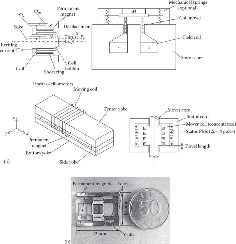
FIGURE 16.1 Basic topologies: (a) with one-coil mover and iron cores, (b) with PM in air and dual-coil mover.

16.3 Principle and Analytical Modeling

Let us consider here the analytical model of the configuration in Figure 16.1a, illustrated in more detail in Figure 16.3.

With N turns per coil, w_c, active coil length and B_PM, PM flux density, considered uniform here along x (direction of motion), the Lorenz force on the coil F_x is

F_{x} = K_{f} \cdot i; K_{f} = B_{P M} \cdot N \cdot w_{c} (16.1)

$F_{x} = K_{f} \cdot i; K_{f} = B_{P M} \cdot N \cdot w_{c} (16.1)$

Images

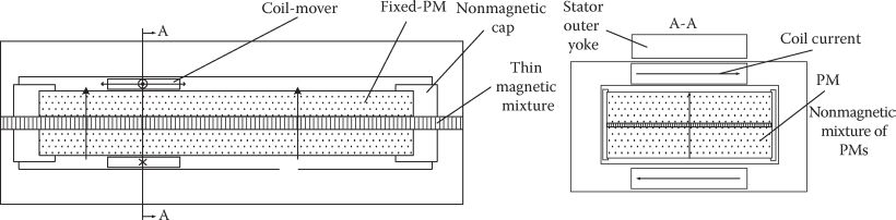
FIGURE 16.2 Single-coil dual-core configuration.

Images

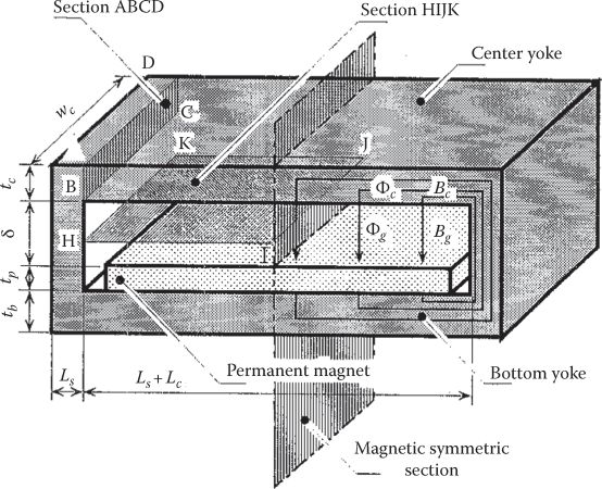
FIGURE 16.3 Geometry and flux paths of linear dc PM mover. (After Wakiwaka, H. et al., IEEE Trans., MAG-32(5), 5073, 1996.)

At center point, the PM flux and the armature (coil mmf) flux lines and flux density distribution are given in Figure 16.4.

As visible in Figure 16.4, the armature reaction increases the core flux on the right side of mover and decreases it on the left side, much like in a standard rotary dc brush motor (transversal armature reaction).

Now, with the mover at extreme position, the coil (armature) flux stays the same (within the core) while the PM fringing (leakage) at its ends leads to an even smaller force. So K_f is expected to vary with mover position due to magnetic saturation (Figure 16.4c) because the field of the coil mmf closes mainly within the magnetic core.

This reality would become evident with 3D FEM (even with 2D FEM) analysis, but an approximate analysis, valid for preliminary design, would be in order here.

So let us consider the center position when the flux produced in the core by the coil is

ϕ = B_{a} \cdot w_{c} \cdot t_{c}; B_{a} = \frac{N i μ (B_{c})}{2 (L_{s} + L_{c} + l_{s} + t_{p} + g + t_{c})} (16.2)

$ϕ = B_{a} \cdot w_{c} \cdot t_{c}; B_{a} = \frac{N i μ (B_{c})}{2 (L_{s} + L_{c} + l_{s} + t_{p} + g + t_{c})} (16.2)$

Images

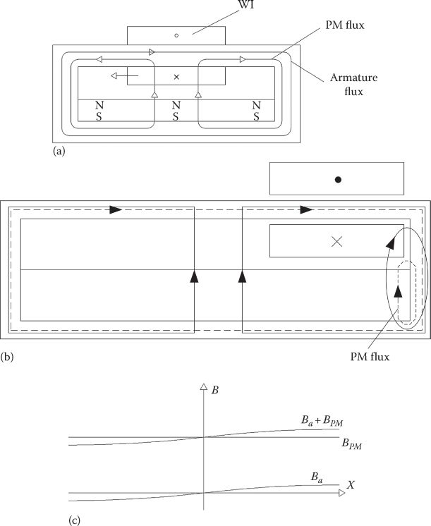
FIGURE 16.4 Flux lines and flux densities at (a) center position, (b) extreme position, and (c) force versus position at given current. (After Boldea, I. and Nasar, S.A., Linear Motion Electromagnetic Devices, Taylor & Francis, New York, 2001.)

On the other hand, the PM flux in the core right corner ϕ_c is

ϕ_{c} = B_{c \max} \cdot t_{c} \cdot w_{c} = B_{a} \cdot w_{c} \cdot t_{c} + B_{P M} \frac{(L_{s} + L_{c})}{2} w_{c} (16.3)

$ϕ_{c} = B_{c \max} \cdot t_{c} \cdot w_{c} = B_{a} \cdot w_{c} \cdot t_{c} + B_{P M} \frac{(L_{s} + L_{c})}{2} w_{c} (16.3)$

B_c_max in the core is limited by the core material B(H) curve and may be assessed by combining (16.2) and (16.3):

ϕ_{c \max} = w_{c} \cdot t_{c} \cdot B_{c \max} = [\frac{μ \cdot (B_{c}) \cdot N \cdot i}{2 (L_{s} + L_{c} + l_{s} + l_{p} + g + t_{c})} + B_{P M} \frac{(L_{s} + L_{c})}{2 \cdot t_{c}}] \cdot w_{c} \cdot t_{c} (16.4)

$ϕ_{c \max} = w_{c} \cdot t_{c} \cdot B_{c \max} = [\frac{μ \cdot (B_{c}) \cdot N \cdot i}{2 (L_{s} + L_{c} + l_{s} + l_{p} + g + t_{c})} + B_{P M} \frac{(L_{s} + L_{c})}{2 \cdot t_{c}}] \cdot w_{c} \cdot t_{c} (16.4)$

Equation 16.4 may be solved iteratively, if first

B_{P M} \approx B_{r} \cdot \frac{t_{p}}{t_{p} + g} \cdot \frac{1}{1 + K_{f r i n g e}} (16.5)

$B_{P M} \approx B_{r} \cdot \frac{t_{p}}{t_{p} + g} \cdot \frac{1}{1 + K_{f r i n g e}} (16.5)$

The fringe factor K_fringe depends on mover position to some extent (for start K_fringe = 0.1–0.2).

Equation 16.4 suggests that, for given B_c_max, for more force, more core area (w_ct_c) and more L_s + L_c (total length) are required. Conversely, if the length of travel L_s increases, by specifications, then, for more force, the core area (w_ct_c) should also increase.

The force per watt of copper losses is also to be considered. The ideal coil thickness (g = h_c + 2g_w) has to be smaller or equal to PM thickness to secure the highest force density:

h_{c} \approx g = \frac{N \cdot i_{n}}{L_{c} \cdot j_{c o n} \cdot K_{f i l l}} (16.6)

$h_{c} \approx g = \frac{N \cdot i_{n}}{L_{c} \cdot j_{c o n} \cdot K_{f i l l}} (16.6)$

K_fill is the copper fill factor

j_con is the design current density

The coil length l_coil is

l_{c o i l} \approx 2 (w_{c} + g) (16.7)

$l_{c o i l} \approx 2 (w_{c} + g) (16.7)$

and thus the coil resistance R_c is

R_{c} = \frac{1}{σ_{c o}} \frac{l_{c o i l}}{i_{n}} j_{c o n} \cdot N (16.8)

$R_{c} = \frac{1}{σ_{c o}} \frac{l_{c o i l}}{i_{n}} j_{c o n} \cdot N (16.8)$

σ_co is the copper electrical conductivity.

So the design copper losses p_con can be written as

p_{c o n} = \frac{2}{σ_{c o n}} (w_{c} + \frac{N \cdot i_{n}}{L_{c} \cdot j_{c o n} \cdot K_{f i l l}}) j_{c o n} \cdot N \cdot i_{n} (16.9)

$p_{c o n} = \frac{2}{σ_{c o n}} (w_{c} + \frac{N \cdot i_{n}}{L_{c} \cdot j_{c o n} \cdot K_{f i l l}}) j_{c o n} \cdot N \cdot i_{n} (16.9)$

Finally, the design force/watt of copper losses is

f_{x} = \frac{F_{x n}}{p_{c o n}} = \frac{B_{P M} \cdot σ_{c o}}{2 (1 + \frac{N \cdot i_{n}}{w_{c} \cdot L_{c} \cdot j_{c o n} \cdot K_{f i l l}}) j_{c o n}} (16.10)

$f_{x} = \frac{F_{x n}}{p_{c o n}} = \frac{B_{P M} \cdot σ_{c o}}{2 (1 + \frac{N \cdot i_{n}}{w_{c} \cdot L_{c} \cdot j_{c o n} \cdot K_{f i l l}}) j_{c o n}} (16.10)$

Now the PM flux in the coil Ψ_PM becomes

ψ_{P M} = N \cdot B_{P M} \cdot w_{c} \cdot x \cdot \frac{1}{1 + K_{f r i n g e} (x)} (16.11)

$ψ_{P M} = N \cdot B_{P M} \cdot w_{c} \cdot x \cdot \frac{1}{1 + K_{f r i n g e} (x)} (16.11)$

With K_fringe ≈ 0.1–0.2 ≈ const, x = 0 in the center position.

So the emf is

E = - \frac{d ψ_{P M}}{d x} \cdot \frac{d x}{d t} \approx \frac{- N \cdot B_{P M} \cdot w_{c}}{1 + K_{f r i n g e} (x)} \cdot u; u is the speed (16.12)

$E = - \frac{d ψ_{P M}}{d x} \cdot \frac{d x}{d t} \approx \frac{- N \cdot B_{P M} \cdot w_{c}}{1 + K_{f r i n g e} (x)} \cdot u; u is the speed (16.12)$

Finally, the coil inductance is

L_{c} \approx (1 + K_{l}) \frac{μ (i) \cdot N^{2} \cdot w_{c} \cdot t_{c}}{2 (L_{s} + L_{c} + l_{s} + t_{p} + g + t_{c})} (16.13)

$L_{c} \approx (1 + K_{l}) \frac{μ (i) \cdot N^{2} \cdot w_{c} \cdot t_{c}}{2 (L_{s} + L_{c} + l_{s} + t_{p} + g + t_{c})} (16.13)$

The core permeability μ(i) is an average one; in an analytical model, it may be a weighted average of three values in three key points of the core, while the actual magnetization curve B(H) of the core has to be considered. The factor K_l refers to the leakage inductance, which, in any case, is less than 0.2 even for, say, a soft magnetic composite core; not so for an air-core device.

Note on core losses: An analytical model of core losses may be obtained by refining the previously mentioned analytical model via the magnetic equivalent circuit model, where quite a few zones of uniform flux density variations have to be identified.

Then, by knowing the flux density variation in time, for the given linear motion profiles, the core loss may be calculated, by standard expressions, in each region; then they are added together.

Alternatively, 3D FEM may be used in magnetostatic mode, and then with the flux density/time variations in each finite element, the total core losses are calculated. For a tubular configuration, 2D FEM may be used directly, considering eddy current losses and even hysteresis losses [5].

16.4 Geometrical Optimization Design By FEM

For the configuration in Figure 16.1a, detailed, for the geometrical variables, in Figure 16.5, the optimization variables are obtained as L₁, L₂, L₃, L₄, and L₅. Two inequality constraints in mm [7] are visible in Figure 16.5:

\frac{2}{36} - 8 \cdot 8 \cdot L_{3} - \frac{L_{7}}{2} \geq 0.5 ††† 2 \cdot L_{3} + L_{5} \leq 36 (16.14)

$\frac{2}{36} - 8 \cdot 8 \cdot L_{3} - \frac{L_{7}}{2} \geq 0.5 ††† 2 \cdot L_{3} + L_{5} \leq 36 (16.14)$

A few equality constraints (specifications) are also given [7]:

Current density j_con = 24.5 A/mm²
Coil volume = 280 mm³
Mechanical gap G₁ = 0.4 mm (on one side of the coil)
G₂ = 0.5 mm—gap at the end of travel

With a given initial variable vector [L₁, L₂, L₃, L₄, L₅]^T, a 2D FEM (at least), and an optimization method, to change L_i in order to get maximum thrust, the optimization design is completed.

Images

FIGURE 16.5 Definition of geometrical design variables. (After Boldea, I. and Nasar, S.A., Linear Motion Electromagnetic Devices, Taylor & Francis, New York, 2001.)

We may augment the objective function by adding, say, temperature constraints, based on a simplified thermal model, etc.

In our case, with maximum force as the objective function, but also with given coil volume and current density, the copper losses are fixed. Therefore, in fact we are seeking here maximum thrust/watt of copper losses.

In Ref. [7], the Rosenbrock optimization method was used for the scope. The initial and final variable vectors are shown in Table 16.1 and the results are given in Table 16.2 [7].

The nonuniform distribution of force versus position is proven by FEM (Figure 16.6) but is not severe (Table 16.1).

During the 39 iterations (for a 0.01 mm convergence criterion), the variable vector was changed by a given step of 10% of initial values and the thrust was calculated by 2D FEM. If the thrust increased with respect to the previous step, the variables were changed by

\begin{array}{l} Δ L_{j}^{(k + 1)} = α L_{j}^{(k)}; α > 1.5 \\ otherwise, \\ Δ L_{j}^{(k + 1)} = - β L_{j}^{(k)}; β < 0.75 \end{array} (16.15)

$\begin{array}{l} Δ L_{j}^{(k + 1)} = α L_{j}^{(k)}; α > 1.5 \\ otherwise, \\ Δ L_{j}^{(k + 1)} = - β L_{j}^{(k)}; β < 0.75 \end{array} (16.15)$

TABLE 16.1
Dimensions of Initial and Final Shapes

Images

TABLE 16.2
Turns of Coil

	Thrust (N)
Position of Coil (mm)	Initial Shape	Optimal Shape	Ratio Increase (%)
−8.5	0.82	0.99	20
0	0.88	1.13	29
8.5	0.86	1.05	22

Images

FIGURE 16.6 Initial force versus position. (After Takahashi, S., Optimal design of linear dc motor using FEM, Record of LDIA-1995, Nagasaki, Japan, pp. 331–334, 1995.)

A 20% improvement in the thrust was obtained to reach 0.23 N/W [7], which is still modest, but the fixed current density was 24.5 A/mm² and the coil volume was 280 mm³.

16.5 Air-Core Configuration Design Aspects

For an optical disk drive application, the PM-in-air configuration (Figure 16.1b) was adopted [8]. A virtual path magnetic circuit model of the machine proved to compare acceptably with 3D FEM results (Figure 16.7), except for small airgap values. Even for this air-core machine, the PM flux density in the coil area is about 0.3 T.

The experimental results (Figure 16.8) for the mini linear dc PM motor of Table 16.3 [8] show a wide frequency response band, suitable for the application.

Images

FIGURE 16.7 Force versus airgap length between the two PMs. (After Park, J.H. et al., IEEE Trans., MAG-39(5), 3337, 2003.)

Images

FIGURE 16.8 Frequency response of the prototype. (After Park, J.H. et al., IEEE Trans., MAG-39(5), 3337, 2003.)

TABLE 16.3
Discretization Data

Number of elements	3.456
Number of nodes	1.741
Number of iterations of Rosenbrock’s method	39
CPU time (s)	201

16.6 Design for Given Dynamics Specifications

For the iron-core linear dc brushless PM motor, in a small power application (a digital video camera focuser), a more complicated optimal design should include not only the energy conversion ratio and the battery consumption but also the rising time (travel time for given travel length).

If the space is restricted to volume (l_x × l_y × l_z), Figure 16.9, we may end up with a few main variables [6]:

γ = \frac{l_{m}}{l_{w}} = \frac{P M thickness}{coil†thickness}; N = round (\frac{l_{w}}{ϕ}) \cdot round (\frac{l_{p}}{ϕ}) (16.16)

$γ = \frac{l_{m}}{l_{w}} = \frac{P M thickness}{coil†thickness}; N = round (\frac{l_{w}}{ϕ}) \cdot round (\frac{l_{p}}{ϕ}) (16.16)$

l_p is the coil length

ϕ is the coil conductor diameter

Images

FIGURE 16.9 Linear dc PM focuser for digital video camera. (After Yu, H.C. and Liu, T.S., IEEE Trans., MAG-43(11), 4048, 2007.)

The three performance indexes are then

Rising time t_r:

$d_{\max} = \int_{0}^{t_{r}} u d t (16.17)$ $d_{\max} = \int_{0}^{t_{r}} u d t (16.17)$

u is the speed

d_max is the travel length
Battery consumption (in J) E₀:

$E_{0} (γ, ϕ) = \int_{0}^{t_{r}} i (t) v (t) d t (16.18)$ $E_{0} (γ, ϕ) = \int_{0}^{t_{r}} i (t) v (t) d t (16.18)$
Energy efficiency:

$η_{e} (γ, ϕ) = \frac{E_{0} - \int_{0}^{t_{r}} i^{2} (t) \cdot R (γ, ϕ) d t}{E_{0}} (16.19)$ $η_{e} (γ, ϕ) = \frac{E_{0} - \int_{0}^{t_{r}} i^{2} (t) \cdot R (γ, ϕ) d t}{E_{0}} (16.19)$

All variables in (16.17) through (16.19) are functions of γ and ϕ; to use them in the optimization design, we have to solve for current i and speed u from voltage and motion equations:

\frac{d i}{d t} = \frac{v (t) - i (t) \cdot R (γ, ϕ) - K_{u} (γ, ϕ) \cdot u (t)}{L (γ, ϕ)} (16.20)

$\frac{d i}{d t} = \frac{v (t) - i (t) \cdot R (γ, ϕ) - K_{u} (γ, ϕ) \cdot u (t)}{L (γ, ϕ)} (16.20)$

\frac{d u}{d t} = \frac{K_{u} (γ, ϕ) \cdot i (t) - F_{l o a d} - B \cdot u (t)}{M} (16.21)

$\frac{d u}{d t} = \frac{K_{u} (γ, ϕ) \cdot i (t) - F_{l o a d} - B \cdot u (t)}{M} (16.21)$

where

L is the coil inductance

M is the mover mass

K_u is the emf (and force) constant (see Equation 16.11):

K_{u} (γ, ϕ) = \frac{d Ψ_{P M}}{d x} = \frac{F_{x}}{i} = K_{f} (16.22)

$K_{u} (γ, ϕ) = \frac{d Ψ_{P M}}{d x} = \frac{F_{x}}{i} = K_{f} (16.22)$

If the force F_x is calculated by 2D FEM, then K_u(γ, ϕ) may be determined from (16.22); also, the inductance L may be calculated from FEM, while the resistance R_c is

R_{c} = \frac{4}{σ_{c o}} \cdot \frac{N \cdot l_{c o i l} (γ)}{π ϕ^{2}} (16.23)

$R_{c} = \frac{4}{σ_{c o}} \cdot \frac{N \cdot l_{c o i l} (γ)}{π ϕ^{2}} (16.23)$

With the given voltage, R, L, K_f, K_u, B_m, d_max, and M and F_load, the three performance indexes may be calculated after solving for U and i in (16.20 and 16.21).

For M = 2 g, v = 3 V, i_max = 0.03 A, d_max = 5.2 mm, B_m = 0.005 N s/m, and F_load = 0.05 gw (gram weight), to compromise the three performance indexes finally [6], γ = 2.5, ϕ = 0.07 mm, for η_e = 4.9% (energy efficiency!), E₀ = 1.3 mJ, and rising time t_r = 44 ms [6]. This rising time is considered much better (6 times smaller) than that obtained with commercial rotary-stepper-plus transmission actuator. To fully characterize the design, R_c = 32.8 Ω, L = 1.2 mH, and K_u = K_f = 42.3 gw/A (measured) [6].

Though the energy efficiency η_e seems low, we have to consider it in comparison with existing solutions for such a small device.

16.7 Close-Loop Position Control for a Digital Video Camera Focuser

We are extending here the digital video camera focuser (Figure 16.9) analysis by dealing with the close-loop position control (open loop dynamics were investigated in the previous paragraph).

At this time, the voltage and motion equations parameters are as given previously.

The movable part is composed of the lens holder, the coil, and a linear magnetic strip mounted on a side tube. The stator includes the PMs, the yoke, a steel plate, and two motion-guiding pads. The position encoder includes the magnetoresistive (MR) sensor and a linear magnetic strip with 0.88 mm pole pitch; the final position estimation precision is around 3 μm. In addition, speed estimation is calculated from position feedback.

Two position control methods are used for comparison:

PID control
Sliding mode control

The PID control contains two cascaded loops, one for position and one for speed (Figure 16.10).

For sliding mode control, a sliding mode functional S(e), e = d* − d (position error) should be defined [9]:

S (e) = \ddot{e} + c_{2} \dot{e} + c_{3} e (16.24)

$S (e) = \ddot{e} + c_{2} \dot{e} + c_{3} e (16.24)$

If the sliding mode poles are p_1,2 = −α ± iβ, then

c_{2} = 2 α, c_{3} = {(α + β)}^{2} (16.25)

$c_{2} = 2 α, c_{3} = {(α + β)}^{2} (16.25)$

Images

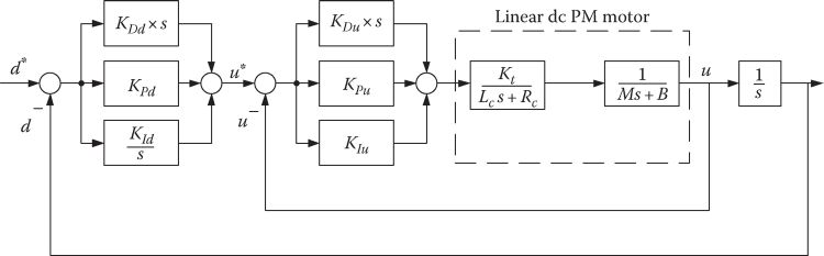
FIGURE 16.10 PID position control.

To be stable, the system has to stay close to the sliding mode surface S(e) = 0, but first to reach the sliding mode condition (surface)

S S < - σ (S); σ > 0 (16.26)

$S S < - σ (S); σ > 0 (16.26)$

To verify the stability and define a control law, the Lyapunov criterion is used, after a Lyapunov (energy) function V is chosen [9]:

V = S^{2} (16.27)

$V = S^{2} (16.27)$

But

\dot{V} = \frac{d V}{d t} = 2 S \dot{S} < - 2 σ (s) = - 2 σ \sqrt{V} < 0 (16.28)

$\dot{V} = \frac{d V}{d t} = 2 S \dot{S} < - 2 σ (s) = - 2 σ \sqrt{V} < 0 (16.28)$

As V > 0, V < 0 and thus the control will be asymmetrically stable if (16.26) is satisfied.

The control law may be defined, based on (16.24), as

U = - Q_{s a t} (s) - L_{3}^{- 1} c_{2} \ddot{e} - L_{3}^{- 1} c_{3} \dot{e} (16.29)

$U = - Q_{s a t} (s) - L_{3}^{- 1} c_{2} \ddot{e} - L_{3}^{- 1} c_{3} \dot{e} (16.29)$

With Q > 0, the maximum boundary of system states and disturbance is

S a t (S) = \begin{array}{l} s i g n (S); & i f | S | > ε \\ S / ε; & i f | S | \leq ε \end{array} (16.30)

$S a t (S) = \begin{array}{l} s i g n (S); & i f | S | > ε \\ S / ε; & i f | S | \leq ε \end{array} (16.30)$

Images

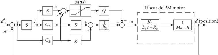
FIGURE 16.11 Sliding mode position control.

Images

FIGURE 16.12 Step position response: (a) in PID control and (b) by SM control. (After Yu, H.C. and Liu, T.S., IEEE Trans., MAG-43(11), 4048, 2007.)

The Sat function was used, instead of Sign function, to provide for low chattering response around the target. The close-loop control scheme is illustrated in Figure 16.11. The parameter Q may be adjusted based on minimization of error energy function $E n (e) = \int e^{2} d t$ $E n (e) = \int e^{2} d t$ .

It has to be noticed that

There is no cascaded control (as for PID control).
Quite a few position error time derivatives are required, but, as position is measured, the two derivatives may be obtained by adequate observers; also if an inertia accelerometer were made available, it would smooth notably the ė and ë observers (as done in MAGLEVs).

Sample results for the case in point, for PID and SM control, are given in Figure 16.12.

Both focusing time (from 120 to 60 ms) and steady-state precision (from 21 to 7 μm) are reduced for SM in comparison with PID control, as expected (SM control is known to provide fast and robust response with small overshooting).

16.8 Summary

The linear dc homopolar brushless PM motor has been developed from the voice-coil speaker microphone, but it develops control for progressive linear motion rather than oscillatory motion.
It is based on the Lorenz force and is essentially a single-phase linear synchronous brush-less PM motor with limited travel.
The practical travel length goes from a few mm to 100 mm or more.
Flat configurations with air core and iron core are typical for the linear dc brushless PM motor, while tubular ones are used in most speaker-microphone applications.
The Lorenz force sign changes with current polarity.
For limited travel, no brushes are required and the single (dual)-coil mover is fed from a flexible power cable.
The PM-mover configuration is feasible, but then the copper Joule loss in the stator coils is larger.
Iron-core configurations show higher force/volume while air-core configurations show slightly better force/weight but, also, higher frequency response band (due to lower electric time constant and inductance).
For iron-core flat configurations, analytical field model for circuit model parameters, and performance including magnetic saturation, produce satisfactory results for preliminary design purposes.
Secondary effects such as force reduction at travel ends may be ascertained properly with FEM analysis.
Force density and force/copper losses are two conflicting performance indexes that have to be reconciled in a proper design.
Core losses may be calculated by analytical or numerical field modes and are important when the duty cycle of back and forth motion is large.
For air-core topologies, virtual magnetic circuit models have been proven acceptable (validated by 3D FEM), except for a small distance between PMs (when two or three of them are provided); notable computer time is saved this way for optimization design.
Direct FEM geometrical optimization design has been successfully proven on linear dc brushless PM motors with 0.8 N force for 17 mm travel length at 0.23 N/W of copper losses as the objective function.
Direct FEM geometrical optimization may be exercised with some sophisticated performance indexes such as rising time, travel time per travel length, total energy consumption per rising time, and energy efficiency for the same. For a 2 g coil mover, a rising time of 44 ms, at total energy consumption of 1.3 mJ and energy efficiency of 4.9%, was obtained in view of focusing a digital video camera.
For the same application with given circuit parameters R = 32.8 O, L = 1.2 mH, K_u = K_f = 42.3 gw/A, and M = 1.8 g, both cascaded PID position and speed control and sliding mode (SM) position control have been investigated for a magnetostriction position sensor (5 µm in precision); SM control reduced the settling time for a 5 mm travel at 60 ms for a steady-state positioning precision of 7 µm, adequate for design video camera focusing; the existing rotary microstepper needs 400 ms for the same job.
Due to ruggedness, simplicity, and its rather long travel length, the linear dc brushless PM motor will find more and more applications when high-frequency band motion (in the hundreds of Hz range) is needed; the hot spots in R&D will perhaps be geometrical FEM, optimization design, and robust high-precision fast positioning control (For more, see Refs. [10,11]).

References

1. S.A. Nasar and I. Boldea, Linear Motion Electric Machines, John Wiley, New York, 1976.

2. A. Basak, Permanent Magnet Linear Dc Motors, Oxford University Press, 1996.

3. I. Boldea and S.A. Nasar, Linear Motion Electromagnetic Devices, Taylor & Francis, New York, 2001, Chapter 7.

4. H. Wakiwaka, H. Yajima, S. Senoh, and H. Yamada, Simplified thrust limit equation of linear Dc motor, IEEE Trans, MAG-32(5), 1996, 5073–5075.

5. M. Hippner, H. Yamada, and T. Mizuno, Iron losses in linear dc motor, IEEE Trans, MAG-38(5), 1999, 3715–3717.

6. H.-C. Yu, T.-Y. Lee, S.-J. Wang, M.-L. Lai, J.-J. Ju, D.-R. Huang, and S.-K. Lin, Design of a voice coil motor used in the focusing system of a digital video camera, IEEE Trans, MAG-41(10), 2005, 3979–3981.

7. S. Takahashi, Optimal design of linear dc motor using FEM, Record of LDIA-1995, Nagasaki, Japan, pp. 331–334.

8. J.H. Park, Y.S. Baek, and Y.P. Park, Design and analysis of mini-linear actuator for optical disk drive, IEEE Trans, MAG-39(5), 2003, 3337–3339.

9. H.C. Yu and T.S. Liu, Output feedback sliding mode control for a linear focusing actuator in digital video cameras, IEEE Trans, MAG-43(11), 2007, 4048–4050.

10. P. Fang, F. Ding, Q. Li, and Y. Li, High response electromagnetic actuator with twisting axis for gravure systems, IEEE Trans, MAG-45(1), 2009, 172–175.

11. C.-S. Liu, P.-D. Lin, S.-S. Ke, Y.-H. Chang, and J.-B. Horng, Design and characterization of miniature auto focusing voice coil motor actuator for cell-phone camera applications, IEEE Trans, MAG-45(1), 2009, 155–159.

..................Content has been hidden....................

You can't read the all page of ebook, please click here login for view all page.

Table of Contents for
Chapter 16 Linear DC PM Brushless Motors

16 Linear DC PM Brushless Motors

16.1 Introduction

16.2 Topology Aspects

16.3 Principle and Analytical Modeling

16.4 Geometrical Optimization Design By FEM

16.5 Air-Core Configuration Design Aspects

16.6 Design for Given Dynamics Specifications

16.7 Close-Loop Position Control for a Digital Video Camera Focuser

16.8 Summary

References

Table of Contents for Chapter 16 Linear DC PM Brushless Motors

Create new playlist

Sign In

Sign Up

Table of Contents for
Chapter 16 Linear DC PM Brushless Motors