Chapter 3 Linear Induction Motors: Topologies, Fields, Forces, and Powers Including Edge, End, and Skin Effects

Search in book...
Toggle Font Controls
Create new playlist

Name your new playlist

Playlist description (optional)
Sign In

Email address

Password

Forgot Password?

or

Continue with Facebook

Continue with Google
Sign Up

Full Name

Email address

Confirm Email Address

Password

or

Continue with Facebook

Continue with Google

Topologies, Fields, Forces, and Powers Including Edge, End, and Skin Effects

This chapter deals with flat linear induction motor (LIM) topologies, double sided and single sided, with their windings and field technical theories accounting for edge, longitudinal end, and skin effects, with the scope of providing a deep understanding of flat LIMs performance and limitations and, also, preparing analytical expressions for equivalent circuit models of LIMs to be developed and then used to investigate the dynamics and control of LIMs (Chapter 4).

3.1 Topologies of Practical Interest

As seen in Chapter 2, LIMs are counterparts of rotary induction motors. They may be obtained by “cutting” and unrolling the rotary induction machines to yield flat, single-sided topologies (Figure 3.1a), where the cage secondary may be used as such or replaced by an aluminum sheet placed between two primaries to make the double-sided LIM (Figure 3.1b).

The passive long secondary (track) is fixed for short-primary-mover configurations (Figure 3.1) and secures a reasonable low cost track/km, while it imposes transfer of full propulsion electric power on board of vehicle, together with the static power converters and their control. However, the vehicle becomes independent, and a faulty vehicle may be put away to let the track available for the healthy vehicles.

Though the research on LIMs has started with double-sided configurations, it ended up so far in using single-sided moving primary topologies for transportation (on wheels or on magnetic suspension) in commercial applications. For long tracks, an aluminum sheet on solid mild iron (made of 3–4 “thick” laminations) secondary (Figure 3.1c) may be preferable on account of lower cost, at the price of lower LIM efficiency and power factor, with corresponding consequences in increased inverter kVA ratings and costs.

The ladder secondary allows for a lower (up to 10–12 mm) magnetic airgap (in transportation) than the aluminum sheet on iron secondary (16–18 mm). The double-sided LIM implies for transportation applications a total magnetic airgap of 26–40 mm, which, unless the pole pitch is high, leads to small power factors (less than 0.4).

Besides propulsion force (thrust) F_x, normal force F_n is exerted on the LIM primary. But for double-sided LIM (Figure 3.1b), the net normal force on secondary is zero for symmetrical position of the latter in the airgap. On the contrary, the single-sided LIM is characterized by a net nonzero normal force (on secondary and primary)—F_n/F_x ≈ 3–4—which may be used for active magnetic suspension by adequate control in MAGLEVs. The normal force is notably higher for ladder secondary single-sided LIMs (F_n/F_x ≈ 8–10), providing perhaps all necessary magnetic suspension for an acceleration of 1 m/s in vehicles where the LIMs represent 10% of loaded vehicle weight.

Images

FIGURE 3.1 LIM flat topologies with short-primary mover: (a) single-sided with cage-core secondary (track), (b) double-sided with aluminum-strip secondary (track), and (c) single-sided with aluminum sheet on iron secondary.

For the double-sided LIM (DLIM), with close to zero normal force, separate dc-fed controlled electromagnets acting on a separate solid iron track are required for active magnetic suspension in LIM-MAGLEVs.

There are also tubular LIMs—as introduced in Chapter 2—but they are destined to low excursion (lower than 1.5–2 m) and will be treated separately in Chapters 4 and 5 as low-speed LIMs.

Long-primary active track with wound-secondary short movers have also been proposed [1], but the development of synchronous long-primary (active guideway) linear motors with superior performance (due to dc mover magnetization) has rendered them less practical.

Considering flat, double-sided, and single-sided short-primary LIMs, we should notice that their cores are to be laminated (even coarsely) as in rotary IMs. The LIM short-primary cores are open magnetic circuits along the direction of motion, and thus the three-phase ac windings located in their uniform slots have special peculiarities, though their purpose is the same as in rotary IMs: to produce traveling magnetomotive forces (mmfs) and thus close to traveling airgap magnetic flux density. Basically, there are two main types of LIM practical windings:

Single-layer 2p (even) pole windings (Figure 3.2a)
Double-layer 2p + 1 (odd) pole windings with half-filled end slots (Figure 3.2b)

While Figure 3.2 illustrates q₁ = 1 slot/pole/phase, full-pitch-coil three-phase LIM windings, for large (transportation) LIMs, q₁ = 2,3 and short span coils (for two-layer windings) may be used to produce closer to traveling mmf, as in rotary IMs (with lower space harmonics).

As the power factor of LIMs, due to larger airgap/pole pitch ratios than in rotary IMs, tends to be lower, the magnetization current in p.u. tends to be larger—around or even higher than Irated/2–√ $I_{r a t e d} / \sqrt{2}$ —and thus, if end-turns relative length (dependent on l_stack/pole pitch) tends to be large in some applications, the two-layer chorded-coil windings are to be preferred as their end turns are shorter (10%–20%).

To further shorten the end-turns length, some peculiar windings such as those in Figure 3.3 may be adopted.

The three-layer winding with chorded coils (Figure 3.3a) provides a 0.867 fundamental winding factor and uses the primary slots less efficiently but shows notable shorter end coils while, however, the phase resistance and self and mutual inductances are slightly nonsymmetric. The tooth-coil winding in Figure 3.3b has q = 1/2 slots/pole and phase and poor fundamental winding factor, but it shows very short end connections.

Finally, the tooth-coil winding in Figure 3.3c, with 12 coils, in a different connection can produce a 10-pole mmf, with a good fundamental winding factor (around 0.933), but not all 10 poles are symmetric. Two such primaries, phase shifted properly, could improve the 10-pole mmf symmetry and be satisfactory for some applications, though higher order space harmonics still show up in the mmf, in a double-sided primary LIM configuration.

The winding in Figure 3.3c is typical for linear PM synchronous motors, as it is easy to manufacture and the end coil length is low; they have a high fundamental winding factor. The fundamental winding factor is the ratio between real emf and its ideal value when the emf in all coils in series per phase would add arithmetically. Reducing the subharmonics in tooth-coil (fractionary) windings with N_s1 and 2p slightly different from each other may be tried by dividing some of the slot volume into 2, 3 coils of different phases. The ac windings so far are three phase, but split-phase (or two-phase) windings may also be envisaged for small thrust (power) applications as for rotary IMs. Two-phase symmetric windings may be preferable when 2p = 2, 4 in low-speed applications to avoid phase current asymmetry.

The topologies of practical interest so far warrant remarks as follows:

The magnetic airgap (g_m) is larger than the mechanical airgap (g) in DLIMs and in single-sided LIMs with conductive sheet on iron secondary thickness:

$g m = K \times g + h A L (3.1)$ $g_{m} = K \times g 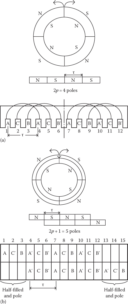+ h_{A L} (3.1)$

FIGURE 3.2 Single- and two-layer three-phase LIM windings: (a) 2p = 4, q₁ = 1 slot/pole/phase, single layer; (b) 2p + 1 = 5, q₁ = 1, double layer.

K = 1 for single-sided LIM (SLIM) and K = 2 for DLIM.

The magnetic circuit of LIMs is open along the direction of motion (it has limited length); however, the Gauss flux law applies, so there may be a redistribution of airgap in the back-iron (yoke) flux densities, in contrast to rotary IMs where circumferentially the magnetic circuit is closed.

FIGURE 3.3 Short end-coil LIM windings: (a) N_C = 12, 2p = 4, q₁ = 1, y/τ = 2/3, 3 layers and (b) N_C = 12, 2p = 4, q₁ = 1/2, y/τ = 1/3—tooth coils; (c) N_s1 = 12, 2p = 10, q = 2/5.
The primary mmf fundamental may be described by a traveling wave, along the primary length, as in rotary IMs [2]:

$θ (x, t) = θ m 1 \cdot cos (ω 1 \cdot t - π τ x), for 0 < x < 2 p τ (3.2)$ $θ (x, t) = θ_{m 1} \cdot \cos (ω_{1} \cdot t - \frac{π}{τ} x), for 0 < x < 2 p τ (3.2)$

$θ (x, t) = 0 for x < 0 and x > 2 p τ$ $θ (x, t) = 0 for x < 0 and x > 2 p τ$

$F m 1 = 3 2 - \sqrt \cdot W 1 \cdot I 1 \cdot k ω 1 π p (3.3)$ $F_{m 1} = \frac{3 \sqrt{2} \cdot W_{1} \cdot I_{1} \cdot k_{ω_{1}}}{π p} (3.3)$

where

p is pole pairs

W₁ is turns per phase in series (for one current path only)

ω₁ = 2 • π • f₁, f₁ is the primary frequency, τ is the pole pitch or half the period of primary mmf wave, I₁ is the rms value of primary phase current

Formulae (3.2) through (3.3) are valid strictly for a 2p (even) pole-count windings (Figure 3.2a).
For the 2p + 1 (odd) pole winding, we may consider two such waves, halved in amplitude and phased shifted by τ in space and by 180° in time (Figure 3.2b) for full pitch coils; for chorded coils, the space shift is less than τ

$θ (x, t) = θ x u (x, t) + θ x l (x, t) (3.4)$ $θ (x, t) = θ_{x u} (x, t) + θ_{x l} (x, t) (3.4)$

$θ x u (x, t) = F m 1 2 \cdot cos (ω 1 \cdot t - π τ \cdot x) for 0 < x \leq 2 p τ (3.5)$ $θ_{x u} (x, t) = \frac{F_{m 1}}{2} \cdot cos (ω_{1} \cdot t - \frac{π}{τ} \cdot x) for 0 < x \leq 2 p τ (3.5)$

$θ x u (x, t) = 0 for 0 > x and x > 2 p τ (3.6)$ $θ_{x u} (x, t) = 0 for 0 > x and x > 2 p τ (3.6)$

$θ x l (x, t) = - θ m 1 2 \cdot cos (ω 1 \cdot t - π τ \cdot x) for τ \leq x \leq (2 p + 1) \cdot τ (3.7)$ $θ_{x l} (x, t) = - \frac{θ_{m 1}}{2} \cdot \cos (ω_{1} \cdot t - \frac{π}{τ} \cdot x) for τ \leq x \leq (2 p + 1) \cdot τ (3.7)$

$θ x u (x, t) = 0 for τ > x and x > (2 p + 1) \cdot τ (3.8)$ $θ_{x u} (x, t) = 0 for τ > x and x > (2 p + 1) \cdot τ (3.8)$
One of the three windings is placed in a different position with respect to the open core end (phase c) and thus, at least for low number of poles 2p = 2, 4, 6 or 5, 7, we expect slightly different self and mutual inductances of the phases, which translates into asymmetric phase currents for symmetric supply voltages. Even if symmetric current control is performed through a PWM inverter, the different self and mutual inductances will trigger slight thrust pulsations. This effect, present from zero speed, may be called static end effect. In a multiple unit, we may envisage three primary modules where the order of phases in slots is “rotated” and thus, for their series connection phase by phase, the phase currents will become symmetric; also, the total thrust pulsations are reduced.

It may be argued that by adopting a symmetric two-phase winding with 2p = 2, 4, the phase currents will be symmetric and thus the static end effect is zero; true, but we need a two-phase dedicated inverter, which shows a smaller number of nonzero voltage vectors and thus higher current ripple is expected. Even so, for 2p = 2, 4 poles in small thrust applications, the two-phase winding seems the first option, which justifies building a dedicated two-phase inverter and control system.
As is well known, the back-iron flux, in the primary and secondary of rotary IMs, is half the airgap pole flux Φ_1p:

$Φ y s = Φ 1 p 2 (3.9)$ $Φ_{y s} = \frac{Φ_{1 p}}{2} (3.9)$

For LIMs, the maximum back-iron flux becomes larger, up to almost equal to the pole flux (airgap flux per pole) due to airgap flux redistribution to suit Gauss flux law over the limited core longitudinal extension of primary:

$B g 1 (x, t) = μ 0 \cdot F m 1 \cdot cos ( ω 1 \cdot t - π τ \cdot x ) K C \cdot g m \cdot ( 1 + k s ) (3.10)$ $B_{g 1} (x, t) = \frac{μ_{0} \cdot F_{m 1} \cdot \cos (ω_{1} \cdot t - \frac{π}{τ} \cdot x)}{K_{C} \cdot g_{m} \cdot (1 + k_{s})} (3.10)$

$B y s (x, t) = 1 h y s \cdot \int 0 x B g 1 (x, t) = B g 1 \cdot τ π \cdot h y s \cdot (sin (ω 1 \cdot t) - sin (ω 1 \cdot t - π τ \cdot c)) (3.11)$ $B_{y s} (x, t) = \frac{1}{h_{y s}} \cdot \int_{0}^{x} B_{g 1} (x, t) = \frac{B_{g 1} \cdot τ}{π \cdot h_{y s}} \cdot (\sin (ω_{1} \cdot t) - \sin (ω_{1} \cdot t - \frac{π}{τ} \cdot c)) (3.11)$

FIGURE 3.4 DLIM, zero secondary conductivity (ideal no load) flux lines produced by primary traveling mmf (2p = 4 poles).

Even for a pure traveling airgap flux density, which, for zero secondary conductivity, fulfills Gauss flux law, the back-iron flux density B_ys has an additional component, and thus for x = τ, 3τ, 5τ, B_ys is B_ysmax = (2 • B_g1 • τ)/(π • h_ys) instead of (B_g1 • τ)/(π • h_ys) as in rotary LMs.

Figure 3.4 illustrates the fact that the total flux per end pole is forced to flow through the back iron as its flux lines do not close through the air zones outside the primary (longitudinal core ends). A similar assertion is valid for the central poles of the 2p + 1 pole primaries.
The almost doubling of back-iron flux density in some points in comparison with rotary LIM has notable design consequences in low-pole-count LIMs (2p = 2, 4 or 2p + 1 = 5) in the sense of doubling the back-iron depth for given flux density in the primary; for the single-sided LIM, the solid back iron of the secondary has to handle also almost all pole flux, which means a much higher degree of magnetic saturation and skin effects, to be considered in any realistic design.

As the maximum yoke flux density appears at x = 3τ, 5τ, it suggests avoiding drawing holes in those regions for stacking the laminations or cooling, etc.

3.2 Specific LIM Phenomena

3.2.1 Skin Effect

The secondary frequency f₂ of the secondary emfs and their currents may be calculated as a function of slip S, as for the rotary IMs:

f 2 = S \cdot f 1 (3.12)

$f_{2} = S \cdot f_{1} (3.12)$

with

S = ( U s - U ) U s; U s = 2 τ f 1 (3.13)

$S = \frac{(U_{s} - U)}{U_{s}}; U_{s} = 2 τ f_{1} (3.13)$

The ideal synchronous speed U_s (or the mmf wave speed) is, as for rotary IMs, U_s = 2 • τ • f₁, where U is the linear speed opposite to U_s, in short (moving) primary LIMs.

As, in general, the thickness of the secondary conductive sheet is rather small, to reduce long secondary (track) costs, with respect to primary slot depth, there is a need for a rather large slip, 5%–10%, to produce notable thrust density (1–2 N/cm² of primary area). In a DLIM, the aluminum secondary thickness (per primary side) h_AL/2 is up to about 6–8 mm for large high-speed LIMs and so is h_AL for SLIM with aluminum sheet on iron secondary.

The depth of ac field penetration in a conductor δ_AL is [2]

δ A L = 2 S \cdot 2 π \cdot f 1 \cdot μ 0 \cdot σ A L - - - - - - - - - - - - - - - - \sqrt (3.14)

$δ_{A L} = \sqrt{\frac{2}{S \cdot 2 π \cdot f_{1} \cdot μ_{0} \cdot σ_{A L}}} (3.14)$

where σ_AL is the aluminum conductivity.

For S • f₁ = 10 Hz, σ_AL = 3.33 × 10⁷ Ω⁻¹ m⁻¹, δ_AL = 0.0276 m.

As δ_AL at 10 Hz is notably larger than the thickness of aluminum plate (sheet), the skin effect is not very important (as known from rotary IMs; K_R ≈ 1 + ξ= 1 + h_AL/δ_AL, because h_AL/δ_AL ≪ 1).

The depth of field penetration may be corrected by considering the traveling field (and not the ac field characteristic to rotary IM slots) variation with x in a simplified bidimensional airgap field model where δ_AL would be replaced by δ′_AL:

δ' A L = Re ⎛ ⎝ ⎜ 1 ( π / τ ) 2 + j \cdot S \cdot f 1 \cdot 2 π \cdot μ 0 \cdot σ A L - - - - - - - - - - - - - - - - - - - - - - - - \sqrt ⎞ ⎠ ⎟ (3.15)

${δ^{'}}_{A L} = Re (\frac{1}{\sqrt{{(π / τ)}^{2} + j \cdot S \cdot f_{1} \cdot 2π \cdot μ_{0} \cdot σ_{A L}}}) (3.15)$

For high pole pitches (τ > 0.1 m) the first term under the square root in (3.15) is rather small but it may still be considered, for a few percent better precision. Now the aluminum skin effect coefficient K_{R skin} of rotary IMs may be applied [2]:

K R s k i n = ξ sinh ( 2 ξ ) + sin ( 2 ξ ) cosh ( 2 ξ ) - cos ( 2 ξ ) (3.16)

$K_{R s k i n} = ξ \frac{\sinh (2ξ) + \sin (2ξ)}{\cosh (2ξ) - \cos (2ξ)} (3.16)$

ξ = h A L δ ' A L (3.17)

$ξ = \frac{h_{A L}}{{δ^{'}}_{A L}} (3.17)$

In essence, the current density crowds closer to the aluminum sheet surface, perpendicular to the airgap normal flux density: its phase is also shifted along the aluminum sheet depth. The h_AL is replaced by h_AL/2 for the DLIM in (3.16) because the magnetic field penetrates the aluminum sheet from both sides (Figure 3.5).

If the SLIM secondary back iron is solid, its field depth of penetration at f₂=S • f₁ is notably smaller unless the latter gets heavily saturated:

δ' i r o n = Re ⎛ ⎝ ⎜ 1 ( π / τ ) 2 + j \cdot S \cdot f 1 \cdot 2 π \cdot μ ( B t i r o n ) \cdot σ i r o n - - - - - - - - - - - - - - - - - - - - - - - - - - - - - - \sqrt ⎞ ⎠ ⎟ (3.18)

${δ^{'}}_{i r o n} = Re (\frac{1}{\sqrt{{(π / τ)}^{2} + j \cdot S \cdot f_{1} \cdot 2 π \cdot μ (B_{t i r o n}) \cdot σ_{i r o n}}}) (3.18)$

For same S • f₁ = 10 Hz, τ = 0.15 m, and σ_iron=3.5 × 10⁶ (Ω m)⁻¹, even with μ_iron = 60 • μ₀ (at B_{t iron} ≈ 2 T, H_iron = 26,540 A/m), δ′_iron = 11 mm.

B_t is the tangential flux density on the back-iron upper surface.

Images

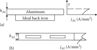
FIGURE 3.5 Current density amplitude variation in aluminum versus aluminum sheet thickness: (a) SLIM and (b) DLIM.

As the approximate back-iron flux is about the flux per pole, we have

B t m a x \cdot δ' i r o n (1 - e - 1) \approx B g 1 \cdot 2 π \cdot τ (3.19)

$B_{t m a x} \cdot {δ^{'}}_{i r o n} (1 - e^{- 1}) \approx B_{g 1} \cdot \frac{2}{π} \cdot τ (3.19)$

Consequently, B_g1, B_{t max} • δ′_iron (1 − e⁻¹), the peak airgap flux density is B_g1 = 0.209 T. This is a rather small value. Consequently, the back iron should be divided into a few (3–4) sections or “laminations” (Figure 3.6) so as to reduce the effective electric conductivity of iron and thus increase the field penetration depth to 20 mm or more and to provide for a load airgap flux density of at least 0.4 T.

Note: For ladder secondary, if the secondary iron core is laminated, the skin effect has to be treated as in rotary IMs [2]. This rationale leads to the conclusion that the skin effect produces a decrease in the equivalent conductivity σ_e = σ/K_{R skin}. The secondary leakage inductance as a consequence of skin effect (due to secondary iron eddy current density phase shifting, along iron depth) may be neglected for DLIMs but not for SLIMs.

3.2.2 Large Airgap Fringing

At least in transportation applications, the magnetic airgap g_m per pole pitch τ ratio is rather large in comparison with rotary IMs. In a simplified 2 • D(x, y) field theory, the traveling mmf varying with ej⋅πτ⋅x $e^{j \cdot \frac{π}{τ} \cdot x}$ will lead to a vertical (along z) variation with sinh(π/τ)y and cosh(π/τ)y. In essence, the equivalent airgap is approximately increased to g_mec = g_m • K_Fg, [3–7]:

K F g \approx sinh ( π / τ ) \cdot g m ( π / τ ) \cdot g m \geq 1 (3.20)

$K_{F g} \approx \frac{\sinh (π / τ) \cdot g_{m}}{(π / τ) \cdot g_{m}} \geq 1 (3.20)$

A typical 2D field distribution of airgap flux lines for a DLIM is shown in Figure 3.6, where both skin effect and large airgap fringing are visible.

Images

FIGURE 3.6 2D airgap field in DLIM under load (with aluminum sheet currents). (After Nasar, S.A. and Boldea, I., Linear Motion Electromagnetic Devices, Taylor & Francis, New York, 2001.)

3.2.3 Primary Slot Opening Influence on Equivalent Magnetic Airgap

The airgap flux density is modulated by the primary slot openings (Figure 3.7a); an equivalent effect consists of a larger constant airgap g_e.

The ratio g_mec/g_m = K_C (K_C = 1.1–1.7 in general), Carter coefficient, a one-century-old concept, revised recently for large magnetic airgap (PM) machines, puts face to face the old and a newly derived formula [5]—both obtained by conformal mapping:

K c = g m e c g m = 1 1 - σ c \cdot b s τ s; τ s; slot pitch (3.21)

$K_{c} = \frac{g_{m e c}}{g_{m}} = \frac{1}{1 - σ_{c} \cdot \frac{b_{s}}{τ_{s}}}; τ_{s}; slot pitch (3.21)$

σ c = 2 π \cdot tan - 1 (b s 2 \cdot g m) - 1 π \cdot 2 \cdot g m b s \cdot ln ((1 + b s 2 \cdot g m) 2) (3.22)

$σ_{c} = \frac{2}{π} \cdot \tan^{- 1} (\frac{b_{s}}{2 \cdot g_{m}}) - \frac{1}{π} \cdot \frac{2 \cdot g_{m}}{b_{s}} \cdot \ln ({(1 + \frac{b_{s}}{2 \cdot g_{m}})}^{2}) (3.22)$

and

K c n e w = 1 + τ s 2 π g m [(1 + α) \cdot log (1 + α) + (1 - α) \cdot log (1 - α)] (3.23)

$K_{c n e w} = 1 + \frac{τ_{s}}{2 π g_{m}} [(1 + α) \cdot \log (1 + α) + (1 - α) \cdot \log (1 - α)] (3.23)$

α = b s τ s; b s, slot opening

$α = \frac{b_{s}}{τ_{s}}; b_{s}, slot opening$

Reference [5] establishes regions where one or the other formula is preferable (Figure 3.7) but, in general, for large g_m/τ_s and b_s/τ_s values, the new formula (3.23) is more precise.

If the magnetic airgap g_m= g + h_AL is large (14–30 mm), then the slots may be open, as long as b_s < 2 • g_m, which leads to easy insertion of coils in slots, while K_c is, in general, less than 1.15. For low (0.7–1.2 mm) mechanical airgap (industrial, short-travel machine tool table applications), the ladder secondary is preferable, as it leads to satisfactory efficiency and power factor (both above 0.7) even at speeds below 3 m/s. In such cases, semiclosed slots, at least in the primary, are to be used.

3.2.4 Edge Effects

For the aluminum sheet or aluminum sheet on iron secondaries of LIM, the trajectory of induced secondary currents (by the traveling stator mmf) is closed (div J¯¯=0 $\bar{J} = 0$ )—Figure 3.8—and thus a 2D field analysis is required to portray them; only the transverse (J_y) component produces thrust, with J_x producing, in the active zone, only additional losses. Active zone is the one between the primaries (in DLIMs) and between primary and secondary back iron (in SLIMs). The laterally outside zone corresponds to the “end-ring” zone in rotary IMs.

The effect of the presence of J_x in the active zone is called edge effect. It boils down to a decrease in conductive sheet equivalent electrical conductivity K_tR, which is dependent on machine geometry and secondary (slip) frequency f₂ = S • f₁ in DLIM and, in addition, on magnetic saturation in SLIM. There is also a very small decrease in the magnetization inductance due to edge effect, but this may be neglected in most practical cases. (This phenomenon is absent in ladder secondary SLIMs.) We will rederive here in short the 2D field analysis of edge effects for DLIMs and then generalize it to SLIMs.

Images

FIGURE 3.7 Slot opening influence on airgap flux density (Carter coefficient): (a) airgap flux density waveform; (b) Carter coefficient formulae: dividing regions. (After Matagne, E., Electromotion, 15(4), 171, 2008.)

To separate the edge effect in a 2D field analysis, let us assume that

The two primaries slotting is replaced by an increased airgap via K_C > 1
The airgap fringing is accounted for by K_Fg > 1
So the total equivalent airgap g_et = g_m • K_C • K_Fg
The stator mmf is represented by its fundamental traveling wave in secondary coordinates

$θ 1 (x, t) = F 1 m \cdot e - j \cdot (S \cdot ω 1 \cdot t - π τ \cdot x) (3.24)$ $θ_{1} (x, t) = F_{1 m} \cdot e^{- j \cdot (S \cdot ω_{1} \cdot t - \frac{π}{τ} \cdot x)} (3.24)$
S • ω₁ is the secondary angular frequency of induced currents
We may separate the time dependence as the secondary current density varies sinusoidally in time with secondary (slip) frequency S • ω₁
The LIM length is so large along motion direction that there is no end effect (to be treated later in this chapter)

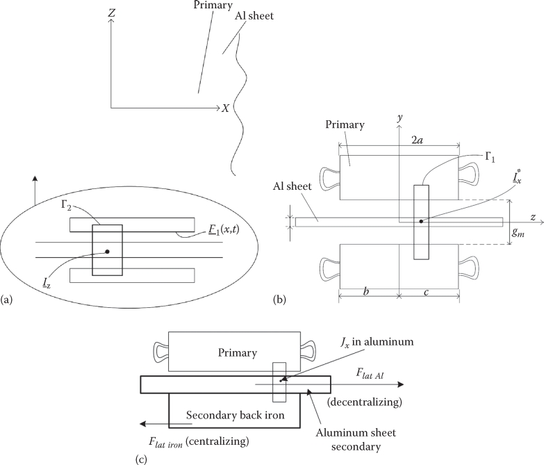
FIGURE 3.8 (a) Secondary current density components, (b) DLIM cross-section, and (c) decentralized SLIM secondary.
Outside the active zone (lyl > a_e, a_e ≈ a + g_et), g_et is introduced to account for transversal flux fringing), as div J¯¯2=0 ${\bar{J}}_{2} = 0$ :

$\partial J 2 x \partial x + \partial J z \partial z = 0 (3.25)$ $\frac{\partial J_{2 x}}{\partial x} + \frac{\partial J_{z}}{\partial z} = 0 (3.25)$
At y = −b, c, as expected, and J_z = 0
Inside the active zone, we apply Ampere’s law along contours Γ₁ and Γ₂ in Figure 3.8:

$g e t \cdot \partial H y \partial z = J 2 x \cdot d A L (3.26)$ $g_{e t} \cdot \frac{\partial H_{y}}{\partial z} = J_{2 x} \cdot d_{A L} (3.26)$

$- g e t \cdot \partial ( H y + H 0 ) \partial x = J m + J 2 z \cdot d A L (3.27)$ $- g_{e t} \cdot \frac{\partial (H_{y} + H_{0})}{\partial x} = J_{m} + J_{2 z} \cdot d_{A L} (3.27)$

where H_y is the only magnetic field component, produced by the secondary currents, while H₀ is the initial airgap field in the absence of secondary currents; J_m is the primary current sheet (in A turns/m):

J ¯ ¯ m = \partial θ ¯ 1 ( x , t ) \partial x (3.28)

${\underline{J}}_{m} = \frac{\partial {\underline{θ}}_{1} (x, t)}{\partial x} (3.28)$

Adding Faraday’s law,

\partial J 2 z \partial z - \partial J 2 x \partial z = - j \cdot S \cdot ω 1 \cdot μ 0 \cdot σ e t \cdot (H y + H 0) (3.29)

$\frac{\partial J_{2 z}}{\partial z} - \frac{\partial J_{2 x}}{\partial z} = - j \cdot S \cdot ω_{1} \cdot μ_{0} \cdot σ_{e t} \cdot (H_{y} + H_{0}) (3.29)$

σ_et= σ/K_{R skin}, accounts for the skin effect in the secondary ((3.16), with d_AL/2 instead of d_AL for DLIM).

H₀ is obtained from (3.27) with J_2z = 0:

H 0 = j \cdot J m \cdot e - j \cdot π τ \cdot x ( π / τ ) \cdot g e t (3.30)

$H_{0} = \frac{j \cdot J_{m} \cdot e^{- j \cdot \frac{π}{τ} \cdot x}}{(π / τ) \cdot g_{e t}} (3.30)$

Equations 3.26 through 3.29 lead to the equation of magnetic field of secondary currents (H_y):

\partial 2 H y \partial x 2 + \partial 2 H y \partial x 2 - j \cdot S \cdot ω 1 \cdot σ e t \cdot μ 0 d A L g e t \cdot H y = j \cdot S \cdot ω 1 \cdot σ e t \cdot μ 0 d A L g e t \cdot H 0 (3.31)

$\frac{\partial^{2} H_{y}}{\partial x^{2}} + \frac{\partial^{2} H_{y}}{\partial x^{2}} - j \cdot S \cdot ω_{1} \cdot σ_{e t} \cdot μ_{0} \frac{d_{A L}}{g_{e t}} \cdot H_{y} = j \cdot S \cdot ω_{1} \cdot σ_{e t} \cdot μ_{0} \frac{d_{A L}}{g_{e t}} \cdot H_{0} (3.31)$

Equation 3.31 is valid for |z| < a_e, that is, in the active zone.

The solution of (3.31) is straightforward:

H y = - H 0 \cdot ( j \cdot S \cdot ω 1 \cdot μ 0 \cdot σ e t \cdot d A L / g e t ) ( ( π 2 / τ 2 ) + j \cdot S \cdot ω 1 \cdot σ e t \cdot μ 0 ( d A L / g e t ) ) + A \cdot cosh (α \cdot z) + B \cdot sinh (α \cdot z) (3.32)

$H_{y} = \frac{- H_{0} \cdot (j \cdot S \cdot ω_{1} \cdot μ_{0} \cdot σ_{e t} \cdot d_{A L} / g_{e t})}{((π^{2} / τ^{2}) + j \cdot S \cdot ω_{1} \cdot σ_{e t} \cdot μ_{0} (d_{A L} / g_{e t}))} + A \cdot \cosh (α \cdot z) + B \cdot \sinh (α \cdot z) (3.32)$

with

α 2 = π 2 τ 2 + j \cdot ω 1 \cdot S \cdot μ 0 \cdot σ e t d A L g e t = (π τ) 2 \cdot (1 + j \cdot S \cdot G e t) (3.33)

$α^{2} = \frac{π^{2}}{τ^{2}} + j \cdot ω_{1} \cdot S \cdot μ_{0} \cdot σ_{e t} \frac{d_{A L}}{g_{e t}} = {(\frac{π}{τ})}^{2} \cdot (1 + j \cdot S \cdot G_{e t}) (3.33)$

If we define by G_et,

G e t = μ 0 \cdot τ 2 \cdot ω 1 π 2 \cdot σ e t \cdot d A L g e t (3.34)

$G_{e t} = \frac{μ_{0} \cdot τ^{2} \cdot ω_{1}}{π^{2}} \cdot σ_{e t} \cdot \frac{d_{A L}}{g_{e t}} (3.34)$

Then,

H y = - H 0 \cdot ( j \cdot S \cdot G e t ) ( 1 + j \cdot S \cdot G e t ) \cdot (A \cdot cosh (α \cdot z) + B \cdot sinh (α \cdot z)) (3.35)

$H_{y} = \frac{- H_{0} \cdot (j \cdot S \cdot G_{e t})}{(1 + j \cdot S \cdot G_{e t})} \cdot (A \cdot \cosh (α \cdot z) + B \cdot \sinh (α \cdot z)) (3.35)$

G_et is the so-called goodness factor [3, 7] or the equivalent of Reynold’s number in electrical terms [1, 8].

The goodness factor G_et lumps up quite a few geometrical variables, by considering the slot opening, airgap fringing, and secondary skin effects. Thus, G_et is a very powerful variable to be used for design.

To continue with the edge effect analysis, let us notice that, for the overhang areas of secondary (|z| < a_e), the current densities retain from (3.35) one of the two last terms:

J z r = - C \cdot sinh π τ \cdot (c - z), for a e < z < c J x r = + j C \cdot cosh π τ \cdot (c - z), for a e < z < c J x l = j D \cdot cosh π τ \cdot (b + z), for - a e > z > - b J x l = j D \cdot cosh π τ \cdot (b + z), for - a e > z > - b (3.36)

$\begin{array}{l} J_{z r} = - C \cdot \sinh \frac{π}{τ} \cdot (c - z), for a_{e} < z < c \\ J_{x r} = + j C \cdot \cosh \frac{π}{τ} \cdot (c - z), for a_{e} < z < c \\ J_{x l} = j D \cdot \cosh \frac{π}{τ} \cdot (b + z), for - a_{e} > z > - b \\ J_{x l} = j D \cdot \cosh \frac{π}{τ} \cdot (b + z), for - a_{e} > z > - b \end{array} (3.36)$

The r and l correspond to left and right. From the current density continuity conditions at z = ±a_e, we get the constants A, B. C, D.

Also from (3.27),

J 2 z = - J m \cdot j \cdot S \cdot G e t d A L \cdot ( 1 + j \cdot S \cdot G e t ) \cdot e j \cdot (S \cdot ω 1 \cdot t - π τ \cdot x) \cdot (A \cdot cosh (α \cdot z) + B \cdot sinh (α \cdot z)), for | z | \leq a e (3.37)

$J_{2 z} = \frac{- J_{m} \cdot j \cdot S \cdot G_{e t}}{d_{A L} \cdot (1 + j \cdot S \cdot G_{e t})} \cdot e^{j \cdot (S \cdot ω_{1} \cdot t - \frac{π}{τ} \cdot x)} \cdot (A \cdot \cosh (α \cdot z) + B \cdot \sinh (α \cdot z)), for | z | \leq a_{e} (3.37)$

J 2 z = - g e t d A L \cdot α \cdot (B \cdot cosh (α \cdot z) - A \cdot sinh (α \cdot z)) \cdot J m \cdot j \cdot S \cdot G e t d A L \cdot ( 1 + j \cdot S \cdot G e t ) \cdot e j \cdot (S \cdot ω 1 \cdot t - π τ \cdot x) (3.38)

$J_{2 z} = \frac{- g_{e t}}{d_{A L}} \cdot α \cdot (B \cdot \cosh (α \cdot z) - A \cdot \sinh (α \cdot z)) \cdot \frac{J_{m} \cdot j \cdot S \cdot G_{e t}}{d_{A L} \cdot (1 + j \cdot S \cdot G_{e t})} \cdot e^{j \cdot (S \cdot ω_{1} \cdot t - \frac{π}{τ} \cdot x)} (3.38)$

As expected J_2x = 0 for z = 0 (in the center) if b = c (symmetrical placement of secondary inside the primary). For a numerical example characterized by the data, τ = 0.35 m, f₁ = 173.3 Hz, S = 0.08, d_AL = 6.25 mm, g_mt = 37.5 mm, J_m = 2.25 • 10⁵ A turns/m, the results in Figure 3.9 were obtained [3].

A few remarks are in order:

The edge effect produces a nonuniform total airgap flux density along “z” direction, which may lead to a larger magnetic saturation in the primary core left and right edge sides. However, the average airgap flux density is not modified notably.
Both current density components vary with “z” due to edge effects.
The global consequences of edge effects can be calculated by comparing the active and reactive powers (by Poynting vector) with and without edge effect (J_x = 0 or the overhangs are made of a fictitious superconductor, and the secondary is made of aluminum bars).

Images

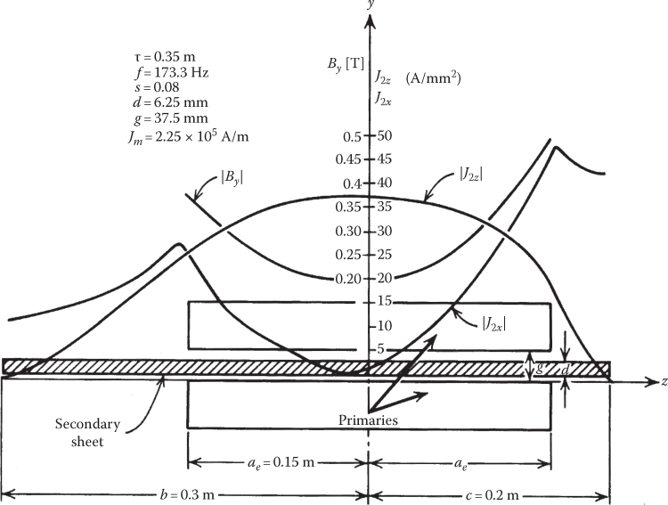
FIGURE 3.9 Airgap flux density and secondary current density components in the presence of edge effect (b ≠ c). (After Nasar, S.A. and Boldea, I., Linear Motion Electric Machines, John Wiley & Sons, New York, 1976.)

Doing this, Ref. [6] has found for b = c (symmetrically placed secondary), for the active power ratio, a reduction coefficient k_tr of equivalent conductivity σ_e of aluminum sheet:

σ e = σ ( k s k i n \times k t r ) (3.39)

$σ_{e} = \frac{σ}{(k_{s k i n} \times k_{t r})} (3.39)$

k t r = k 2 x k R \cdot [1 + S \cdot G 2 e t \cdot k 2 R / k 2 x 1 + S 2 \cdot G 2 e t] \geq 1 (3.40)

$k_{t r} = \frac{k_{x}^{2}}{k_{R}} \cdot [\frac{1 + S \cdot G_{e t}^{2} \cdot k_{R}^{2} / k_{x}^{2}}{1 + S^{2} \cdot G_{e t}^{2}}] \geq 1 (3.40)$

k t r = k 2 R k x \approx 1; k R = 1 - Re [(1 - S \cdot G e t) \cdot λ α \cdot a e \cdot tanh (α \cdot a e)] (3.41)

$k_{t r} = \frac{k_{R}^{2}}{k_{x}} \approx 1; k_{R} = 1 - Re [(1 - S \cdot G_{e t}) \cdot \frac{λ}{α \cdot a_{e}} \cdot \tanh (α \cdot a_{e})] (3.41)$

k x = 1 + Re [(S \cdot G e t + j) \cdot S \cdot G e t \cdot λ α \cdot a e \cdot tanh (α \cdot a e)] (3.42)

$k_{x} = 1 + Re [(S \cdot G_{e t} + j) \cdot \frac{S \cdot G_{e t} \cdot λ}{α \cdot a_{e}} \cdot \tanh (α \cdot a_{e})] (3.42)$

λ = 1 1 + 1 + j \cdot S \cdot G e t - - - - - - - - - - - \sqrt \cdot tan ( α \cdot a e ) \cdot tanh π τ \cdot ( c - a e ) (3.43)

$λ = \frac{1}{1 + \sqrt{1 + j \cdot S \cdot G_{e t}} \cdot \tan (α \cdot a_{e}) \cdot \tanh \frac{π}{τ} \cdot (c - a_{e})} (3.43)$

For low values of S • G_et(S • G_et < < 1) and (or) narrow primaries 2 • a_e/τ < 0.3, k_tr yields the expression

k t r = 1 1 - tanh ( π τ \cdot a e ) π τ \cdot a e / [ 1 + tanh ( π τ \cdot a e ) tanh π τ ( c - a e ) ] \geq 1 (3.44)

$k_{t r} = \frac{1}{1 - \frac{\tanh (\frac{π}{τ} \cdot a_{e})}{\frac{π}{τ} \cdot a_{e}} / [1 + \tanh (\frac{π}{τ} \cdot a_{e}) \tanh \frac{π}{τ} (c - a_{e})]} \geq 1 (3.44)$

The edge effect may be considered by simply reducing the equivalent electric conductivity of the secondary by k_tr; in general, k_tr is to be reduced to decrease the secondary Joule losses and increase the goodness factor, which now yields the formula

G e = G e t k t r = μ 0 \cdot τ 2 \cdot ω 1 \cdot σ A L \cdot d A L π \cdot k t r \cdot k s k i n \cdot ( g \cdot k c \cdot k F r ) (3.45)

$G_{e} = \frac{G_{e t}}{k_{t r}} = \frac{μ_{0} \cdot τ^{2} \cdot ω_{1} \cdot σ_{A L} \cdot d_{A L}}{π \cdot k_{t r} \cdot k_{s k i n} \cdot (g \cdot k_{c} \cdot k_{F r})} (3.45)$

Values of k_tr ≈ 1.3–1.5 lead to reasonable overhangs (c − a = τ/π) and thus limit secondary costs. As G_e lumps influences of skin effect, airgap fringing, stator slotting, and edge effect, it becomes the key variable in characterizing LIM performance, besides the number of poles 2p and slip S, frequency ω₁, and stator mmf (or J_1m).

But before switching to the study of dynamic end effect, let us generalize these results on edge effects to SLIMs as they are more practical, due to secondary ruggedness and reasonable track costs.

3.2.5 Edge Effects for SLIMs

A SLIM for short excursion (a few meters) may use a ladder-laminated core secondary to obtain high efficiency (above 0.8) and good power factor (above 0.7) for mechanical gaps of less than 1.5 mm. SLIMs do not experience edge effects and should be treated as rotary IMs unless the number of poles 2p = 2, 4, when the static end effect occurs, as already mentioned in this chapter. For excursions longer than a few meters, the cost of secondary becomes important and thus an aluminum sheet on secondary becomes important and, consequently, an aluminum sheet on iron secondary (Figure 3.10a) is the only economical solution. To increase the contribution of solid back iron of secondary to the thrust, the depth of penetration of the magnetic field in it should be increased, and making it of 3–4 pieces (“laminations”) seems the way to do it (Figure 3.10b).

To account for the edge effect in SLIMs with aluminum sheet on iron, we should first notice that

The secondary back-iron width is about equal to the “stack width” of primary, 2a, while the aluminum sheet (flat or bent toward back-iron sides for larger ruggedness) is wider, to produce enough thrust. Also, to counteract the lateral expulsion force on the aluminum sheet by a self-centering force due to the primary and secondary iron cores, in case of off-center (laterally) placement of the secondary with respect to primary, the secondary back-iron width equals the primary stack length.
The airgap flux per pole has to close through the back iron along (basically) the field penetration depth δ_iron (3.15); fortunately, the division of secondary back iron into 3–4 “laminations”—Figure 3.10b leads to a pronounced edge effect in iron, which reduces the iron equivalent electrical conductivity:

$σ i e = (σ i r o n k t r i) (3.46)$ $σ_{i e} = (\frac{σ_{i r o n}}{k_{t r i}}) (3.46)$

Images

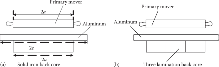
FIGURE 3.10 SLIM secondaries: (a) with solid back iron and (b) made of three “laminations.”

The k_tri coefficient for edge effect for i back-iron laminations may be considered based on Equation 3.40 with c = a_e and a_e/i instead of a_e:

k t r i \approx 1 1 - tanh ( π τ \cdot a e i ) π τ \cdot a e i (3.47)

$k_{t r i} \approx \frac{1}{1 - \frac{\tanh (\frac{π}{τ} \cdot \frac{a_{e}}{i})}{\frac{π}{τ} \cdot \frac{a_{e}}{i}}} (3.47)$

Now, the skin effect (3.15) in iron may be calculated with σ_ie and not with σ_iron.

Also, the back iron adds a “virtual length” to the airgap because it is very heavily saturated; the increased airgap g_e is

g s e \approx (1 + k s a t) \cdot (g + h A L) \cdot k c \cdot k F r (3.48)

$g_{s e} \approx (1 + k_{s a t}) \cdot (g + h_{A L}) \cdot k_{c} \cdot k_{F r} (3.48)$

The saturation coefficient k_sat in (3.43) stems from the reluctance ratio (of back iron and of airgap pole flux paths):

k s s \approx 2 τ 2 π 2 \cdot μ 0 2 \cdot ( g + h A L ) \cdot k c \cdot δ i \cdot μ i r o n (3.49)

$k_{s s} \approx \frac{{2τ}^{2}}{π^{2}} \cdot \frac{μ_{0}}{2 \cdot (g + h_{A L}) \cdot k_{c} \cdot δ_{i} \cdot μ_{i r o n}} (3.49)$

Let us note that δ_i (3.15) is dependent on μ_iron, which in turn depends on flux density B_ti tangential on the iron upper surface:

B t i \cdot δ i \approx B g \cdot τ π (3.50)

$B_{t i} \cdot δ_{i} \approx B_{g} \cdot \frac{τ}{π} (3.50)$

This is an alternative calculation of B_ti for given B_g1 (airgap flux density at rated (or peak) thrust) or B_ti ≈ 2 T (or in general, as required).

Now, again, we may lump up the iron contribution to thrust by an increase in the equivalent conductivity of secondary σ_se:

α s e = σ A L k t r A L \cdot k s k i n \cdot (1 + σ i σ A L \cdot δ i \cdot k t r A L \cdot k s k i n k t i \cdot d A L) = σ A L k t r A L \cdot k s k i n (1 + k i s) (3.51)

$α_{s e} = \frac{σ_{A L}}{k_{t r A L} \cdot k_{s k i n}} \cdot (1 + \frac{σ_{i}}{σ_{A L}} \cdot \frac{δ_{i} \cdot k_{t r A L} \cdot k_{s k i n}}{k_{t i} \cdot d_{A L}}) = \frac{σ_{A L}}{k_{t r A L} \cdot k_{s k i n}} (1 + k_{i s}) (3.51)$

In (3.51) the equivalent (active) thickness of back iron is δ_i and has to be calculated iteratively. The secondary back-iron contribution to thrust is lumped up in the aluminum sheet equivalent conductivity σ_se. An equivalent goodness factor G_se may be defined again with g_se and σ_se:

G s e = μ 0 \cdot τ 2 \cdot ω 1 π 2 \cdot d A L g s e \cdot σ s e (3.52)

$G_{s e} = \frac{μ_{0} \cdot τ^{2} \cdot ω_{1}}{π^{2}} \cdot \frac{d_{A L}}{g_{s e}} \cdot σ_{s e} (3.52)$

Note: It may be argued that the skin effect in the iron also shifts the phase of the current density along the iron depth and thus an additional leakage inductance (or “reactive” conductivity) is added.

3.3 Dynamic End-Effect Quasi-One-Dimensional Field Theory

Let us consider a 2p pole single-layer winding short-primary long-secondary DLIM whose primary is moving at speed U < U_s; U_s—the traveling primary mmf. Speed (U_s = 2+τ.f₁) (Figure 3.11). The phase shifting of eddy current in secondary iron may be considered through a leakage reactance equal to its resistance: S • ω₁ • L_2li = R′_2i • R′_2i is related to total secondary resistance as in (3.46) by the coefficient k_iσ. Also notice that the lateral force (Figure 3.8c) j_x × B_y by aluminum currents becomes decentralizing when the secondary is placed asymmetrically in the lateral direction (0y): For SLIM the solid back iron adds two lateral forces, one decentralizing (due to its eddy currents) and one centralizing (due to iron).

The contour c₀(t₀) of secondary is in time in positions c₁(t₁), c₂(t₂), c₃(t₃), c₄(t₄), with respect to the moving primary.

In position c₀, there is no magnetic flux and so no induced voltage or current occurs.

When we consider contour c₂, there is a strong variation of magnetic flux in it and thus additional currents occur along the contour (secondary). As the primary moves and contour c₂ position is reached, the current induced in position c₁ has already decreased by the secondary electrical time constant (calculated as for a rotary IM) T_e2:

T e 2 \approx L m ( g m ) R ' 2 = G e ω 1 (3.53)

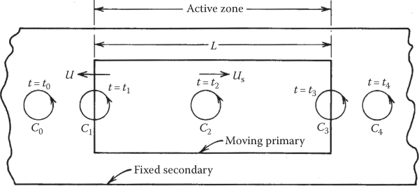
$T_{e 2} \approx \frac{L_{m} (g_{m})}{{R^{'}}_{2}} = \frac{G_{e}}{ω_{1}} (3.53)$

Images

FIGURE 3.11 Dynamic end effect. (After Nasar, S.A. and Boldea, I., Linear Motion Electric Machines, John Wiley & Sons, New York, 1976.)

where

L_m is the magnetization inductance (the secondary leakage inductance is almost zero for aluminum sheet secondary once the airgap fringing effect has been considered).

R′₂ is the secondary equivalent resistance reduced to the primary; the expressions of L_m and R′₂ are calculated as if the machine were rotary with 2p poles but identical geometry of primary and secondary.

It is a known fact that if the speed is high, U_rated > 20 m/s (100 m/s, for a 360 km/h in highspeed trains), the mechanical and the magnetic airgap g_m is large, but still the conventional performance (without dynamic end effect) increases with higher goodness factor (G_e)—as in rotary IMs. A G_e ≥ 20 at f₁ = 175 Hz (τ = 0.35 m, 2p = 10) should be typical for a high-speed application.

But in this case, 3T_e2 = (3 × 20)/(2 •π•175) = 0.055 s. For a slip S = 0.08, the LIM speed would be

U = 2 τ f 1 (1 - S) = 2 \cdot 0.35 \cdot 175 \cdot (1 - 0.08) = 112.7 m / s (3.54)

$U = 2 τ f_{1} (1 - S) = 2 \cdot 0.35 \cdot 175 \cdot (1 - 0.08) = 112.7 m / s (3.54)$

The length traveled during three time constants (3T_e2) would be L_lef = U × 3T_e2 = 112.7 × 0.055 = 6. 198 m; the length of the primary L = 2pτ = 10 × 0.35 = 3.5 m. Consequently, the additional (dynamic end-effect-produced) entry secondary currents would not die out before, but rather after, the LIM primary exit end. It means a notable dynamic end effect or a high-speed LIM. But in the position of exit-end c₃, new additional dynamic end-effect currents occur. However, these currents would die out with a different (much smaller) time constant introduced here as T_exit:

T e x i t = L m e x i t ( τ / π ) R ' 2 = G e x i t R ' 2; g m e x i t = τ / π (3.55)

$T_{e x i t} = \frac{L_{m e x i t} (τ / π)}{{R^{'}}_{2}} = \frac{G_{e x i t}}{{R^{'}}_{2}}; g_{m e x i t} = τ / π (3.55)$

The equivalent airgap behind the primary (Figure 3.11) corresponds to an average flux line length in air, which is approximately τ/π, because the current periodicity is still τ at initiation (there are two primaries in DLIMs); for a SLIM g_{m exit}= τ/π, still, as half the travel of flux lines is considered to take place in the back iron.

For the same example (with g_m = 37.5 mm), the new time constant is 3 • T_exit = 3 • T_e2 • (g_m • π)/τ = 0.055•37.5/(2•350)×π = 0.00925s; the corresponding exit field “tail” length would be L_exit ≈ 3T_exit•U = 0.0925 × 112.7 = 1.0425 m.

Now these additional secondary currents are due to the motion of a short primary in front of a long secondary, and thus the dynamic end effects manifest themselves as follows:

The existence of additional secondary current density components both within the active zone (decaying with the T_e2 time constant) and in the primary tail (x > 2pτ, decaying with T_exit < 3 •T_e2 in general).
Consequently, considering the primary core to be infinitely long would exaggerate grossly the exit dynamic end effect, though most 1–2 DLIM field theories rely on it [4,7–9]. It may be safe to say that this exit-end part of dynamic end effect (in the tail of LIM primary) produces only additional secondary losses (besides a small reluctance braking force [3]).

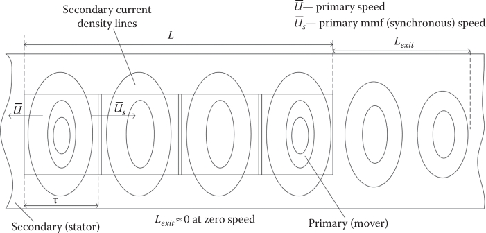
FIGURE 3.12 Secondary current density lines in a high-speed LIM (L_exit ≫ τ).
The dynamic end effect in the entry zone (x < 0) may be considered zero (Figure 3.11).
The dynamic end effect in active zone (0 ≤ x ≤ 2pτ) is the most important, and, as expected, it produces additional secondary current losses, demagnetization of the machine (a reduction of secondary power factor), and a dynamic end-effect force F_{x end}, which at zero slip may be propulsive (in lower goodness factor LIMs) or braking (for large dynamic end effect: high speed) (Figure 3.12).
Though there are two main types of primary windings, 2p pole single layer and 2p + 1 double layer (with half-filled end slots); they behave very similarly with respect to dynamic end effect. The two-step increase in primary mmf in the half-filled slots of entry end pole does not reduce the dynamic end effect if its attenuation length L_ef is larger than a pole pitch τ. It suffices to consider, in a first approximation, not 2p + 1 poles but approximately L = 2pτ if p > 4.
Only the fundamental of primary mmf θ₁(x, t) traveling wave is considered here (or its primary linear current sheet J₁(x, t)); also, all variables vary sinusoidally in time.
The other effects, typical to a sheet secondary and large airgap, are lumped into the equivalent goodness factor G_e.
Other more subtle consequences of dynamic end effect will surface on the way of unfolding the quasi 1D field theory of LIMs in the following sections. We will call this a technical theory as it is suitable for design and for defining the circuit model parameters (with dynamic end effect) in the next chapter.

Let us consider the DLIM with the increased airgap in the primary core extended to infinity (Figure 3.13) but at larger airgap (τ/π).

Because we are dealing with a sinusoidal time and space variation of primary current sheet J₁, complex variables may be used:

J ¯ ¯ 1 = J m \cdot e j \cdot (ω 1 \cdot t - π τ x) (3.56)

${\underline{J}}_{1} = J_{m} \cdot e^{j \cdot (ω_{1} \cdot t - \frac{π}{τ} x)} (3.56)$

Equation 3.56 is written in primary coordinates. We split the infinite-length model in three regions and apply Maxwell equations with a normal (single) airgap flux density component (along 0y) and a single variation, along the direction of motion x. The secondary current density has only one component J_z(x); the sinusoidal time variations are well understood.

The active zone (0 < x < 2pτ).

Images

FIGURE 3.13 LIM model for technical field theory.

Ampere’s law along contour a₁b₁c₁d₁ in Figure 3.13 leads to

g e \cdot \partial H \partial x = J m \cdot e j \cdot (ω 1 t - π τ x) + J 2 \cdot d A L (3.57)

$g_{e} \cdot \frac{\partial H}{\partial x} = J_{m} \cdot e^{j \cdot (ω_{1} t - \frac{π}{τ} x)} + J_{2} \cdot d_{A L} (3.57)$

From Faraday’s law,

\partial J 2 \partial x = j ω 1 \cdot μ 0 \cdot σ e \cdot d A L g e \cdot H y + μ 0 \cdot U \cdot σ e \cdot d A L g e \cdot \partial H y \partial x (3.58)

$\frac{\partial J_{2}}{\partial x} = j ω_{1} \cdot μ_{0} \cdot σ_{e} \cdot \frac{d_{A L}}{g_{e}} \cdot H_{y} + μ_{0} \cdot U \cdot σ_{e} \cdot \frac{d_{A L}}{g_{e}} \cdot \frac{\partial H_{y}}{\partial x} (3.58)$

where

U is the relative speed of primary with respect to secondary

H_y is the resultant magnetic field in the airgap

From (3.57) through (3.58) we obtain

\partial 2 H y \partial x 2 - μ 0 \cdot σ e \cdot d A L g e \cdot U \cdot \partial H y \partial x - j \cdot ω 1 \cdot μ 0 \cdot U \cdot σ e \cdot d A L g e = - j \cdot π τ \cdot g e \cdot J m \cdot e - j π τ x (3.59)

$\frac{\partial^{2} H_{y}}{\partial x^{2}} - μ_{0} \cdot σ_{e} \cdot \frac{d_{A L}}{g_{e}} \cdot U \cdot \frac{\partial H_{y}}{\partial x} - j \cdot ω_{1} \cdot μ_{0} \cdot U \cdot σ_{e} \cdot \frac{d_{A L}}{g_{e}} = - j \cdot \frac{π}{τ \cdot g_{e}} \cdot J_{m} \cdot e^{- j \frac{π}{τ} x} (3.59)$

The characteristic equation of (3.59) is

γ 2 - μ 0 \cdot σ e \cdot d A L g e \cdot U \cdot γ - j \cdot ω 1 \cdot μ 0 \cdot σ e \cdot d A L g e = 0 (3.60)

$γ^{2} - μ_{0} \cdot σ_{e} \cdot \frac{d_{A L}}{g_{e}} \cdot U \cdot γ - j \cdot ω_{1} \cdot μ_{0} \cdot σ_{e} \cdot \frac{d_{A L}}{g_{e}} = 0 (3.60)$

with the roots

γ ¯ 1, 2 = a 1 2 \cdot (\pm b 1 + 1 2 - - - - - - \sqrt + 1) \pm a 1 2 \cdot j \cdot b 1 - 1 2 - - - - - - \sqrt = γ 1, 2 r \pm j \cdot γ r (3.61)

${\underline{γ}}_{1, 2} = \frac{a_{1}}{2} \cdot (\pm \sqrt{\frac{b_{1} + 1}{2}} + 1) \pm \frac{a_{1}}{2} \cdot j \cdot \sqrt{\frac{b_{1} - 1}{2}} = γ_{1, 2 r} \pm j \cdot γ_{r} (3.61)$

where

a 1 = μ 0 \cdot σ e \cdot d A L g e \cdot U = π τ \cdot G e \cdot (1 - S) (3.62)

$a_{1} = μ_{0} \cdot σ_{e} \cdot \frac{d_{A L}}{g_{e}} \cdot U = \frac{π}{τ} \cdot G_{e} \cdot (1 - S) (3.62)$

b 1 = 1 + (4 G e \cdot ( 1 - S ) 2) 2 - - - - - - - - - - - - - - - - - -  ⎷   (3.63)

$b_{1} = \sqrt{1 + {(\frac{4}{G_{e} \cdot {(1 - S)}^{2}})}^{2}} (3.63)$

The complete solution of (3.60) is

H a = A \cdot e γ 1 \cdot x + B \cdot e γ 2 \cdot x + B m \cdot e - j \cdot π τ \cdot x (3.64)

$H_{a} = A \cdot e^{γ_{1} \cdot x} + B \cdot e^{γ_{2} \cdot x} + B_{m} \cdot e^{- j \cdot \frac{π}{τ} \cdot x} (3.64)$

B n = j \cdot τ \cdot J m π \cdot g e \cdot ( 1 + j \cdot S \cdot G e ) (3.65)

$B_{n} = j \cdot \frac{τ \cdot J_{m}}{π \cdot g_{e} \cdot (1 + j \cdot S \cdot G_{e})} (3.65)$

Entry zone (x ≤ 0) and exit zone (x ≥ 2pτ).

With no primary currents in these zones and an equivalent airgap g_exit = τ/π (G_exit ≪ G_e),

H e n t r y = C \cdot e γ 1 e x i t, for x \leq 0 (3.66)

$H_{e n t r y} = C \cdot e^{γ_{1 e x i t}}, for x \leq 0 (3.66)$

H e x i t = D \cdot e γ 2 e x i t \cdot (x - 2 \cdot p \cdot τ) for x \geq 2 p τ (3.67)

$H_{e x i t} = D \cdot e^{γ_{2 e x i t} \cdot (x - 2 \cdot p \cdot τ)} for x \geq 2 p τ (3.67)$

γ ¯ 1 e x i t = (γ ¯ 1) g e = τ π G e x i t; γ ¯ 2 e x i t = (γ ¯ 2) g e = τ π G e x i t (3.68)

${\underline{γ}}_{1 e x i t} = {({\underline{γ}}_{1})}_{\begin{array}{l} g_{e} = \frac{τ}{π} \\ G_{e x i t} \end{array}}; {\underline{γ}}_{2 e x i t} = {({\underline{γ}}_{2})}_{\begin{array}{l} g_{e} = \frac{τ}{π} \\ G_{e x i t} \end{array}} (3.68)$

The continuity conditions of magnetic field and current density at entry and exit ends (x = 0, 2pτ) yield

(H e n t r y) x = 0 = (H a) x = 0; (H e x i t) x = 2 p τ = (H a) x = 2 p τ (\partial H e n t r y \partial x) x = 0 = (J 2) x = 0; (\partial H e x i t \partial x) x = 2 p τ = (J 2) x = 2 p τ (3.69)

$\begin{array}{l} {(H_{e n t r y})}_{x = 0} = {(H_{a})}_{x = 0}; {(H_{e x i t})}_{x = 2 p τ} = {(H_{a})}_{x = 2 p τ} \\ {(\frac{\partial H_{e n t r y}}{\partial x})}_{x = 0} = {(J_{2})}_{x = 0}; {(\frac{\partial H_{e x i t}}{\partial x})}_{x = 2 p τ} = {(J_{2})}_{x = 2 p τ} \end{array} (3.69)$

We may replace the second boundary condition in (3.69) by

\int - \infty \infty H d x = 0 (3.70)

$\int_{- \infty}^{\infty} H d x = 0 (3.70)$

to get more realistic results.

However, using γ¯1 ${\underline{γ}}_{1}$ in the entry zone (not γ¯1 entry ${\underline{γ}}_{1 e n t r y}$ ) and γ₂ in the exit zone, as done in most literature (infinite core length), we get easily A, B, C, D constants as

A = - j \cdot J m Δ \cdot (γ 2 β + S \cdot G e) \cdot e - 2 p \cdot τ \cdot γ 1 B = j \cdot J m Δ \cdot (γ 1 β + S \cdot G e)

$\begin{matrix} A = - j \cdot \frac{J_{m}}{Δ} \cdot (\frac{γ_{2}}{β + S \cdot G_{e}}) \cdot e^{- 2 p \cdot τ \cdot γ_{1}} \\ B = j \cdot \frac{J_{m}}{Δ} \cdot (\frac{γ_{1}}{β + S \cdot G_{e}}) \end{matrix}$

Δ = g e \cdot (γ 2 - γ 1) \cdot (1 + j \cdot S \cdot G e) C = A \cdot (1 - e - 2 p \cdot τ \cdot γ 1) D = B \cdot (1 - e 2 p \cdot τ \cdot γ 2) (3.71)

$\begin{array}{l} Δ = g_{e} \cdot (γ_{2} - γ_{1}) \cdot (1 + j \cdot S \cdot G_{e}) \\ C = A \cdot (1 - e^{- 2 p \cdot τ \cdot γ_{1}}) \\ D = B \cdot (1 - e^{2 p \cdot τ \cdot γ_{2}}) \end{array} (3.71)$

To make a technical compromise, we may use the value of C and D from (3.71) into (3.66) through (3.67) and then calculate J_exit(x, t) (with J_entry ≈ 0) and the corresponding exit end secondary Joule losses at a more realistic value.

3.3.1 Dynamic End-Effect Waves

The airgap flux density in the airgap (active zone) B_ag (μ₀ • H_a in Equation 3.64) has a first conventional term (typical to rotary IMs: or for LIMs with “infinite length”) and two additional terms known as end-effect waves [1]: one forward wave µ₀ • A • e^2pτ−γ₁ ^x and one backward wave (μ0⋅B⋅eγ¯2⋅x) $(μ_{0} \cdot B \cdot e^{{\underline{γ}}_{2} \cdot x})$ :

B ¯ ¯ ¯ e n d - = μ 0 \cdot A \cdot e γ 1 \cdot x = - j \cdot μ 0 \cdot J 1 m Δ \cdot (γ 2 β + S \cdot G e) \cdot e (γ 1 r + j \cdot γ i) \cdot (x - 2 p τ) (3.72)

${\underline{B}}_{e n d -} = μ_{0} \cdot A \cdot e^{γ_{1} \cdot x} = - j \cdot μ_{0} \cdot \frac{J_{1 m}}{Δ} \cdot (\frac{γ_{2}}{β} + S \cdot G_{e}) \cdot e^{(γ_{1 r} + j \cdot γ_{i}) \cdot (x - 2 p τ)} (3.72)$

B ¯ ¯ ¯ e n d + = μ 0 \cdot B \cdot e γ ¯ 2 \cdot x (3.73)

${\underline{B}}_{e n d +} = μ_{0} \cdot B \cdot e^{\underline{γ} 2 \cdot x} (3.73)$

B ¯ ¯ ¯ e n d + = j \cdot μ 0 \cdot J 1 m Δ \cdot (γ 1 β + j \cdot S \cdot G e) \cdot e γ 2 r \cdot x \cdot e - j \cdot γ i \cdot x (3.74)

${\underline{B}}_{e n d +} = \frac{j \cdot μ_{0} \cdot J_{1 m}}{Δ} \cdot (\frac{γ_{1}}{β} + j \cdot S \cdot G_{e}) \cdot e^{γ_{2 r} \cdot x} \cdot e^{- j \cdot γ_{i} \cdot x} (3.74)$

They are also called entry end and exit end waves [1].

Both waves are characterized by the same pole pitch τ_e=1/γ_i, but they are attenuated along the direction of motion differently as |γ_1r| ≫ γ_2r (Equation 3.61). Typical values of 1/γ_1r • τ and 1/γ_2r • τ for a DLIM, as a function of goodness factor for two typical slip values (S = 0 and S = 0.08), are given in Figure 3.14 (based on Equation 3.61).

It is obvious that the entry end wave (Figure 3.14a) is penetrating a very short length (less than 10% of a pole pitch), and thus its effects may be neglected. In contrast, the exit-end wave penetration depth (Figure 3.14b) may be large and increases almost linearly with goodness factor.

For a DLIM, at 100 m/s and τ = 0.35 m and G_e ≈ 24–28, the exit end wave penetration depth would be about 6 pole pitches (2.1 m), not far away from the approximate prediction made earlier in this paragraph. For an urban LIM transport system U ≈ 30 m/s and τ = 0.25–0.3 m, still G_e ≈ 15–20 and thus the attenuation length of exit-end wave would be 4–5 pole pitches; consequently a LIM with 7–9 poles would experience a notable but perhaps still reasonable dynamic end effect.

Let us now explore the pole pitch of the exit-end wave τ_e/τ = 1/γ_i at S = 0 and 0.08 versus goodness factor (Figure 3.15, from (3.61)):

τ e τ \approx U s e U = 2 G e \cdot ⎛ ⎝ ⎜ 1 + 16 G 2 e \cdot ( 1 - S ) \sqrt - 1 2 ⎞ ⎠ ⎟ 1 / 2 (3.75)

$\frac{τ_{e}}{τ} \approx \frac{U_{s e}}{U} = \frac{2}{G_{e} \cdot {(\frac{\sqrt{1 + \frac{16}{G_{e}^{2} \cdot (1 - S)}} - 1}{2})}^{1 / 2}} (3.75)$

Images

FIGURE 3.14 Relative penetration depths of end-effect waves: (a) entry end wave and (b) exit end wave.

Images

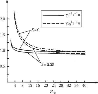
FIGURE 3.15 Relative pole pitch (τ_e/τ) of end-effect waves versus goodness factor for slip S = 0, 0.08. (After Nasar, S.A. and Boldea, I., Linear Motion Electromagnetic Devices, Taylor & Francis, New York, 2001.)

It is very evident that, at small values of goodness factor (when the dynamic end (dynamic) effect is smaller anyway), the speed of end-effect waves is larger than the synchronous speed; so, as expected, at S = 0, the end-effect force has a braking character, thus reducing the mechanical power produced by the high-speed LIM.

As the LIM length for a vehicle may not go over 2–4 m due to necessity to negotiate tight curves, it seems that with G_e = 10–25 for LIMs from 30 to 120 m/s, the dynamic end effect will always be present. To improve performance, efficiency means to reduce end effects, and (or) optimal design methods should be used, as both conventional and end effects increase with the goodness factor.

3.3.2 Dynamic End-Effect Consequences in a DLIM

The main consequences of dynamic end effect are

Reduction of thrust
Higher secondary Joule losses (lower efficiency)
Higher absorbed reactive power (lower power factor)
Nonuniform airgap flux density, thrust, normal force along DLIM length

The thrust is composed of two components (conventional F_xc and end-effect force F_xe):

F x c = μ 0 \cdot a \cdot J 1 \cdot Re ⎛ ⎝ ⎜ \int 0 2 p τ B * n d x ⎞ ⎠ ⎟ (3.76)

$F_{x c} = μ_{0} \cdot a \cdot J_{1} \cdot Re (\int_{0}^{2 p τ} B_{n}^{*} d x) (3.76)$

F x e = μ 0 \cdot a \cdot J 1 \cdot Re ⎛ ⎝ ⎜ \int 0 2 p τ B * \cdot e γ * 2 \cdot x \cdot e - j \cdot β \cdot x d x ⎞ ⎠ ⎟ (3.77)

$F_{x e} = μ_{0} \cdot a \cdot J_{1} \cdot Re (\int_{0}^{2 p τ} B^{*} \cdot e^{γ_{2}^{*} \cdot x} \cdot e^{- j \cdot β \cdot x} d x) (3.77)$

The ratio of the two force components f_e is

f e = F x e F x c = Re [ B * \cdot ( - 1 + exp 2 p \cdot τ \cdot ( y * 2 - j \cdot β ) y * 2 - j \cdot β ) ] Re ( B * n \cdot 2 p \cdot τ ) = (1 + S 2 \cdot G 2 e) \cdot Re ⎡ ⎣ ⎢ j \cdot ( γ 1 β + S \cdot G e ) \cdot ( exp ( 2 p \cdot π \cdot ( γ * 2 β - j ) ) - 1 ) S \cdot G e \cdot 1 β \cdot ( γ * 2 - γ * 1 ) \cdot ( 1 - j \cdot S \cdot G e ) \cdot 2 p \cdot π \cdot ( γ * 2 β - j ) ⎤ ⎦ ⎥ (3.78)

$\begin{array}{l} f_{e} = \frac{F_{x e}}{F_{x c}} = \frac{Re [B^{*} \cdot (\frac{- 1 + \exp 2 p \cdot τ \cdot (y_{2}^{*} - j \cdot β)}{y_{2}^{*} - j \cdot β})]}{Re (B_{n}^{*} \cdot 2 p \cdot τ)} \\ = (1 + S^{2} \cdot G_{e}^{2}) \cdot Re [\frac{j \cdot (\frac{γ_{1}}{β} + S \cdot G_{e}) \cdot (\exp (2 p \cdot π \cdot (\frac{γ_{2}^{*}}{β} - j)) - 1)}{S \cdot G_{e} \cdot \frac{1}{β} \cdot (γ_{2}^{*} - γ_{1}^{*}) \cdot (1 - j \cdot S \cdot G_{e}) \cdot 2 p \cdot π \cdot (\frac{γ_{2}^{*}}{β} - j)}] \end{array} (3.78)$

Equation 3.78 is fairly general in the sense that the relative influence of dynamic end effect is dependent only on the number of poles 2p, slip S, and on the equivalent goodness factor G_e (which includes slot opening, airgap fringing, skin and edge effects, by correction coefficients). If we add the primary stack length transversally 2a and the primary electric current sheet J_n as variables, we see that the DLIM thrust is dependent only on five variables and only one of them, G_e, depends on secondary frequency, magnetic saturation, and other geometrical data of DLIM.

The end-effect force at zero slip switches from propulsion to braking mode with increasing G_e and decreasing number of poles (Figure 3.16).

For 2p = 8 poles, and different goodness factors, the dynamic end effect at small slips (Figure 3.17) shows how severely the end-effect braking character increases with the goodness factor G_e (implicitly with speed).

At low goodness factor values, the dynamic end-effect force changes from braking to propulsion mode once at small slip values, while for high goodness factors (high speed in general), it oscillates from propulsion to braking mode a few times (at a few slip values). As shown in a later chapter on LIM design, it is very tempting to choose as optimum goodness factor G_e0 its values for which the dynamic end-effect force at zero slip is zero [10]. Reasonable performance, without dynamic end-effect compensation, may be obtained this way, even for speeds up to 120 m/s. As Equation 3.61 shows, the airgap flux density (μ₀ • H_a) amplitude varies along the DLIM primary length (Figure 3.18a):

Images

FIGURE 3.16 Normalized dynamic end-effect force versus goodness factor at zero slip. (After Nasar, S.A. and Boldea, I., Linear Motion Electric Machines, John Wiley & Sons, New York, 1976.)

B a = μ 0 \cdot B n \cdot e - j \cdot π τ \cdot x + μ 0 \cdot B \cdot e γ 2 \cdot x + μ 0 \cdot A \cdot e γ 1 \cdot x (3.79)

$B_{a} = μ_{0} \cdot B_{n} \cdot e^{- j \cdot \frac{π}{τ} \cdot x} + μ_{0} \cdot B \cdot e^{γ_{2} \cdot x} + μ_{0} \cdot A \cdot e^{γ_{1} \cdot x} (3.79)$

Similarly, the secondary current density J₂ amplitude will vary along primary length:

J 2 = g e d A L \cdot [γ 1 \cdot A \cdot e γ 1 \cdot x + γ 2 \cdot B \cdot e γ 2 \cdot x - j \cdot S \cdot G e \cdot e - j \cdot β \cdot x \cdot J 1 g e \cdot ( 1 + j \cdot S \cdot G e )] (3.80)

$J_{2} = \frac{g_{e}}{d_{A L}} \cdot [γ_{1} \cdot A \cdot e^{γ_{1} \cdot x} + γ_{2} \cdot B \cdot e^{γ_{2} \cdot x} - \frac{j \cdot S \cdot G_{e} \cdot e^{- j \cdot β \cdot x} \cdot J_{1}}{g_{e} \cdot (1 + j \cdot S \cdot G_{e})}] (3.80)$

Consequently, the thrust will vary along primary length due to dynamic end effect:

F x = a \cdot Re ⎡ ⎣ ⎢ \int 0 2 p τ (J 2 \cdot B * a) d x ⎤ ⎦ ⎥ (3.81)

$F_{x} = a \cdot Re [\int_{0}^{2 p τ} (J_{2} \cdot B_{a}^{*}) d x] (3.81)$

This is illustrated in Figure 3.18b for an unusually large pole pitch τ (τ = 1 m, but for 2p = 6) and a reasonably low goodness factor G_e = 15.

Images

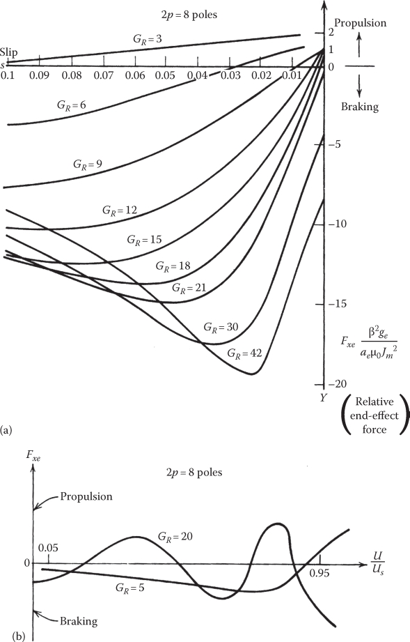
FIGURE 3.17 Normalized dynamic end-effect force versus slip for 2p = 8 poles and a few values of equivalent goodness factor values, (a), and the same force versus speed for low (G_e = 5) and high (G_e = 20 goodness factor and 2p = 8 poles), (b). (After Nasar, S.A. and Boldea, I., Linear Motion Electric Machines, John Wiley & Sons, New York, 1976.)

With an increased airgap in the primary tail, the decrease in the flux density after the end of primary core is much faster, as expected. We may now calculate the secondary power losses p₂ and the reactive power (Q₂):

p 2 = a \cdot d 2 σ e \cdot g e \cdot \int 0 2 p τ + L e x i t (J 2 \cdot J * 2) d x (3.82)

$p_{2} = \frac{a \cdot d^{2}}{σ_{e} \cdot g_{e}} \cdot \int_{0}^{2 p τ + L_{e x i t}} (J_{2} \cdot J_{2}^{*}) d x (3.82)$

Images

FIGURE 3.18 Airgap flux density and thrust density along the primary length. (After Nasar, S.A. and Boldea, I., Linear Motion Electric Machines, John Wiley & Sons, New York, 1976.)

The secondary losses in the “tail” of primary (x > 2p • τ) are considered here, as introduced earlier in this paragraph:

Q 2 \approx a \cdot ω 1 \cdot μ 0 \cdot g e \cdot \int 0 2 p τ (H a \cdot H * a) d x (3.83)

$Q_{2} \approx a \cdot ω_{1} \cdot μ_{0} \cdot g_{e} \cdot \int_{0}^{2 p τ} (H_{a} \cdot H_{a}^{*}) d x (3.83)$

We may define a secondary (or airgap) efficiency η₂ and power factor cos φ₂ to emphasize the dynamic end effects on them; the primary losses are added to yield the total efficiency:

η 2 = F x \cdot U F x \cdot U + p 2; cos φ 2 = F x \cdot U + p 2 ( F x \cdot U + p 2 ) 2 + Q 2 2 - - - - - - - - - - - - - - - \sqrt (3.84)

$η_{2} = \frac{F_{x} \cdot U}{F_{x} \cdot U + p_{2}}; \cos φ_{2} = \frac{F_{x} \cdot U + p_{2}}{\sqrt{{(F_{x} \cdot U + p_{2})}^{2} + Q_{2}^{2}}} (3.84)$

In the absence of dynamic end effect, η_2i = 1 − S.

A typical example of η₂ and cos φ₂ results for a high-speed LIM (U_s ≈ 120 m/s) with 2p = 12 and G_e = 31 shows acceptably good performance (Figure 3.19).

Images

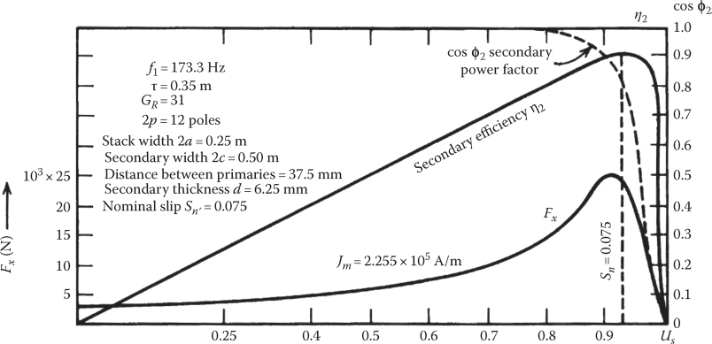
FIGURE 3.19 Secondary efficiency and power factor versus speed (p.u.) for a high-speed LIM (U_s ≈ 120 m/s).

In addition, the dynamic end effect leads to a gradual increase in core flux density along primary length. Also, the nonuniformity of the secondary current density produces two nonuniformly distributed normal forces: an attraction force F_na

F n a \approx μ 0 \cdot a \cdot \int 0 2 p τ | H a | 2 d x (3.85)

$F_{n a} \approx μ_{0} \cdot a \cdot \int_{0}^{2 p τ} {| H_{a} |}^{2} d x (3.85)$

and a repulsive one between one primary and the secondary

F n r 1 \approx μ 0 \cdot a \cdot d \cdot Re ⎡ ⎣ ⎢ \int 0 2 p τ \int 0 2 p τ J m 2 \cdot e - j β \cdot x 1 \cdot J 2 (x) d x d x 1 \cdot Δ 1 Δ 2 1 + ( x - x 1 ) 2 ⎤ ⎦ ⎥ (3.86)

$F_{n r_{1}} \approx μ_{0} \cdot a \cdot d \cdot Re [\int_{0}^{2 p τ} \int_{0}^{2 p τ} \frac{J_{m}}{2} \cdot e^{- j β \cdot x_{1}} \cdot J_{2} (x) d x d x_{1} \cdot \frac{Δ_{1}}{Δ_{1}^{2} + {(x - x_{1})}^{2}}] (3.86)$

Δ₁, Δ₂ = g₁, g₂—the distances between the aluminum plate and the two primaries of a DLIM.

For the second primary,

F n r 2 \approx F n r 1 Δ 2 Δ 1 (3.87)

$F_{n r 2} \approx F_{n r 1} \frac{Δ_{2}}{Δ_{1}} (3.87)$

After some approximations,

F n r 1 \approx 2 p \cdot τ Δ \cdot π \cdot μ 0 \cdot a \cdot J m 2 \cdot Re {γ * 2 \cdot B * \cdot [ exp ( γ * 2 - j \cdot β ) \cdot 2 p \cdot τ - 1 ] γ * 2 - j \cdot β + j \cdot S \cdot G e \cdot J m \cdot 2 p \cdot τ g e \cdot ( 1 - j \cdot S \cdot G e )} (3.88)

$F_{n r_{1}} \approx \frac{2 p \cdot τ}{Δ \cdot π} \cdot μ_{0} \cdot a \cdot \frac{J_{m}}{2} \cdot Re {\frac{γ_{2}^{*} \cdot B^{*} \cdot [\exp (γ_{2}^{*} - j \cdot β) \cdot 2 p \cdot τ - 1]}{γ_{2}^{*} - j \cdot β} + \frac{j \cdot S \cdot G_{e} \cdot J_{m} \cdot 2 p \cdot τ}{g_{e} \cdot (1 - j \cdot S \cdot G_{e})}} (3.88)$

In a DLIM, the repulsive normal force acts as a spring trying to keep the secondary in the middle of the airgap (Δ₂ = Δ₁); it also has a small damping effect on this “normal” motion.

Now adding the attraction and repulsive force F_na and F_nr, we may get in a high-speed DLIM, a resultant repulsive force in the first half of primary with an attraction total force in the second part of primary length (the so-called “dolphin” effect [7]).

In a SLIM, this latter effect also exists, and in Equation 3.80 we have to use twice J_m (total primary current sheet) and g_e in place of Δ.

If used for MAGLEVs, the SLIM normal forces, altered by the dynamic end effect, have to be considered in detail.

3.3.3 Dynamic End Effect in SLIMs

The technical theory of dynamic end effect applies in a similar way to SLIMs as it was developed in terms of equivalent airgap (g_e) and goodness factor G_e, with the amendment that the latter depends heavily on speed and primary mmf (on magnetic saturation, in fact). The contribution of solid back iron of secondary (made of 1, 2, 3 “solid” laminations) is to be considered by the inclusion of skin and edge effects as marked by magnetic saturation. Only some final results [11] are given here for a high-speed SLIM with f_n = 210 Hz, τ = 0.25 m, 2p + 1 = 13 poles (half-filled end slots), primary stack width 2a = 0.24 m, d_AL = 4 mm, mechanical gap g = 12 mm, σ_AL = 2.16 × 10⁷ Ω⁻¹m⁻¹, σ_i = 3.52 × 10⁶ Ω⁻¹m⁻¹ turns per phase: W₁ = 72, y/τ = 10/12 (chorded coils), primary current sheet amplitude J₁ = 1.5 × 10⁵ A turns/m.

Figure 3.20 shows the equivalent airgap and electric conductivity ratio for the three cases illustrating the influence of skin and edge effects and of secondary iron as additional conductive plate, versus slip; Figure 3.20b shows the secondary back-iron contribution to airgap increase (due to its magnetic reluctance).

The secondary back-iron penetration depth δ_i, the tangential flux density on its upper surface, and the equivalent goodness factor G_e versus slip at 400 A phase current J₁ = 1.55 × 10⁵ A turns/m are shown in Figure 3.21.

Finally, the thrust and normal forces (F_x, F_n) versus slip are illustrated in Figure 3.22a and the secondary efficiency and power factor in Figure 3.22b.

Airgap flux density, secondary current density, and the variation along primary length as influenced by dynamic end effect are similar to those presented for DLIM [11].

The SLIM and DLIM numerical examples related to dynamic end-effect technical (1D) field theory revealed results, which can be summarized as follows:

A quasi 1D theory of DLIM (and SLIM) may be developed simultaneously if the concept of equivalent airgap g_e and equivalent goodness factor G_e are used to lump the slot opening, airgap fringing, and skin and edge effects.
The 2p • τ primary winding type of DLIM is not crucial in influencing the dynamic end-effect consequences of airgap flux, secondary current density, and force density distribution along primary length.

Images

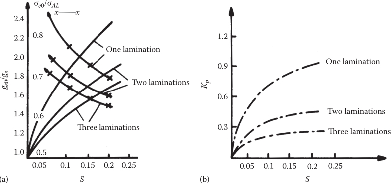
FIGURE 3.20 Equivalent airgap conductivity, (a), and p.u. secondary back-iron reluctance K_p versus slip for a high-speed SLIM with 1, 2, 3 “solid” lamination secondary back iron, (b). (After Nasar, S.A. and Boldea, I., Linear Motion Electromagnetic Devices, Taylor & Francis, New York, 2001.)

Images

FIGURE 3.21 Secondary back-iron penetration depth (δ_i) and surface-tangential flux density (B_xi), (a); equivalent goodness factor G_e versus slip (at 210 Hz and J₁ = 1.55 × 10⁵ A turns/m), (b). (After Nasar, S.A. and Boldea, I., Linear Motion Electromagnetic Devices, Taylor & Francis, New York, 2001.)

Images

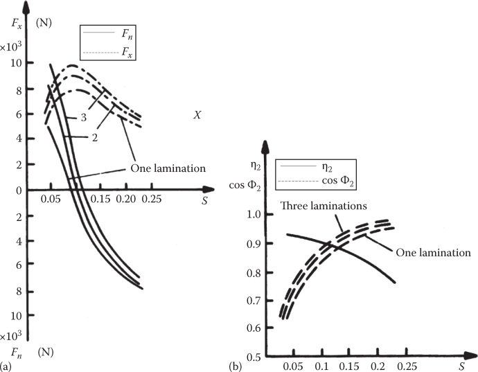
FIGURE 3.22 Secondary efficiency and power factor, (a); forces F_x, F_n versus slip for a high-speed SLIM, (b). (After Nasar, S.A. and Boldea, I., Linear Motion Electromagnetic Devices, Taylor & Francis, New York, 2001.)

The dynamic end-effect force, produced by the forward (exit-end) or end-effect wave, is motoring at low G_e (low-speed) LIMs and braking in character at high G_e (high speed) at zero slip, indicating the great divide between low-speed and high-speed LIMs.
As the technical theory uses only five variables to characterize LIMs, with given slip S and geometry (G_e, g_e, 2a (stack width) and primary electric current sheet J_m), it is fairly general and may be used in preliminary and optimal designs, as demonstrated indirectly in latter studies on LIMs for urban and interurban applications [12].

3.4 Summary of Analytical Field Theories of LIMs

As discussed in previous paragraphs, a complete analytical field theory of LIMs should account simultaneously for airgap slotting, airgap fringing, and skin and edge effect for the finite length of primary mmf distribution and of core length along the direction of motion.

Theoretically, such a theory was developed by using double Fourier decomposition of primary mmf along longitudinal (x) and transverse (z) directions and by variables separation; the magnetic field variation along airgap depth (y) may be thus calculated. To account for magnetic saturation and skin effect, the secondary for SLIM is decomposed into numerous layers of equivalent (but iteratively calculated) unique magnetic permeability. Also, the secondary back-iron length should be equal to aluminum sheet length to simplify the Fourier analysis along transverse direction, though it is feasible by proper boundary conditions to handle any back-iron width and also a secondary placed asymmetrically with respect to primary in the transverse direction.

For details see Ref. [13] (for DLIM) and [14, 15] (for SLIMs).

The Fourier series [16, 17] methods have been proposed for single-dimensional theories in third-order models [7] to deal with longitudinal end effect in DLIMs and SLIMs (with Al sheet on iron secondary [17] and with ladder winding [18, 19]).

On the other hand, Ref. [20] introduced a pole by pole unidimensional theory of dynamic end effect in DLIMs with remarkable insight into phenomena. However, for Fourier transform methods, the difficulty in calculating the self and mutual inductances and resistances of various fictitious secondary circuits (even in the absence of magnetic saturation) makes the method not easy to apply. Measuring these secondary–secondary and secondary–primary loops inductances by search coils may be a more practical way to get the circuit parameters required for the pole-by-pole method.

More recently, the wavelet analysis of LIM dynamic end effect was proposed [20] but apparently with no strong conclusion, yet, in terms of its practicality for LIM design or control.

Dynamic end effect in short-secondary (mover) and long-primary LIMs has also been studied [4,7,21] by analytical field theories but their applications are scarce. Wound-secondary doubly fed LIMs have also been investigated for short excursion (a few meters) transport applications, but their more practical theories are of circuit type and will be investigated in Chapter 4.

3.5 Finite Element Field Analysis of LIMs

The 3D nature of magnetic field distribution in LIMs with aluminum sheet on iron secondary, which experiences (in general) 2D current density trajectories, seems to suggest that the way to go is 3D-FEM. True, but from the start we need to mention that a complete analysis with thrust, normal force decentralizing lateral force, losses, efficiency, power factor, etc., versus speed characteristics would need, even today, tens of hours of computer time (Table 3.1, [22]), while the 3D analytical multiple-layer theory [14] would take a few minutes.

2D-FEM studies, one accounting for transverse (along 0z) and one accounting for slot opening, airgap fringing, and skin effect (along 0y), may be used to check (or duplicate) analytical results of equivalent airgap g_e and secondary conductivities σ_e, σ_i with which a second 2D-FEM (in x,y plane) would include magnetic saturation in the primary and secondary back iron and the dynamic end effect. Such a study may reduce to hours (from tens of hours for 3D-FEM) the total computation time of main LIM curves discussed earlier.

To illustrate the FEM, as applied to LIMs in terms of computation effort, a dual flat 2p = 4 poles primary SLIM with aluminum sheet-on-iron secondary was investigated by 3D-FEM (Figure 3.23) [22]:

The computation time is very large and thus, its use is, still, advisable only for special cases (situations).

TABLE 3.1
Discretization Data and CPU Time

Images

FIGURE 3.23 3D-FE mesh of LIM, (a); secondary eddy current density vectors, (b); thrust, (c); discretization data and computation time. (After Yamaguchi, T. et al., 3D FE analysis of a LIM with two armatures, Record of LDIA-2001, Nagano, Japan, pp. 300–303, 2001.)

A 2D-FEM investigation of a cage-secondary LIM is illustrated in Figure 3.24 [23].

As the amplitude of secondary depends on the contact resistance between the secondary bars and the sidebar (R_c), the normal force increases, the flux density distribution is perturbed, and the thrust decreases. The computation time is reasonable, and thus the 2D-FEM coupled circuit approach may be used extensively in LIM analysis.

3.6 Dynamic End-Effect Compensation

Though the dynamic end effect leads to a notable reduction of efficiency and power factor, the reduction of thrust in LIMs for transportation (urban at 20–30 m/s and interurban at up to 100–120 m/s) is a strong enough indicator expressing the ratio of end-effect thrust F_xe to conventional thrust (F_xe/F_xc(3.78)).

Images

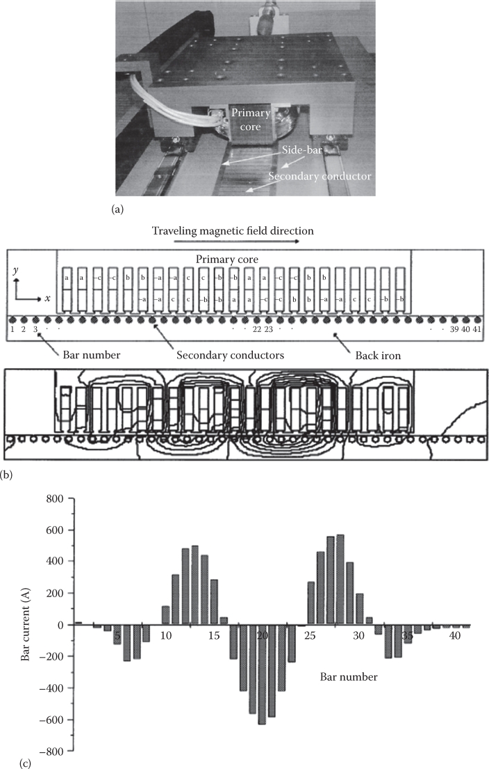
FIGURE 3.24 2D-FEM analysis of ladder cage-secondary SLIM: the lab model, (a), 2D model, (b), flux lines, (c), bar currents (R_c/R_e = 0.5; R_c, R_e—contact and side-bar segment resistances). (After Poloujadoff, M. and El Khashab, H., Eigen values and eigen functions: A tool to synthesize different models of LIMs, Record of LDIA-2001, Nagano, Japan, pp. 78–83, 2001.)

For the 30–120 m/s, at S = 0.1 the ratio F_xe/F_xc—dependent on G_e, 2p, S—varies in general in well-designed SLIMs in the interval of 0.2–0.6. This means a significant reduction of performance for high speed.

3.6.1 Designing at Optimum Goodness Factor

As both dynamic end effects and conventional performance grow with speed (with G_e increasing, for given 2p and S), it seems reasonable to assume that there is an optimum goodness factor G_e0. The criterion to calculate it depends on the objective function (max. thrust/primary weight, max thrust/Joule losses, max thrust per kVA at rated speed, etc.).

To simplify the problem and strike a compromise between criteria as mentioned previously, we use here the condition of zero end-effect force F_xe at S = 0 [10]:

(F x e) S = 0 = 0 \Rightarrow G e (2 p) (3.89)

${(F_{x e})}_{S = 0} = 0 \Rightarrow G_{e} (2 p) (3.89)$

Solving Equation 3.78 iteratively, we get G_e(2p), illustrated in Figure 3.25.

As expected, the optimum goodness factor G_e0, which includes quite a few parameters such as pole pitch (τ), primary frequency (ω₁), secondary equivalent conductivity (including skin effect and edge effect), and equivalent airgap (which includes slot opening, airgap fringing, secondary back-iron magnetic saturation), increases with the number of poles.

In general, designing at equivalent optimum goodness factor may reduce the end effect influence on total thrust at rated slip to 10%–15% at 30 m/s and 20%–25% at 120 m/s, under the condition that the maximum primary length is about 2.5 m for urban transportation and about 3.5 m for interurban vehicles, to facilitate negotiating tight curves. With pole pitches of 0.25–0.35 m, such conditions can be met.

3.6.2 LIMs in Row and Connected in Series

If further improvements are needed, a few SLIMs may be placed in row at a distance L_exit between each other (Figure 3.26a) [24].

Images

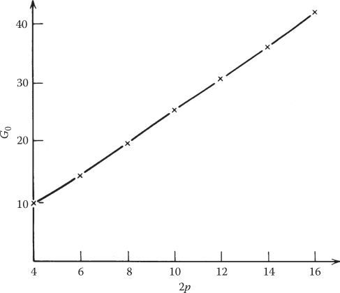
FIGURE 3.25 Optimum equivalent goodness factor G_e versus number of poles ((F_xe)_S=0 = 0).

Images

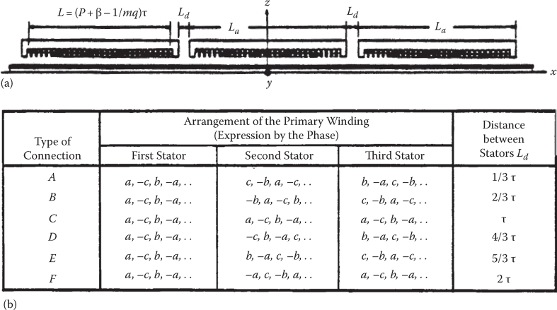
FIGURE 3.26 Series connection of SLIMs (a) 3 LIMs in series, (b) border of phases in 3 SLIMs in series.

The distance L_exit between the SLIMs in row is such that, at rated speed (slip), the exit end-effect magnetic flux density of first SLIM reaches the entry end of the next LIM at such an amplitude and phase that it reduces drastically the end-effect airgap flux density in the second SLIM. With L_exit= (1, 2, 3, 4, 5, 6) τ/3 and a certain sequence of phases (as in Figure 3.26b), such conditions can be met.

As illustrated in Ref. [24], the influence of dynamic end effect on thrust is thus reduced to, perhaps, 10% at 300 km/h for 3 SLIMs in row, 8 poles each, pole pitch τ = 0.3 m.

Besides these solutions, already in Refs. [1, 3], compensation windings in front of LIM have been proposed to reduce the dynamic end effects. But though the thrust has been increased, with slightly lower efficiency, there is apparently no progress in terms of total thrust/weight, which is essential in transportation.

3.6.3 PM Wheel for End-Effect Compensation

Quite a different dynamic end-effect compensation based on a PM wheel rotating at a speed slightly higher than SLIM speed and a pole pitch close to SLIM pole pitch has been proposed [25]—Figure 3.27.

At a certain core radius of PM wheel compensator (r_c = 75 mm [25]), the torque (Figure 3.27d) would be zero. In such conditions, the improvement in thrust (Figure 3.27b), in power factor (Figure 3.27c), and in efficiency (Figure 3.27c) is evident and effective.

But the cost of the PM wheels and their drive (one for each SLIM on a vehicle) is not trivial (the PMs are very thick), and it is not yet proven whether using the optimum goodness factor design and placing of SLIMs in row is not less costly for equivalent performance. So the jury is still out on this issue of dynamic end-effect compensation (reduction).

3.7 Summary

LIMs are counterparts of rotary IMs.
To reduce the cost of the long secondary extended over the entire excursion length, the latter is made of an aluminum sheet on solid back iron (for SLIMs) or solely an aluminum sheet in DLIMs.

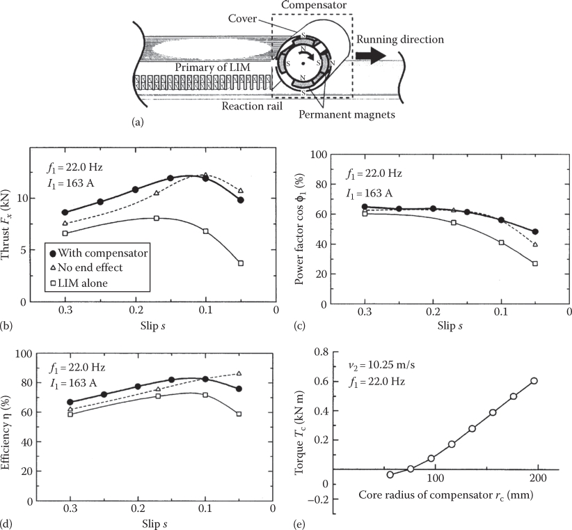
FIGURE 3.27 PM wheel for dynamic end-effect compensation; (a) the topology (2p = 8, τ = 0.28 m, f₁ = 22 Hz, S_n = 0.17, v = 10 m/s); (b) thrust; (c) power factor; (d) efficiency; (e) torque of the PM wheel. (After Fuji, N. et al., End effect compensator based on new concept for LIM, Record of LDIA-2001, Nagano, Japan, pp. 102–106, 2001.)
The SLIM is favored since the secondary is more rugged and less costly in general.
Besides the thrust, the LIM also produces normal force, which in a SLIM is repulsive at high secondary (slip) frequency S*f₁ and attraction in character for small slip frequency S*f₁ values.
In SLIMs with ladder (cage) secondary, placed in a laminated (or even solid) core, however, the resultant normal force is of attraction character and, at B_g = 0.6 T in the airgap, it may produce a normal force F_n ≥ 6F_xn (thrust) and thus “cover” a good part of vehicle weight; a few additional controlled electromagnets would provide the rest of the normal force for a MAGLEV operation.
Single-layer 2p (even) pole-count or double-layer 2p + 1 (odd) pole-count three-phase windings are the most practical solutions for flat LIMs. Tubular LIM will be discussed in a later chapter dedicated to low-speed, low-excursion length (less than 2 m) applications.
Simplified three-phase windings may be used in some applications; among them typical 12 slot/10 pole modules (or other combinations) are good candidates for low-thrust, low-speed, low-excursion length (copper losses are reduced) applications.
Due to the open character of LIM magnetic circuit along 0x (direction of motion) in the presence of Gauss flux law, the back-iron flux (in primary and secondary) is not 50% of airgap pole flux, as in rotary IMs, but it has points, one pole pitch apart, where full airgap flux is reached; this is in fact so for 2p < 10; to avoid heavy saturation of back iron, the later has to be designed with adequate depth (and limited pole pitch).
In LIMs with 2p < 6 (2p + 1 < 7), the self and mutual inductances between the three phases of primary are different from each other, and thus the phase currents are not symmetric; this is called the static end effect and should be accounted for in LIM control, to avoid thrust pulsations.
Skin effect is present in the LIM secondary (at frequency f₂ = S*f₁); a decrease in aluminum equivalent conductivity due to skin effect by a coefficient K_{R skin} > 1 is used for a practical design.
Skin effect is also manifest in the secondary solid back iron of SLIM, but here the magnetic saturation makes it more difficult to ascertain; for a given airgap flux density, tangential flux density Bt_max and the depth of field penetration δ_iron may be found iteratively, based on the B(H) curve of mild solid iron.
As the ratio of magnetic airgap g_m= g_air+ g_AL to pole pitch τ may reach 0.1, there is notable flux fringing (by 2D field distribution in the airgap “in the absence” of secondary conductivity) in the airgap, and a correction coefficient k_Fg > 1 increases g_m to account approximately for this phenomenon.
Though the magnetic airgap g_m (or g_m/2 in DLIMs) is rather large, the stator slot opening may be large enough (open slots for preformed primary coils) to produce a few percent of airgap pole flux reduction, and the Carter coefficient K_c > 1 (in a recent formulation) may be used to account for it (g_e= K_cg_m).
So the slot opening and airgap fringing lead to an increased equivalent airgap g_e = k_ck_Fgg_m.
Similarly, the equivalent secondary conductivity is decreased by skin effect σ_Alc = σ_AL/K_skin.
With g_e and σ_Alc, the transverse edge effect is approached; the transverse edge effect reflects the existence of two components J_z, J_x of secondary current density in the active zone (under LIM primary). The consequence is a nonuniform distribution of normal flux density along the transverse direction and additional Joule losses in secondary. In essence, two correction coefficients may account for this effect: the further reduction of secondary conductivity σ_e= σ_eA/k_TR and an increase in the airgap g_et= g_e/k_x (k_x ≤ 1, k_TR > 1).

For SLIMs, the equivalent airgap will further increase due to magnetic saturation: g_ete= g_et (1 + k_s), and the equivalent aluminum conductivity will increase to σ_se (3.46), to account for secondary solid iron conductivity and magnetic reluctance, approximately. When the secondary is placed asymmetrically (in the transverse direction), a decentralizing lateral force occurs due to transverse edge effect.
With the equivalent airgap and secondary conductivity, the dynamic end effect may be approached in a 1D field (technical) theory.
The dynamic end effect occurs as new secondary sections enter the airgap magnetic field zones. Thus, additional secondary currents are induced at LIM primary entry.
These additional secondary currents “born” at entry end decay toward the LIM primary end with the secondary electric time constant T_e ≈ G_e/ω₁, G_e = µ₀ (τ²ω₁/π²) (σ_ted_AL/g_te).
G_e is the goodness factor or the Reynolds magnetic number; it may be shown that G_e is equal to X_m/R′₂ with X_m—magnetization reaction, R′₂—secondary resistance.
It has been demonstrated that the influence of dynamic end effect depends essentially on G_e, S, 2p, 2a (stack width). G_e is a key variable, whose influence on performance is very strong.
The influence of dynamic end effect on airgap flux distribution (which becomes more and more nonuniform as the speed (or G_e) increases, for low slip values and a_e given and for given number of poles of primary). The end effect is basically portrayed by the so-called exit-end forward wave B_exit, which decays slowly (with T_e time constant), along primary length.
The pole pitch of B_exit, τ_e at S = 0 is larger than the primary mmf wave pole pitch τ for low values of G_e, and thus the end-effect thrust is motoring: for larger G_e, τ_e ≤ τ and thus the end-effect thrust is braking.
So, in high-speed LIMs (with high dynamic end effect), the end-effect thrust at S = 0 (or for S < 0.1) is braking.
Additionally, the dynamic end effect produces a reduction in power factor, efficiency, and thrust (power) in large speed (large G_e) LIMs.
To reduce the dynamic end effect, an optimal goodness factor G_e would be a reasonable compromise because both longitudinal end-effect intensity and conventional performance increase with G_e.
A G_e defined simply as corresponding to zero end-effect force at S = 0 seems a reasonable compromise [10]. G_e depends solely on 2p (pole counts) and increases rather linearly with 2p (G_e = 10 for 2p = 4 and G_e = 30 for 2p = 10).
Placing 2–3 LIMs in row at a precalculated distance (in between) and connected in series may produce further reduction in dynamic end effects.
Compensation windings have been proposed at the entry end of LIM [25, 26] to reduce the dynamic end effect in the main LIM; still no such solutions have been applied as they are not clearly superior in global performance/cost terms.
A PM wheel speeding above LIM speed and placed in front of LIM primary [27] was shown to produce better overall performance at zero torque of the wheel; still, the additional cost of the PM wheel makes the solution application at best a future goal.
As the LIM field analysis [28], a must for design, has been approached in this chapter, the circuit model, needed for dynamics and control, is the aim of the next chapter.

References

1. S. Yamamura, Theory of Linear Induction Motors, John Wiley & Sons, New York, 1972.

2. I. Boldea and L. Tutelea, Electric Machines, CRC Press, Taylor & Francis, New York, 2009.

3. S.A. Nasar and I. Boldea, Linear Motion Electric Machines, John Wiley & Sons, New York, 1976, Chapter 1.

4. S.A. Nasar and I. Boldea, Linear Motion Electromagnetic Devices, Taylor & Francis, New York, 2001, Chapter 3.

5. E. Matagne, Slot effect on the airgap reluctance Carter-like calculation suitable for electric machines with large air-gap or surface mounted permanent magnet, Electromotion, 15(4), 2008, 171–176.

6. H. Bolton, Transverse edge effect in sheet rotor induction machines, Proc. IEE, 116, 1969, 725–739.

7. E.R. Laithwaite, Induction Machines for Special Purposes, G. Newness, London, U.K., 1966.

8. M. Poloujadoff, The Theory of Linear Induction Motors, Clarendon Press, Oxford, U.K., 1980.

9. J.F. Gieras, Linear Induction Drives, Oxford University Press, Oxford, U.K., 1992.

10. I. Boldea and S.A. Nasar, Optimum goodness criterion for linear induction motor design, Proc. IEE, 123(1), 1976, 89–92.

11. I. Boldea and S.A. Nasar, Improved performance of high speed single-sided LIMs: A theoretical study; EMELDG International Quarterly (now EPCS Taylor & Francis), 2(2), 1978, 155–166.

12. I. Boldea and S.A. Nasar, Optical design criterion for linear induction motors, Proc. IEEE, 123(1), 1976, 89–92.

13. K. Oberretl, Three dimensional analysis of the linear motor taking into account edge effects and winding distribution, Arch. Electrotech., 55, 1973, 181–190.

14. I. Boldea and M. Babescu, Multilayer approach to the analysis of single-sided linear induction motors, Proc. IEE, 125(4), 1978, 283–285.

15. I. Boldea and M. Babescu, Multilayer approach of d.c. linear brakes with solid iron secondary, Proc. IEE, 123(3), 1976, 220–222.

16. K. Budig, Linear A.C. Electric Motors, VEB Verlag, Berlin, Germany, 1974 (in German).

17. S. Nonaka, Simplified Fourier transform method of LIM analysis based on space harmonic method, Record of LDIA-1998, Tokyo, Japan, 1998, pp. 187–190.

18. K. Oberretl, Single sided linear motor with ladder type secondary, Archiv fur Electrotechnik, 56, 1974, 305–319 (in German).

19. M. Fujii, Analysis of cage type LIM with ladder shaped pole pitch conductors, Record of LDIA-1998, Tokyo, Japan, 1998, pp. 191–194.

20. T. Sugixama and S. Torii, An establishment of the wavelet analysis of LIM aimed at analyzing end effect, Record of LDIA-2001, Nagano, Japan, 2001, pp. 310–314.

21. T. Onuki, K. Yoshihida, K. Yushi, and H. Forekmasa, An approach to a suitable secondary shape for improving the end effect of a short rotor DLIM, LDIA-1995, Nagasaki, Japan, 1995, pp. 369–372.

22. T. Yamaguchi, Y. Kawase, M. Yoshida, M. Nagai, Y. Ohdachi, and Y. Saito, 3D FE analysis of a LIM with two armatures, Record of LDIA-2001, Nagano, Japan, 2001, pp. 300–303.

23. M. Poloujadoff and H. El Khashab, Eigen values and eigen functions: A tool to synthesize different models of LIMs, Record of LDIA-2001, Nagano, Japan, 2001, pp. 78–83.

24. S. Nonaka and M. Fuji, The series connection of short stator LIMs for intercity transit, Record of International Conference on MAGLEV and Linear Devices, Las Vegas, NV, 1987, pp. 23–29.

25. N. Fuji, Y. Sakumoto, and T. Kayasuga, End effect compensator based on new concept for LIM, Record of LDIA-2001, Nagano, Japan, 2001, pp. 102–106.

26. T. Kaseki and R. Mano, Flux synthesis of a LIM for compensating end effect based on insight of a control engineer, Record of LDIA-2003, Birmingham, U.K., 2003, pp. 359–362.

27. N. Fujii, T. Hashi, and Y. Tanabe, Characteristics of two types of end effect compensators for LIM, Record of LDIA-2003, Birmingham, U.K., 2003, pp. 73–76.

28. J.L. Gong, F. Gillon, and P. Brochet, Linear induction modeling with 2D and 3D finite elements, Record of ICEM 2010, Rome, Italy, 2010.

..................Content has been hidden....................

You can't read the all page of ebook, please click here login for view all page.

Table of Contents for Chapter 3 Linear Induction Motors: Topologies, Fields, Forces, and Powers Including Edge, End, and Skin Effects

Create new playlist

Sign In

Sign Up

Topologies, Fields, Forces, and Powers Including Edge, End, and Skin Effects

Table of Contents for
Chapter 3 Linear Induction Motors: Topologies, Fields, Forces, and Powers Including Edge, End, and Skin Effects