Chapter 13 Tubular Linear Permanent Magnet Synchronous Motors

Search in book...
Toggle Font Controls
Create new playlist

Name your new playlist

Playlist description (optional)
Sign In

Email address

Password

Forgot Password?

or

Continue with Facebook

Continue with Google
Sign Up

Full Name

Email address

Confirm Email Address

Password

or

Continue with Facebook

Continue with Google

By tubular linear permanent magnet synchronous motors (T-LPMSMs), we mean the three-phase distributed (q ≥ 1) or tooth-wound (q ≤ 0.5) winding primary and PM-secondary tubular configurations with sinusoidal or trapezoidal emfs, supplied by sinusoidal or trapezoidal bipolar currents, to produce a low ripple electromagnetic thrust in industrial applications for travel lengths lower than 1.5 ÷ 3 m. The single-phase (or coil) PM actuators, used for short stroke (up to ±15 mm) resonant oscillator linear motion production, will be investigated in a chapter dedicated to linear oscillatory PM machines.

All linear motors mentioned so far in this book have ac coils with a span around one pole pitch (half of flux period either in integer q (slots/pole/phase) or fractionary q (q ≤ 0.5) windings). Multiple-pole coils three-phase linear PM reluctance brushless motors, which include the so-called transverse flux, flux reversal, flux switch, hybrid stepper configurations, which are essentially three single-phase models added together (as in their rotary counterparts), will also be dealt with in a separate chapter.

With regard to T-LPMSMs, the following issues will be detailed in the sections that follow:

Characterization of a few practical topologies
Analytical simplified theory of three-phase windings
An analytical multilayer field theory
A magnetic equivalent circuit theory
FEM T-LPMSM analysis
Iron losses in T-LPMSM
Circuit space phasor d–q equivalent circuit for transients and the structural diagram model
Field oriented control (FOC) and direct thrust and flux control (DTFC) of T-LPMSMs
Design methodology by example
Generator mode design and control issues

13.1 A Few Practical Topologies

As in flat LPMSMs, T-LPMSMs are built with a three-phase winding primary and a PM-secondary. Each of them—primary and secondary—may be the mover or the stator; also each of them may be the shorter or the longer part; as in T-LPMSMs, travel length is limited to (perhaps) 3 ÷ 3.5 m (in high thrust applications). More than that, they may have outer or inner PM-secondary.

In summary, T-LPMSMs may be, in general,

With short-mover-primary and long-PM-secondary stator (Figure 13.1a)
With short-stator-primary and long-PM-secondary mover (Figure 13.1a and d)
With long-stator-primary and short-PM-secondary mover (Figure 13.1b)
With outer primary (Figure 13.1a through c)
With outer PM-secondary (Figure 13.1d)
With q = 1 (3 slots/pole) three-phase windings primary
With q < 0.5 (tooth-wound) three-phase windings primary (Figures 13.1a and d, 13.2a)
With iron core (slotted) primary (Figures 13.1 and 13.2)
With air-core (slotless) primary (Figure 13.3)
For driving (motor/generator) (Figures 13.1 through 13.3)
For generator mode only (Figure 13.4)
With surface PM-secondary (Figure 13.1a and b)
With Halbach PM-secondary (Figure 13.1c and d)

Images

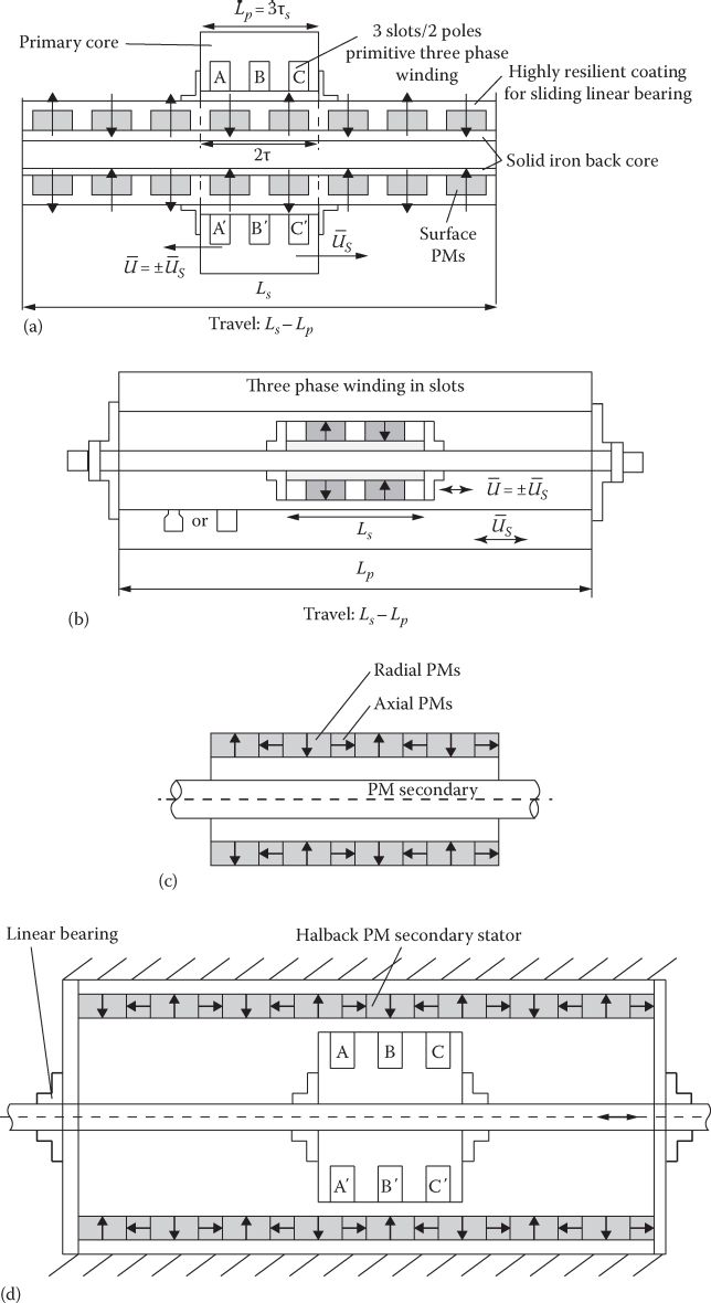
FIGURE 13.1 Basic T-LMSM topologies, (a) exterior short primary and surface PM-secondary, (b) exterior long primary stator and short PM-secondary mover, (c) Halbach PM interior secondary, (d) long Halbach PM-secondary (stator).

Images

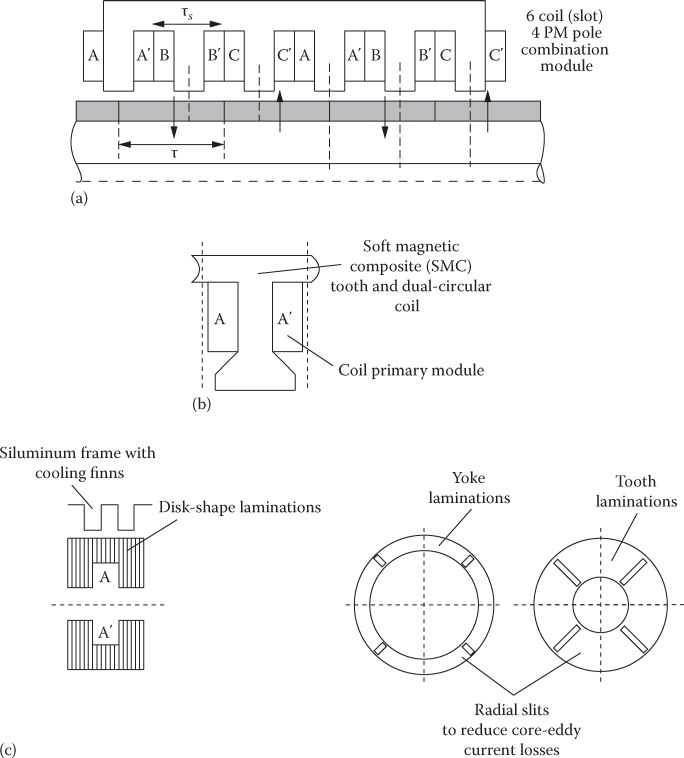
FIGURE 13.2 Six-coil (slot)/4 PM pole combination T-LPMSM (a) SMC preformed wound tooth, (b) disk-shaped lamination primary core (c).

The configurations in Figures 13.1 through 13.4 may be characterized as follows.

The long PM-secondary-stator short T-LPMSM (Figure 13.1a) is preferable when the energy consumption should be minimum while tolerance to stray PM fields is large; global initial cost tends to be larger when the travel approaches 2 ÷ 3 m; a mechanically resilient nonmagnetic coating on PM-secondary is needed for sliding-contact linear bearings fixed to the primary mover.

Images

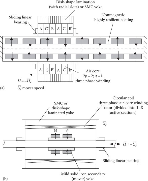
FIGURE 13.3 T-LPMSM short primary with long PM-secondary, (a) long air-core winding primary (stator) and short PM-secondary (mover) (b).

The outer-long-primary stator with interior-short-PM-secondary mover (Figure 13.1b) leads to the lowest mover weight (and highest mover acceleration) and to zero stray fields, but, unless the stator primary is supplied in a few sections, the energy consumption tends to be large. A compromise would be a 2–3 interspaced sections primary stator and PM-secondary, which is as long as one stator section plus the interspace between two stator sections. To increase the airgap flux density, thrust (by +25% or so) efficiency, axially magnetized PMs may be placed between radially magnetized ones (in a 1/2 ratio in general) in a kind of Halbach array (Figure 13.1c).

To cancel the stray PM fields but still reduce the mover weight and energy consumption, the long outer Halbach array PM-secondary stator with short primary mover may be adopted (Figure 13.1d); in not so cost-sensitive applications, this solution is worth trying; additional, insulated from shaft power aluminum bars with brushes are needed for power collection.

As the travel in T-LPMSMs is rather short (up to 3 ÷ 3.5 m at most), the pole pitch is to be small, to limit the yokes depth, for limited speed; for pitches lower than 60 mm, in general, at worst q = 1 (3 slot/pole) ac windings can be used; but, more probably, fractionary q (q < 0.5) three-phase ac windings may be applied (a 3 slot/2 PM pole combination is shown in Figure 13.1a and a 6 slot/4 PM pole module is visible in Figure 13.2a).

Images

FIGURE 13.4 T-LPMSM: generator (copper sleeve heater in an oil pumping unit to avoid paraffin formation).

Semiclosed slots lead to reduced cogging force but may be built easily only from “prefabricated” SMC teeth with the two circular phase coils already attached (Figure 13.2b). Alternatively, disk-shape laminations may be used, both in teeth and in the yokes; to reduce eddy current iron loss, when ac field transverses the yoke zones perpendicularly to laminations, and radial slits are stamped into the disk-shape laminations; four per circle is enough; the “saliency” at the laminations outer rims is to be “embedded” in the siluminum frame of primary (Figure 13.2c).

Short or long primary T-LPMSMs may be built with air-core three-phase ac winding (Figure 13.3a and b); each phase zone per pole defines the equivalent q = 1 or q < 0.5 winding type, to produce a trapezoidal or a sinusoidal emf; the air-core primary T-LPMSMs may lead to low thrust pulsations; cogging force is manifest only at primary iron yoke ends.

The T-LPMSM may be used purposely only as a generator, driven by a free-piston engine (70 ÷ 150 mm travel length), a wave energy converter, or by an oil-sucker up and down mover in an oil pumping fixture (Figure 13.4); in the latter case, the ac winding is replaced by a copper slab with solid-iron yoke mover primary.

Interpole (interior) PM-secondary for T-LPMSM (Figure 13.5) has been also investigated [1,2] but the limited yoke area at lower diameters makes it hardly adequate in terms of performance/costs; except, perhaps, for very low PM pole pitches (τ < 10 ÷ 12 mm) [3] or for larger diameters; the Halbach array surface PM-secondaries (Figure 13.1c and d) are considered in more detail in what follows as they have been proven the best solution for T-LPMSMs, where thrust density, efficiency, and mover weight are critical issues.

Images

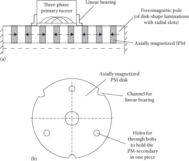
FIGURE 13.5 IPM- T-LPMSM; (a) longitudinal cross section, (b) transverse cross section.

13.2 Fractionary (q ≤1) Three-Phase AC Winding

As already mentioned, due to limited length, even limited maximum speed (6 m/s for, say, 70 mm travel in 40 Hz oscillatory motion) the pole pitch is limited and thus, except for special cases, maximum 3 slots per pole are practical (q = 1); this case is good especially for generator applications as it provides for notably smaller synchronous inductance (L_S) than the fractionary q (q ≤ 0.5) windings, because the latter exhibits a very large additional differential leakage inductance due to each armature mmf space harmonic. A smaller L_S leads to smaller voltage regulation, which is good for autonomous generators.

However, for motor-generator (drive) applications used for positioning tracking, the smaller the pole pitch (to same lower limit) the smaller the weight of the system. The rationale for choosing the primary slots count N_p and the secondary PM-poles 2p combinations developed for rotary tooth-wound PMSMs applies here as well. To avoid an “inflation” of (N_p, 2p) combinations, we will leave out most of those that have been proved to produce notable primary and secondary eddy current losses and thus have too many large sub and super speed mmf harmonics. They are governed by the rule [4]

N p = 2 p \pm 1 (13.1)

$N_{p} = 2 p \pm 1 (13.1)$

We will choose mainly those that correspond to

N p = 2 p \pm 2 or \pm 4 (13.2)

$\begin{array}{l} N_{p} = 2 p \pm 2 & or & \pm 4 \end{array} (13.2)$

Modular structures are encouraged for periodicity in linear machines that have limited longitudinal core length and thus exhibit a nonzero end effect drag force due to end teeth, if not attenuated by proper shaping of end teeth. Consequently, except for micro T-LPMSMs, which may have a short primary with only three slots and thus host three coils when a single layer winding with one coils per slot and 2p=2 or 4 is used, the following combinations are considered here, which avoid multiple coils per phase in row (as in N_p = 9, 15 …): N_p/2p = 6/4(8) (not exclusively) and multiples; N_p/2p = 12/10 and multiples of it when very small cogging force is imperative. The number of poles 2p corresponds in length to the N_p slots (teeth surrounded by coils): 2pτ = N_pτ_S.

13.2.1 Cogging Force

Cogging force manifests itself as in F-LPMSMs, and the methods to eliminate it, including the drag force, are the same for T-LPMSMs. Ultimately, when very low cogging force is required, the module may be made of N_p/2p = 6/5(7), 12/11 (13), but care must be exercised in observing the very large total synchronous inductance L_S (or L_d, L_q in IPM secondaries). The asymmetry at primary ends due to the odd number of PM poles serves to reduce the end effect drag force at zero current. Double layer windings (Figure 13.2a) are recommended to reduce the armature mmf reactive field and thus allow for larger thrust density for the given power factor. Typical winding factors for the emf (mmf fundamentals) calculated as for rotary machines, using the emf arrows diagrams [5], are given in Table 13.1. Table 13.2 shows the lowest common multiplier (LCM) of N_p and 2p, which is the number of periods of cogging force per short member length (either primary or secondary) [6]. The larger the LCM, the lower the cogging force amplitude. The almost zero mutual inductance between phases in some (N_p, 2p) combinations may be used for fault tolerant-sensitive applications.

13.3 Technical Field Theory Of T-Lpmsm

By the technical theory of T-LPMSM, we mean here a simplified 1D field theory that accounts, however approximately, for PM flux fringing in the airgap in the primary slot openings and, for IPM secondary, at its IPM’s smaller diameter.

To a first approximation, the slotting may be considered by the Carter coefficient (especially for semiclosed slots), k_C; then the radial PM airgap flux density B_g may be considered flat-topped but reduced by IPM flux fringing k_fringe and by magnetic saturation k_S coefficients[3]:

B g s P M = B r (1 - ( 2 \cdot g \cdot k C + h P M ) D i p) 1 1 + μ r e c ( g \cdot k C / τ m ) ( 1 - ( 2 \cdot g \cdot k C + h P M ) / D i p ) \cdot 1 ( 1 + k f r i n g e e ) ( 1 + k S ) (13.3)

$B_{g s P M} = B_{r} (1 - \frac{(2 \cdot g \cdot k_{C} + h_{P M})}{D_{i p}}) \frac{1}{1 + μ_{r e c} (g \cdot k_{C} / τ_{m}) (1 - (2 \cdot g \cdot k_{C} + h_{P M}) / D_{i p})} \cdot \frac{1}{(1 + k_{f r i n g e e}) (1 + k_{S})} (13.3)$

for the surface PM-secondary, and

B g s P M = B r 2 τ P M [ 1 - ( D s h / D i p ) 2 ] μ r e c [ g k C [ 1 - ( D s h / D i p ) 2 ] + ( τ P M / μ r e c ) ( τ - τ P M ) / D i p ] \cdot 1 ( 1 + k f r i n g e e ) ( 1 + k S ) (13.4)

$B_{g s P M} = \frac{B_{r}}{2} \frac{τ_{P M} [1 - {(D_{s h} / D_{i p})}^{2}]}{μ_{r e c} [g k_{C} [1 - {(D_{s h} / D_{i p})}^{2}] + (τ_{P M} / μ_{r e c}) ({τ-τ}_{P M}) / D_{i p}]} \cdot \frac{1}{(1 + k_{f r i n g e e}) (1 + k_{S})} (13.4)$

for IPM secondary.

Note: The theory in [3] was completed here by adding influence of k_C for slot opening, k_fringe for PM flux fringing, and k_s for magnetic saturation.

The slot openings’ influence is more important in IPM secondaries (as g replaces g + h_PM in SPM secondaries); the magnetic saturation influence is larger for IPMs while PM flux fringing is comparable; k_fringe can be calculated with good precision by FEM; 2D FEM suffices, as the T-LPMSM mover is placed symmetrically in the airgap. More importantly, in the presence of primary current (load), the magnetic saturation conditions change notably, especially for IPM secondaries.

In general, for well-designed T-LPMSM, k_C = 1.05 ÷ 1.25; k_fringe = 1.1 ÷ 1.2; k_S=0.10 ÷ 0.25 (for IPMs); ignoring k_fringe and k_S leads to 30 ÷ 50% errors in thrust if k_S=k_fringe = 1.22.

TABLE 13.1
Winding Factors of Concentrated Windings

Images

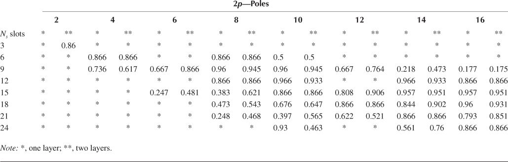
TABLE 13.2
Lowest Common Multiplier LCM of N_p and 2p

Images

Let us suppose that we extract the fundamental airgap flux density amplitude B_g₁PM and operate from now on with it, only

B g s 1 P M \approx 4 π B g P M \cdot sin π 2 (τ P M τ); B g 1 (x, t) = B g 1 P M \cdot sin (π τ x - ω 1 t); ω 1 = π τ U (13.5)

$\begin{array}{l} B_{g s 1 P M} \approx \frac{4}{π} B_{g P M} \cdot \sin \frac{π}{2} (\frac{τ_{P M}}{τ}); & B_{g 1} (x, t) = B_{g 1 P M} \cdot \sin (\frac{π}{τ} x - ω_{1} t); & ω_{1} = \frac{π}{τ} U \end{array} (13.5)$

where U is the linear speed.

As Equations 13.3 and 13.4 account for flux conservation in the presence of secondary curvature, they have to be used as they are, unless τ/D_ip < 0.1, in general (for large diameters and small pole pitches).

The emf in a primary phase E₁_a is

E 1 a = - π \cdot D i p \cdot n c \cdot k k \cdot k W 1 \cdot d d t \int 0 τ B g 1 (x, t) d x = 2 ω 1 D i p τ (k W 1 k k n c) B g 1 P M sin ω 1 t (13.6)

$E_{1 a} = - π \cdot D_{i p} \cdot n_{c} \cdot k_{k} \cdot k_{W 1} \cdot \frac{d}{d t} \int_{0}^{τ} B_{g 1} (x, t) d x = 2 ω_{1} D_{i p} τ (k_{W 1} k_{k} n_{c}) B_{g 1 P M} \sin ω_{1} t (13.6)$

E 1 a = ω 1 \cdot ψ P M \cdot sin (ω 1 t); ψ P M 1 = 2 D i p \cdot τ \cdot k W 1 \cdot k \cdot n c \cdot B g 1 P M (13.7)

$\begin{array}{l} E_{1 a} = ω_{1} \cdot ψ_{P M} \cdot \sin (ω_{1} t); & ψ_{P M 1} = 2 D_{i p} \cdot τ \cdot k_{W_{1}} \cdot k \cdot n_{c} \cdot B_{g 1 P M} \end{array} (13.7)$

Now k_k is the number of equivalent coils per phase

k_k=N_p/3 for q ≤ 0.5 modules (double layer windings)

k_k=N_p/6 for q ≤ 0.5 modules (one layer windings)

n_c is turns per one f coil

As in double layer windings (Figure 13.1), there are two coils in one slot and in one layer winding there is only one coil/slot (Figure 13.6b); the two situations are equivalent.

So the three-phase emfs are

E 1 a, b, c = E 1 2 - \sqrt sin (ω 1 t - (i - 1) 2 π 3); E 1 2 - \sqrt = ψ P M \cdot U π τ (13.8)

$\begin{array}{l} E_{1 a, b, c} = E_{1} \sqrt{2} \sin (ω_{1} t - (i - 1) \frac{2 π}{3}); & E_{1} \sqrt{2} = ψ_{P M} \cdot U \frac{π}{τ} \end{array} (13.8)$

The phase inductances may be derived rather simply for q = 1 and q ≤ 0.5 windings (Chapter 12, with πD instead of stack length etc):

L d = L q = L S = L l + l m; L m = μ 0 ( k k \cdot n c \cdot k w 1 ) 2 τ \cdot π D i p ( 1 + k f r i n g e ) p \cdot k c ( g + h P M ) (13.9)

$\begin{array}{l} L_{d} = L_{q} = L_{S} = L_{l} + l_{m}; & L_{m} = \frac{μ_{0} {(k_{k} \cdot n_{c} \cdot k_{w 1})}^{2} τ \cdot π D_{i p} (1 + k_{f r i n g e})}{p \cdot k_{c} (g + h_{P M})} \end{array} (13.9)$

for smaller PM secondaries and

L q = L l + L q m; L q m \approx μ 0 ( k k \cdot n c \cdot k w 1 ) 2 τ \cdot π D i p p \cdot k c ( g + h P M ) \cdot k q m (13.10)

$\begin{array}{l} L_{q} = L_{l} + L_{q m}; & L_{q m} \approx \frac{μ_{0} {(k_{k} \cdot n_{c} \cdot k_{w 1})}^{2} τ \cdot π D_{i p}}{p \cdot k_{c} (g + h_{P M})} \cdot k_{q m} \end{array} (13.10)$

k q m \approx (1 - τ P M τ) + 1 π sin π (1 - τ P M τ) + 1 π sin π (1 - τ P M τ) (13.11)

$k_{q m} \approx (1 - \frac{τ_{P M}}{τ}) + \frac{1}{π} \sin π (1 - \frac{τ_{P M}}{τ}) + \frac{1}{π} \sin π (1 - \frac{τ_{P M}}{τ}) (13.11)$

L d = L l + L d m; L d m = μ 0 ( k k n c k w 1 ) 2 τ \cdot π D i p ( 1 + k f r i n g e ) p \cdot k c ( 1 + τ P M 2 g τ 2 l P M ) ( 1 + k s ) (13.12)

$\begin{array}{l} L_{d} = L_{l} + L_{d m}; & L_{d m} = \frac{μ_{0} {(k_{k} n_{c} k_{w 1})}^{2} τ \cdot π D_{i p} (1 + k_{f r i n g e})}{p \cdot k_{c} (1 + \frac{τ_{P M}}{2 g} \frac{τ}{2 l_{P M}}) (1 + k_{s})} \end{array} (13.12)$

for IPM—secondaries.

k_q = 4/3 for q = 1; it may go to 1.5 for some q ≥ 0.5 windings. It may go to 1 when the mutual inductance between phases is zero (for some selected (N_p/2p) combinations).

Note: For more exact expressions of L_qm and L_dm for IPMs in Figure 13.6b, we may adopt the respective expressions obtained for segmented-secondary linear reluctance synchronous motors (Chapter 10, Equations 10.5 through 10.8, with πD instead of l_stack and axis d for q axis).

The leakage inductance comprises essentially the slot leakage component only:

L l = μ 0 π (D + h s) K k \cdot n 2 C \cdot λ s s; λ s s = h s 0 b s 0 + 2 h w b s 0 + b s + h s 3 b s (13.13)

$\begin{array}{l} L_{l} = μ_{0} π (D + h_{s}) K_{k} \cdot n_{C}^{2} \cdot λ_{s s}; & λ_{s s} = \frac{h_{s 0}}{b_{s 0}} + \frac{2 h_{w}}{b_{s 0} + b_{s}} + \frac{h_{s}}{3 b_{s}} \end{array} (13.13)$

All geometrical variables in (13.13) are visible in Figure 13.6.

Note: For double layer windings, there is some leakage-flux coupling between the adjacent coils in the same slot pertaining to different phases, but as (−i_a + i_b) varies in time its average value might be neglected. Apparently, there are no end coils in the circular shape coils of T-LPMSM; in reality, the turn average length is larger than the πD by (D + h_s)/D and thus there is additional leakage inductance in comparison with F-LPMSMs; however, its effect is notably less. We have lumped up all main flux lines in calculating L_S, L_dm, and L_qm in (13.7) through (13.9) and thus approximately, the whole inductance is considered; 2D FEM verifications are required to document this assertion thoroughly (i.e., the inclusion of different leakage inductance components). We still need the phase resistance R_S:

R S = ρ C o l C k k n C j C o I n; l c = π (D + h s) (13.14)

$\begin{array}{l} R_{S} = ρ_{C o} l_{C} \frac{k_{k} n_{C} j_{C o}}{I_{n}}; & l_{c} = π (D + h_{s}) \end{array} (13.14)$

where

ρ_Co is the copper resistivity

j_Con is the rated current density for rated RMS phase current I_n

L_C is the turn average length

k_k is the coils/phase

Images

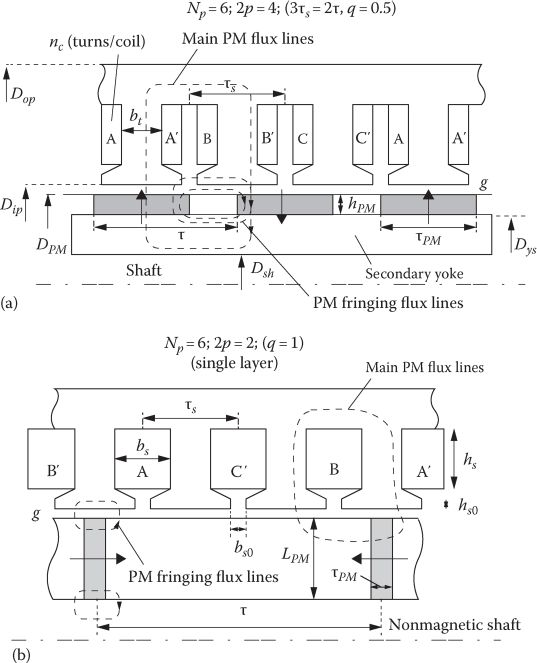
FIGURE 13.6 T-LPMSM: (a) with surface PM-secondary (N_p, 2p = 6/4, q = 0.5), (b) with IPM secondary (N_p, 2p = 6/2, q = 1).

13.4 Circuit dq Model Of T-Lpmsm

We use here the same dq model and the vector diagram as for F-LPMSMs. Let us summarize here for completeness:

V ¯ ¯ ¯ S = I S R S + d ψ ¯ ¯ S d t + j ω r ψ ¯ ¯ S; ω r = π τ k U (13.15)

$\begin{array}{l} {\bar{V}}_{S} = I_{S} R_{S} + \frac{d {\bar{ψ}}_{S}}{d t} + j ω_{r} {\bar{ψ}}_{S}; & ω_{r} = \frac{π}{τ} k U \end{array} (13.15)$

k = 1 for PM mover and k = −1 for primary mover.

ψ ¯ ¯ S = ψ ¯ ¯ P M d + L d I d + j L q I q (13.16)

${\bar{ψ}}_{S} = {\bar{ψ}}_{P M d} + L_{d} I_{d} + j L_{q} I_{q} (13.16)$

F x = 3 2 π τ [ψ P M d + (L d - L q) I d] k I q (13.17)

$F_{x} = \frac{3}{2} \frac{π}{τ} [ψ_{P M d} + (L_{d} - L_{q}) I_{d}] k I_{q} (13.17)$

G m d U d t = F x - F l o a d k - B U k; d x d t = U (13.18)

$\begin{array}{l} G_{m} \frac{d U}{d t} = F_{x} - F_{l o a d} k - B U k; & \frac{d x}{d t} = U \end{array} (13.18)$

As the equations are identical and only the expressions of ψ_PMd, L_d, L_q are different for T-LPMSMs (in contrast to F-LPMSM), there is no need to repeat here the equivalent circuits along axis d and q and, the vector diagram, the structural diagram, or the basic FOC and DTFC schemes. The airgap is considered constant, so no airgap regulation is needed or feasible. Treating eccentricity, radial or (and) axial, is not feasible with the standard dq model.

While for preliminary design and for control system design, this theory may be satisfactory, even in industry, for optimization analytical design some advanced (multilayer) field theories have been proposed (as for F-LPMSMs). They compare favorably with 2D FEM results for a notably lower computation effort but mainly for unsaturated magnetic cores in the machines.

13.5 Advanced Analytical Field Theories Of T-LPMSMs

In a few pertinent recent papers, multilayer analytical field theories of T-LPMSMs have been proposed [7,8]. The slot opening effect is considered only through the Carter coefficient, and thus the current sheet concept still holds. In [9] the entire field solution including slot openings, one by one, is considered through conformed mapping via an existing Tool Box [10]. This way in [9] the cogging force is included in the total thrust organically; again magnetic saturation is either constant or ignored. Also in [9] the magnetic equivalent circuit (MEC) analytical field theory is shown to perform worse than the multilayer + conformal mapping field theory, when both are compared with 2D FEM results.

The multilayer analytical field theory [7,8] explicitly lays out field, forces, and circuit parameters while the conformal mapping [9] avoids multilayer theory, but as it is, yields only force via Maxwell tensor. A combination of the two methods seems the way to go. Due to their high degree of generality, both methods are given some space here (one as “predictor” and the other as “corrector”). Let us consider the more general case of a quasi-Halbach PM array inner secondary with magnetic or a nonmagnetic tube (yoke) (Figure 13.7). For the ferromagnetic secondary tube (yoke), region 3 is eliminated (μ. = ∞), while for a nonmagnetic tube, region (3) holds from D_ys to longitudinal axis.

The field is periodic along axis x, but the end effect drag force may be considered by a fudge factor a posteriori placed in the thrust expression [7,8]. Due to the cylindrical symmetry, the magnetic potential holds along polar axis A(x, r, t) and must be calculated first on no load and then on load.

13.5.1 PM Field Distribution

The vector potential equations in cylindrical coordinates (Chapter 1) in the two regions (μ_rec ≈ 1 for PMs), winding + airgap and PM zones, are

\partial \partial x (1 r \partial \partial x (r A 1 θ)) + \partial \partial r (1 r \partial \partial r (r A 1 θ)) = 0; region 1 (zero currents) (13.19)

$\begin{array}{l} \frac{\partial}{\partial x} (\frac{1}{r} \frac{\partial}{\partial x} (r A_{1 θ})) + \frac{\partial}{\partial r} (\frac{1}{r} \frac{\partial}{\partial r} (r A_{1 θ})) = 0; & region 1 (zero currents) \end{array} (13.19)$

\partial \partial x (1 r \partial \partial x (r A 2 θ)) + \partial \partial r (1 r \partial \partial r (r A 2 θ)) = - μ 0 \nabla \times M ¯ ¯ ¯ (13.20)

$\frac{\partial}{\partial x} (\frac{1}{r} \frac{\partial}{\partial x} (r A_{2 θ})) + \frac{\partial}{\partial r} (\frac{1}{r} \frac{\partial}{\partial r} (r A_{2 θ})) = - μ_{0} \nabla \times \bar{M} (13.20)$

In cylindrical coordinates, the PM magnetization vector M¯¯¯ $\bar{M}$ of the quasi-Halbach array—has two components M_r and M_x:

M ¯ ¯ ¯ = M r e ¯ r + M x e ¯ x (13.21)

$\bar{M} = M_{r} {\bar{e}}_{r} + M_{x} {\bar{e}}_{x} (13.21)$

The distributions of M_r and M_x are rectangular—periodic along x (Figure 13.7b)

Images

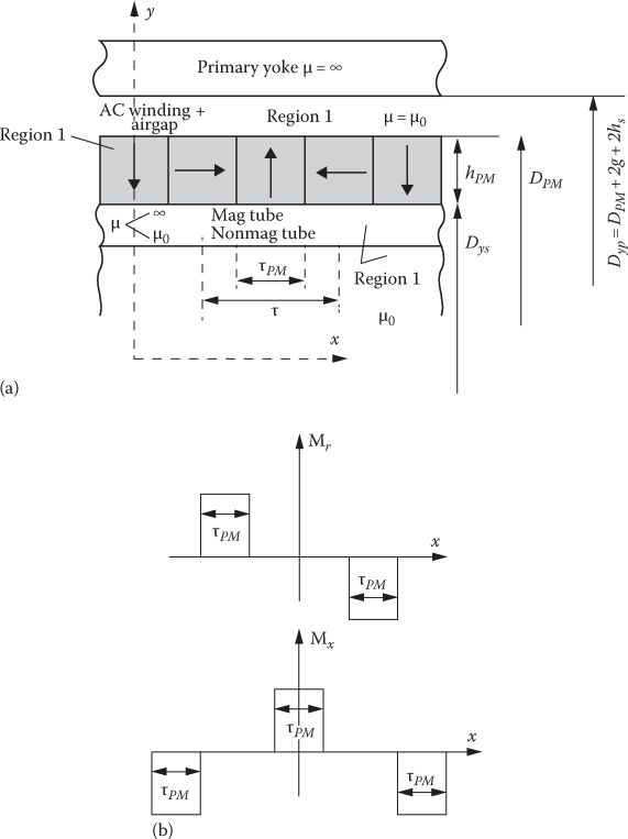
FIGURE 13.7 (a) Field layers and (b) PM magnetization vector components.

After expansion into a Fourier series

M r = \sum υ = 1, 2 \infty M r n sin (2 υ - 1 τ) π x; M x = \sum υ = 1, 2 \infty M x n sin (2 υ - 1 τ) π x; (13.22)

$\begin{array}{l} M_{r} = \sum_{υ = 1, 2}^{\infty} M_{r n} \sin (\frac{2 υ - 1}{τ}) π x; & M_{x} = \sum_{υ = 1, 2}^{\infty} M_{x n} \sin (\frac{2 υ - 1}{τ}) π x; \end{array} (13.22)$

M r n = 4 π B r μ 0 ( 2 υ - 1 ) sin (( 2 υ - 1 ) 2 π) sin (2 υ - 1) π 2 τ P M τ M x n = 4 π B r μ 0 ( 2 υ - 1 ) cos (2 υ - 1) π 2 ( τ - τ P M ) τ (13.23)

$\begin{array}{l} M_{r n} = \frac{4}{π} \frac{B_{r}}{μ_{0} (2 υ - 1)} \sin (\frac{(2 υ - 1)}{2} π) \sin (2 υ - 1) \frac{π}{2} \frac{τ_{P M}}{τ} \\ M_{x n} = \frac{4}{π} \frac{B_{r}}{μ_{0} (2 υ - 1)} \cos (2 υ - 1) \frac{π}{2} \frac{({τ-τ}_{P M})}{τ} \end{array} (13.23)$

With (13.22 and 13.23) in (13.20) the latter yields:

\partial \partial x (1 r \partial \partial x (r A 2 θ)) + \partial \partial r (1 \partial r \partial \partial r (r A 2 θ)) = \sum υ = 1 \infty P υ cos (2 υ - 1) π τ x (13.24)

$\frac{\partial}{\partial x} (\frac{1}{r} \frac{\partial}{\partial x} (r A_{2 θ})) + \frac{\partial}{\partial r} (\frac{1}{\partial r} \frac{\partial}{\partial r} (r A_{2 θ})) = \sum_{υ = 1}^{\infty} P_{υ} \cos (2 υ - 1) \frac{π}{τ} x (13.24)$

P υ = - 4 B r τ sin (2 υ - 1) π 2 sin (2 υ - 1) π 2 τ P M τ (13.25)

$P_{υ} = - \frac{4 B_{r}}{τ} \sin (2 υ - 1) \frac{π}{2} \sin (2 υ - 1) \frac{π}{2} \frac{τ_{P M}}{τ} (13.25)$

The solutions of Equations 13.19 and 13.24 depend on the nature of the secondary tube that holds the PMs; in essence, the boundary conditions are different in the two cases:

B x 1 | D y p = 0; B r 1 | D P M = B r 2 | D P M; H x 2 | D P M = 0 H x 1 | D P M = H x 2 | D P M Magnetic tube ⋮ B x 1 | D y p = 0; ⋮ B r 1 | D P M = B r 2 | D P M; B r 2 | D y s = B r 3 | D y s; A θ 3 | D = 0 = 0 H x 1 | D P M = H x 2 | D P M H x 2 | D y s = H x 3 | D y s Nonmagnetic tube (13.26)

$\begin{array}{l} {B_{x 1} |}_{D_{y p}} = 0; & {H_{x 2} |}_{D_{P M}} = 0 & ⋮ {B_{x 1} |}_{D_{y p}} = 0; & {A_{θ3} |}_{D = 0} = 0 \\ {B_{r 1} |}_{D_{P M}} = {B_{r 2} |}_{D_{P M}}; & {H_{x 1} |}_{D_{P M}} = {H_{x 2} |}_{D_{P M}} & ⋮ {B_{r 1} |}_{D_{P M}} = {B_{r 2} |}_{D_{P M}}; & H_{x 1} | D_{P M} = {H_{x 2} |}_{D_{P M}} \\ {B_{r 2} |}_{D_{y s}} = {B_{r 3} |}_{D_{y s}}; & {H_{x 2} |}_{D_{y s}} = {H_{x 3} |}_{D_{y s}} \\ Magnetic tube & Nonmagnetic tube \end{array} (13.26)$

The solutions of the field Equations 13.19 through 13.25 are now straightforward by using Bessel functions [7]:

Images

B 3 r = \sum υ = 1, 2 \infty a' 3 n ((2 υ - 1) π τ r) sin (2 υ - 1) π τ x B 3 r = \sum υ = 1, 2 \infty a' 3 n B I 0 ((2 υ - 1) π τ r) cos (2 υ - 1) π τ x Nonmagnetic tube (13.28)

$\begin{array}{l} B_{3 r} = \sum_{υ = 1, 2}^{\infty} {a^{'}}_{3 n} ((2 υ - 1) \frac{π}{τ} r) \sin (2 υ - 1) \frac{π}{τ} x \\ B_{3 r} = \sum_{υ = 1, 2}^{\infty} {a^{'}}_{3 n} B I_{0} ((2 υ - 1) \frac{π}{τ} r) \cos (2 υ - 1) \frac{π}{τ} x \\ Nonmagnetic tube \end{array} (13.28)$

B₁_r, B₁_x, B₂_r, B₂_x, have similar expressions as for ferromagnetic tube but with a′₁_n, b′₁_n, a′₂_n, b′₂_n, instead of a₁_n, b₁_n, a₂_n.

The constants F_An, F_Bn, a₁_n, b₁_n, a₂_n, b₂_n, a′₁_n, b′₁_n, a′₂_n, b′₂_n, a′_3n are found from the aforementioned boundary conditions; BI₀, BI₁ are modified Bessel functions of first kind, Bk₀, Bk₁ are modified Bessel functions of the second kind of order 0 and 1 [7];

F A n = P υ ( 2 υ - 1 ) π τ \int (2 υ - 1) π τ D y s 2 (2 υ - 1) π τ r B k 1 ( x ) B I 1 ( x ) B k 0 ( x ) + B k 1 ( x ) \cdot B I 0 ( x ) d x F B n = - P υ ( 2 υ - 1 ) π τ \int (2 υ - 1) π τ D y s 2 (2 υ - 1) π τ r B I 1 ( x ) B I 1 ( x ) B k 0 ( x ) + B k 1 ( x ) \cdot B I 0 ( x ) d x a 1 n = A 1 n C 1 n; b 1 n = B 1 n C 1 n; a 2 n = - μ r e c A 2 n C 5 n; b 2 n = - B 2 n C 10 n B n = 4 B r μ r e c ( 2 υ - 1 ) π sin (2 υ - 1) π τ (1 - τ P M τ) (13.29)

$\begin{array}{l} F_{A n} = \frac{P_{υ}}{(2 υ - 1) \frac{π}{τ}} \int_{(2 υ - 1) \frac{π}{τ} \frac{D_{y s}}{2}}^{(2 υ - 1) \frac{π}{τ} r} \frac{B k_{1} (x)}{B I_{1} (x) B k_{0} (x) + B k_{1} (x) \cdot B I_{0} (x)} d x \\ F_{B n} = \frac{- P_{υ}}{(2 υ - 1) \frac{π}{τ}} \int_{(2 υ - 1) \frac{π}{τ} \frac{D_{y s}}{2}}^{(2 υ - 1) \frac{π}{τ} r} \frac{B I_{1} (x)}{B I_{1} (x) B k_{0} (x) + B k_{1} (x) \cdot B I_{0} (x)} d x \\ a_{1 n} = \frac{A_{1 n}}{C_{1 n}}; b_{1 n} = \frac{B_{1 n}}{C_{1 n}}; a_{2 n} = - μ_{r e c} \frac{A_{2 n}}{C_{5 n}}; b_{2 n} = \frac{- B_{2 n}}{C_{10 n}} \\ B_{n} = \frac{4 B_{r}}{μ_{r e c} (2 υ - 1) π} \sin (2 υ - 1) \frac{π}{τ} (1 - \frac{τ_{P M}}{τ}) \end{array} (13.29)$

C 1 n = B I 0 ((2 υ - 1) π τ D y p 2); C 3 n = B I 1 ((2 υ - 1) π τ D P M 2); C 5 n = B I 0 ((2 υ - 1) π τ D P M 2); C 7 n = B I 1 ((2 υ - 1) π τ D y s 2); C 9 n = B I 0 ((2 υ - 1) π τ D y s 2); C 2 n = B k 0 ((2 υ - 1) π τ D y p 2) C 4 n = B k 1 ((2 υ - 1) π τ D P M 2) C 6 n = B k 0 ((2 υ - 1) π τ D P M 2) C 8 n = B k 1 ((2 υ - 1) π τ D y s 2) C 10 n = B k 0 ((2 υ - 1) π τ D y s 2) (13.30)

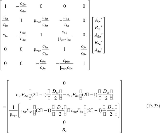
$\begin{array}{l} C_{1 n} = B I_{0} ((2 υ - 1) \frac{π}{τ} \frac{D_{y p}}{2}); & C_{2 n} = B k_{0} ((2 υ - 1) \frac{π}{τ} \frac{D_{y p}}{2}) \\ C_{3 n} = B I_{1} ((2 υ - 1) \frac{π}{τ} \frac{D_{P M}}{2}); & C_{4 n} = B k_{1} ((2 υ - 1) \frac{π}{τ} \frac{D_{P M}}{2}) \\ C_{5 n} = B I_{0} ((2 υ - 1) \frac{π}{τ} \frac{D_{P M}}{2}); & C_{6 n} = B k_{0} ((2 υ - 1) \frac{π}{τ} \frac{D_{P M}}{2}) \\ C_{7 n} = B I_{1} ((2 υ - 1) \frac{π}{τ} \frac{D_{y s}}{2}); & C_{8 n} = B k_{1} ((2 υ - 1) \frac{π}{τ} \frac{D_{y s}}{2}) \\ C_{9 n} = B I_{0} ((2 υ - 1) \frac{π}{τ} \frac{D_{y s}}{2}); & C_{10 n} = B k_{0} ((2 υ - 1) \frac{π}{τ} \frac{D_{y s}}{2}) \end{array} (13.30)$

A₁_n, B₁_n, A₂_n, B₂_n are found from the matrix:

Images

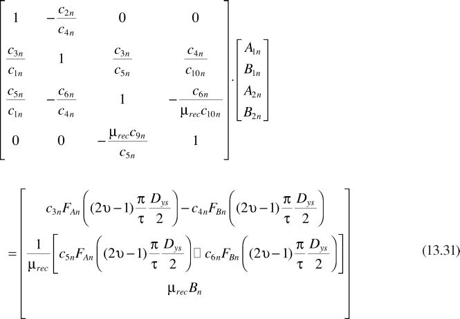
Similarly [7]

a' 1 n = A ' 1 n C 1 n; b' 1 n = B ' 1 n C 4 n; a' 2 n = - μ r e c A ' 2 n C 5 n; b' 2 n = B ' 2 n C 8 n; a' 3 n = A ' 3 n C 9 n (13.32)

$\begin{array}{l} {a^{'}}_{1 n} = \frac{{A^{'}}_{1 n}}{C_{1 n}}; & {b^{'}}_{1 n} = \frac{{B^{'}}_{1 n}}{C_{4 n}}; & {a^{'}}_{2 n} = - μ_{r e c} \frac{{A^{'}}_{2 n}}{C_{5 n}}; & {b^{'}}_{2 n} = \frac{{B^{'}}_{2 n}}{C_{8 n}}; & {a^{'}}_{3 n} = \frac{{A^{'}}_{3 n}}{C_{9 n}} \end{array} (13.32)$

with A₁_n′ , B₁_n ′, A₂_n ′, B₂_n ′, and A₃_n ′ from

Images

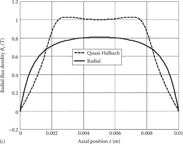
The radial flux density B_r (r=0.025 m—in the airgap) for D_yp = 0.051 m, D_pm = 0.049 m, D_ys = 0.039 m, τ = 0.01 m, τ_PM=0.006 m, B_r = 1.15 T, μ_rec = 1.05 [7] compares favorably with 2D FEM results (Figure 13.8a), and the beneficial effect of the Halback PM array is very visible in Figure 13.8b.

Similar to the aforementioned, the armature reaction and design optimization may be proceeded [7]; armature field calculation is followed by the computation of self and mutual inductances. The total force pulsations [7] shown in Figure 13.8c prove the power of the multilayer analytical method.

Images

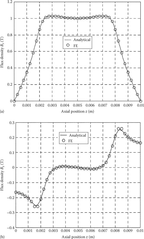
FIGURE 13.8 Radial flux density in the airgap (r=0.025 m): (a) in comparison with 2D FEM, (b) radial PMs versus Halbach array. (c) total thrust versus time. (After Wang, J. and Howe, D., IEEE Trans., MAG-41(9), 2470, 2005.)

Images

The design optimization should start with a global objective function and multiple constraints. The variables are, in general, geometric, for example: g, h_PM, τ, τ_PM, b_s₀, b_s, τ_S, and D_ys, D_PM, D_yp.

The sensitivity of performance [7] such as, efficiency, power factor, force density (N/m³ or N/kg of mover, thrust pulsations for sinusoidal current, (for a 250 N average thrust, U = 6 m/s, for τ_PM/τ=0.7) below 5% is obtained. For τ = 0.0125 m and D_PM/D_yp = 0.6, efficiency above 94% is obtained for 3 × 10⁵ N/m³ and above 60 N/kg for cos φ > 0.9 for linear thrust/current dependence up to 250 N at In=72–√ $I_{n} = 7 \sqrt{2}$ A RMS; experiments confirm the theory [7].

As the cogging force was reduced by optimization design (by optimal τ_PM/τ = 0.7 mainly), the compliance of 2D FEM with the multilayer theory for average thrust is good. Still the cogging force is not represented in the theory. The conformal method (as used in Ref. [9]) for thrust calculations shows clearly the rather notable total thrust pulsations and may be used, after optimization design through multilayer theory, to check the thrust pulsations, before 2D FEM is used for trial key verifications.

It may be argued that with 2D FEM feasible for T-LPMSMs, and, for given main geometrical parameters and current density as variables, a direct-geometric 2D FEM optimization design is now possible; true, but still to be done and proven. This is very probable for heavily saturated or small 2p T-LPMSMs.

13.6 Core Losses

As already noticed, the primary mmf is rich in space harmonics. This aspect is visible in Figure 13.9 for a 9 teeth primary (9 slot/10 pole combination). When the i_a=I_max, i_b = i_c = −I_max/2, the current sheet J_a(x) (the derivative of mmf: dF(x)/dt) is decomposed in Fourier series. For phase a only

J a (x) = \sum υ' = 1 \infty J υ' sin 2 π υ ' N p τ s (13.34)

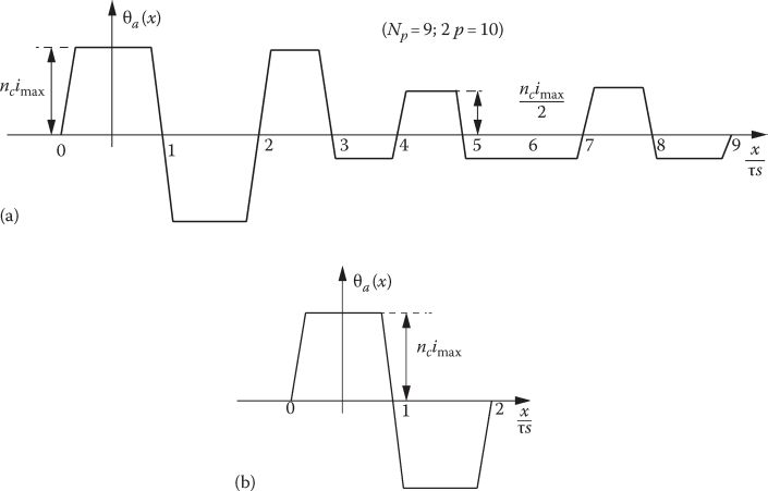
$J_{a} (x) = \sum_{υ^{'} = 1}^{\infty} J υ^{'} \sin \frac{2 π υ^{'}}{N_{p} τ_{s}} (13.34)$

Images

FIGURE 13.9 Primary three-phase mmf versus x when i_a = i_max, i_b = i_c = −i_max/2a, phase (a) only (b).

J υ' = 2 n c i τ k d υ' k p υ'; α υ' = (2 π υ ' N p τ s \times b s p 2); k d υ' = sin α υ ' α υ ' (13.35)

$\begin{array}{l} J υ^{'} = \frac{2 n_{c} i}{τ} k_{d υ^{'}} k_{p υ^{'}}; & α_{υ^{'}} = (\frac{2 π υ^{'}}{N_{p} τ_{s}} \times \frac{b_{s p}}{2}); & k_{d υ^{'}} = \frac{\sin α_{υ^{'}}}{α_{υ^{'}}} \end{array} (13.35)$

k p υ' = 2 τ N p τ s [2 sin (υ ' π N p) - sin (3 υ ' π N p)] (13.36)

$k_{p υ^{'}} = \frac{2 τ}{N_{p} τ_{s}} [2 \sin (\frac{υ^{'} π}{N_{p}}) - \sin (\frac{3 υ^{'} π}{N_{p}})] (13.36)$

Following up the calculation of the armature flux density through the multilayer theory (as in the previous paragraph), we can use Equation 13.24 of magnetic vector potential in the airgap (and PM zone) with the following boundary conditions:

B x | D y s = 0 for nonmagnetic tube; B r | D y s = 0 for magnetic support tube; H x | D y p = j y' (x) (13.37)

$\begin{array}{l} {B_{x} |}_{D_{y s}} = 0 for nonmagnetic tube; {B_{r} |}_{D_{y s}} = 0 for magnetic support tube; \\ {H_{x} |}_{D_{y p}} = j_{y^{'} (x)} \end{array} (13.37)$

B p r = - \sum υ = 1 \infty A n B I 1 (2 π υ ' τ s r) 2 π υ ' τ s cos 2 π υ ' τ s x (13.38)

$B_{r}^{p} = - \sum_{υ = 1}^{\infty} A_{n} B I_{1} (\frac{2 π υ^{'}}{τ_{s}} r) \frac{2 π υ^{'}}{τ_{s}} \cos \frac{2 π υ^{'}}{τ_{s}} x (13.38)$

B p r = \sum υ = 1 \infty A n B I 0 (2 π υ ' τ s r) 2 π υ ' τ s sin 2 π υ ' τ s x (13.39)

$B_{r}^{p} = \sum_{υ = 1}^{\infty} A_{n} B I_{0} (\frac{2 π υ^{'}}{τ_{s}} r) \frac{2 π υ^{'}}{τ_{s}} \sin \frac{2 π υ^{'}}{τ_{s}} x (13.39)$

with

A n = μ 0 J υ ' B I 0 ( ( 2 π υ ' / τ s ) D y p ) ( 2 π υ ' / τ s )

$A_{n} = \frac{μ_{0} J_{υ^{'}}}{B I_{0} ((2 π υ^{'} / τ_{s}) D_{y p}) (2 π υ^{'} / τ_{s})}$

For the other phases, similar expressions are obtained. So, implicitly, phase superposition of effects is accepted. Implicit-fixed saturation conditions are considered.

The iron losses in the primary may be calculated by the rather widely spread expressions:

P i r o n = (P h + P e + P a d) A m π D m (13.40)

$P_{i r o n} = (P_{h} + P_{e} + P_{a d}) A_{m} π D_{m} (13.40)$

where

A_m is the area where uniform flux density variation is plausible

D_m is the average diameter of that area

P h = k h f B α m; P e = 2 π σ i d 2 f 2 12 δ i \int 2 π (d B d θ e) 2 d θ e; P a d = 2 - \sqrt π k e f 3 2 \int 2 π (d B d θ) 3 2 d θ e (13.41)

$\begin{array}{l} P_{h} = k_{h} f B_{m}^{α}; & P_{e} = \frac{2 {πσ}_{i} d^{2} f^{2}}{12 δ_{i}} \int_{2 π} {(\frac{d B}{d θ_{e}})}^{2} d θ_{e}; & P_{a d} = \sqrt{2} {πk}_{e} f^{\frac{3}{2}} \end{array} \int_{2 π} {(\frac{d B}{d θ})}^{\frac{3}{2}} d θ_{e} (13.41)$

Based on the variation of airgap flux density (13.39), the peak flux density and its time (linear) variation in the primary teeth and primary yoke are calculated; this way the primary core losses may by computed based on the multilayer analytical theory [11]. Finally, the flux density distribution versus time in the primary core during steady-state operation, at different speeds U = ω₁τ/π, may be calculated by 2D FEM. The results for the example in the previous paragraph (F_x = 250 N, U = 6 m/s) are shown in Figure 13.10 [10].

Though the on load primary core losses are larger than the ones under no load, the difference is less than 15%; also, they increase almost linearly with speed; finally, at 6 m/s they are 30 W, which is about 2% of rated power (F_xU = 1500 W); the calculated efficiency [7] in the previous paragraph implies 6% of copper losses. So primary core loss under load is worthy of consideration in high efficiency T-LPMSMs. There are still the PM-secondary losses, due to slot openings and due to primary mmf space harmonics field. But the volume of the interior PM-secondary is in general less than 33% of the outer primary core volume. Thus, the PM-secondary losses are of less importance. A direct use of 2D FEM to calculate the flux density distribution and the core losses is recommended for the scope.

Images

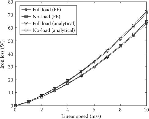
FIGURE 13.10 Primary core losses variation with speed. (After Amara, Y. et al., IEEE Trans., MAG-41(4), 989, 2005.)

13.7 Control of T-LPMSMS

By T-LPMSM control, we mean here position, speed, or thrust control for motoring and regenerative braking of direct linear motion drives. Also, a kind of different control is needed for generators with imposed sinusoidal linear motion pulsations at given mechanical frequency such as with free-piston engine prime mover (stroke in the range of 70÷150 mm, 30 Hz) or in wave energy conversion (strokes of 1÷3 m and mechanical frequency of 1÷2 Hz). Let us consider

Field oriented control (FOC)
Direct thrust and flux control (DTFC)

13.7.1 Field-Oriented Control

Due to the limited travel length (below 3 m in general) flux weakening is hardly necessary. Thus, unless an IPM secondary is used, I∗d=0 $I_{d}^{*} = 0$ in FOC. For IPM secondary, exploiting maximum thrust current condition leads to

2 I * 2 d + I * d ψ P M L d - L q = 0; L d < L q; I * d < 0 (13.42)

$\begin{array}{l} 2 I_{d}^{* 2} + I_{d}^{*} \frac{ψ_{P M}}{L_{d} - L_{q}} = 0; & L_{d} < L_{q}; & I_{d}^{*} < 0 \end{array} (13.42)$

With L_d and L_q constant, for given stator current I∗d $I_{d}^{*}$ is

I * d = ψ P M ( L d - L q ) 4 - 1 4 (ψ P M L d - L q) 2 + 8 I 2 s; - - - - - - - - - - - - - \sqrt I * d > - ∣ ∣ I ¯ S ∣ ∣ 2 \sqrt (13.43)

$\begin{array}{l} I_{d}^{*} = \frac{ψ_{P M} (L_{d} - L_{q})}{4} - \frac{1}{4} \sqrt{{(\frac{ψ_{P M}}{L_{d} - L_{q}})}^{2} + 8 I_{s}^{2};} & I_{d}^{*} > - \frac{| {\bar{I}}_{S} |}{\sqrt{2}} \end{array} (13.43)$

So, with controlled $I_{q}^{*}$ and $| {\bar{I}}_{S} |$ required, $I_{d}^{*}$ is easily calculated from (13.43); an expression that may be further simplified (see Figure 13.11); correction for magnetic saturation (with its cross-coupling effect) in IPM secondaries requires parameter online estimation and correction techniques, unless robust position control is applied.

For position tracking, a linear position sensor is necessary in general. Improving the position tracking may be approached many ways, but feed-forward or feedback disturbance observers [12] may be adequate, because in T-LPMSM not only temperature and magnetic saturation vary in time, but also the airgap, and, of course, the load. The generic FOC for T-LPMSMs, shown in Figure 13.12, is characterized by

The inclusion of a maximum thrust/current, $I_{q}^{*}$ referencer ( $I_{d}^{*} = 0$ for the surface PM secondaries); the fast thrust response and the limited travel exclude, in general, flux weakening control (maximum thrust/flux control).
A simplified online disturbance compensator based on the motion equation is included to quicken the position (and thrust) response in the presence of load force disturbance.
The PI + SM dc current regulators are considered sufficiently robust to allow—at rather low speeds—the elimination of motion voltages compensation; current limiters should be added, however.
A reference voltage limiter is added, based on dc voltage (V_dc) knowledge, to secure controlled operation; the open loop PWM allows for rather sinusoidal voltages for T-LPMSM control.
FOC may be used also for the control of an active suspension damper for cars or for a battery backup dc power source as generator. But, in this case, the position regulator is eliminated and direct current $I_{q}^{*} = 0$ control is operated based on the dc voltage and dc load current (Figure 13.13); the scheme works even for generator mode with no battery backup, but a capacitor filter, instead (Figure 13.13b).
For a wave generator, the strong variations (with position) of terminal voltages might need an additional dc–dc converter for voltage boost and stabilization. In the latter case, it is possible to use a diode rectifier (instead of PWM converter) and thus “move” the output control to the boost dc–dc converter, to yield a constant dc output voltage source from the T-LPMSM as generator (Figure 13.13b)
Direct active power and dc voltage control may replace FOC for generator mode with PWM converter.

Images

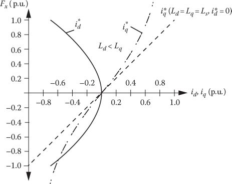
FIGURE 13.11 Maximum thrust/current conditions for IPM and SPM secondaries.

Images

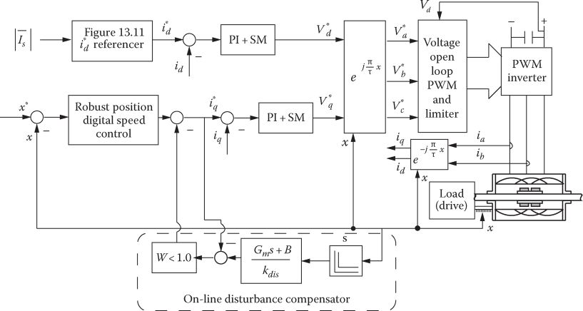
FIGURE 13.12 FOC of T-LPMSM.

Images

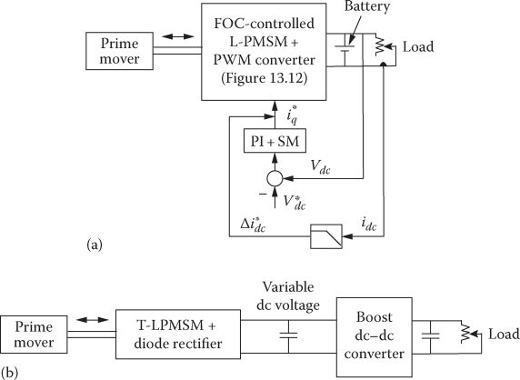
FIGURE 13.13 Generic generator T-LPMSM mode control for dc output with battery backup, (a) diode rectifier + boost dc–dc converter, (b).

13.7.2 Direct Thrust and Flux Control

When thrust control is needed, or for motion sensorless control, DTFC may be applied. As known, the cogging force may impede on control precision, vibration, and noise, and its attenuation by proper control may be achieved by a wide enough frequency band regulator of the thrust.

The cogging force versus position may be inserted as a table from FEM calculations; other force disturbance may be included also in the thrust control. However, in this case, a state observer is needed to estimate relative position $\overset{⌢}{x}$ speed $\overset{⌢}{u}$ , flux ${\overset{⌢}{ψ}}_{S}$ thrust ${\overset{⌢}{F}}_{x}$ , and dynamic force (Figure 13.14).

The state observer estimates first the stator flux ${\overset{⌢}{ψ}}_{S}$ ; only a simplified first-order delay filter is used, but a secondary order one may be put into service, to deal with the offset etc; a combined voltage–current observer may be used to work better at small speed, but the airgap (stator) irregularities would make the latter less robust. Ultimately, even the influence of airgap variation on inductance L_s may be estimated if FEM inductance/airgap curves are available.
The concept of active flux $({\bar{ψ}}_{d}^{a})$ is used here again [13]

${\bar{ψ}}_{d}^{a} = {\overset{⌢}{\bar{ψ}}}_{S} - L_{q} {\bar{I}}_{S} = [{\bar{ψ}}_{P M d} + (L_{d} - L_{q}) I_{d}] (\cos \frac{π}{τ} \overset{⌢}{x} + j \sin \frac{π}{τ} \overset{⌢}{x}) (13.44)$

${\overset{⌢}{\bar{ψ}}}_{d}^{a}$ is aligned along PM axis and thus the position $\overset{⌢}{x}$ reflects PM axis position with respect to phase a axis and thus $d \overset{⌢}{x} / d t = \overset{⌢}{u}$ , the mover speed, both in steady state and during transients, in contrast to stator flux vector speed.
The speed $\overset{⌢}{u}$ may be estimated from estimated position by a digital filter such as the PLL filter; at very low speeds, an additional speed estimation may be obtained through an observer based on motion equation and then added in a sharing mode.
Dynamic force disturbance F_dis is included to speed up the thrust (and speed) response; a simple version of it is given in Figure 13.14.
The FEM calculated function $F_{c o g} (\overset{⌢}{x})$ is stored in a table with, say, linear interpolation; another fast filter may be added here.
To attenuate the total thrust pulsations, the thrust (and flux) regulators have to be fast and robust.
For position sensorless control with_u TFC, a position regulator is added; also, to “translate” the relative estimated position ${\overset{⌢}{θ}}_{ψ_{d}^{a}}$ into an absolute one, periodic proximity sensors along the way are needed with the knowledge of where the mover is at time zero; in many applications (such as robotic surgery), relative position control is, however, sufficient.
The stator flux reference $ψ_{S}^{*}$ is made a function of thrust to yield low enough losses at small loads.
Open loop PWM of voltage with limiter provides for all available control effort at any time; flux weakening is not embedded in $ψ_{S}^{*} (F_{x}^{*})$ referencer, but the voltage limiter does its job when needed (voltage limitation).

Images

FIGURE 13.14 Generic DTFC of T-LPMSM.

Cogging force attenuation in thrust via FOC of T-LPMSM [14,15] (Figure 13.15) shows low thrust ripple, as expected, and can be “transplanted” to F-LPMSM control.

13.8 Design Methodology

Let us consider a T-LPMSM destined to pump the liquid in a limited diameter (60 mm) pipe. Trapezoidal current control is adopted as three low cost (Hall) proximity sensors are embedded in the short primary stack, for safe phase commutation; also, proximity sensors indicate braking toward end of travel.

Images

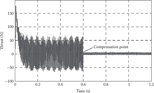
FIGURE 13.15 T-LPMSM no load thrust without and with cogging force compensator. (After Zhu, Y.-W. and Cho, Y.-H., IEEE Trans., MAG-43(6), 2537, 2007.)

The complete specifications are as follows:

Maximum outer (stator) primary diameter D_op = 60 mm

Stroke length: l_stroke = 0.3 m

Average linear speed: u_av=0.5 m/s
Mode of operation: oscillatory
Thrust: 100 N continuous duty; 175 N peak thrust (for 33% duty cycle)
V_dc = 300 V

13.8.1 Design of Magnetic Circuit

To use the pipe walls for heat dissipation, an outer primary configuration of T-LPMSM is adopted. Also, a short primary is chosen to provide high efficiency; the long PM-secondary (stroke length+ primary length) is not excessive in terms of weight and cost. To simplify the construction, disk-shaped laminations are used to build the primary core; four radial slits will reduce the core losses to small values. This implies open slots in the primary. As the average speed is low, the pole pitch should be low to allow a reasonably thin primary yoke. On the other hand, as discussed in Ref. [3], a good ratio between airgap diameter D_ip and outer diameter of primary D_oup is around 0.6 and thus D_ip ≈ 0.56 D_oup = 0.56 × 60 = 33.6 mm. Adopting a rather large peak thrust force density f_xk = 1 N/cm² (for the small airgap diameter considered), we may calculate the approximate primary length lprimary^:

$l_{p r i m a r y} = \frac{F_{x k}}{f_{x k} π D_{i p}} = \frac{175}{2 \times π \times 0 .036 \times 10^{4}} = 0.166 m (13.45)$

Now a pole pitch has to be adopted. In general, as the airgap g = 1 mm (at least) for high thrust density (without PM demagnetization) and the SPM radial depth h_PM=4 mm, the pole pitch has to be at least two times the magnetic airgap, g + h_m = 5 mm, to avoid very large PM fringing through slots openings. Consequently, we choose a 2 × 6 teeth structure with a tooth pitch τ = l_primary/6 = 13.82 mm. We may adopt a 6 slot/8 pole modular combination (2 modules), and thus the PM pole pitch τ is

$τ = \frac{6 τ_{s}}{8} = \frac{13.82 \times 6}{8} = 10.365 mm (13.46)$

For the average speed u_av=0.5 m/s, this means a fundamental frequency f₁ = u_av/2τ_PM=0.5/ (2 × 10.365 × 10⁻³) = 24.12 Hz.

The total length of PM-secondary l_secondary is

$l_{\sec o n d a r y} = l_{p r i m a r y} + l_{s t a c k} = 2 \times 0.083 + 0.30 \approx 0.47 m (13.47)$

This would mean 46 PM poles (out of which 16 are active all the time) (Figure 13.16).

To travel the 0.3 m stroke length, the time required t_s is approximated by

$t_{s} \approx \frac{l_{s t r o k e}}{U_{a v}} \times 0.85 = \frac{0.3 \times 0.85}{0.5} = 0.5 s (13.48)$

Images

FIGURE 13.16 T-LPMSM: main geometry (a) ideal currents (b).

This corresponds to t_sf₁ = 0.5 × 24=8 periods; as the acceleration to speed is considered rather fast, we may approximately consider that the T-LPMSM travels 8 periods under steady state for each stroke length.

13.8.2 Airgap Flux Density $B_{g S P M}$

According to (13.3)

$\begin{array}{l} B_{g S P M} = B_{r} (1 - \frac{(2 g k_{C} + h_{P M})}{D_{i p}}) \frac{1}{1 + μ_{r e c} (g k_{C} / τ) (1 - (2 g k_{C} + h_{P M}) / D_{i p})} \frac{1}{(1 + k_{f r i n g e}) (1 + k_{S})} \\ = 1.2 (1 - \frac{2 \times 1 \times 1.25 + 4}{33.6}) \frac{1}{1 + 1.05 \times (1 \times 1.25 / 10.365) (1 - (2 \times 1 \times 1.25 + 4) / 33.6)} \frac{1}{(1 + 0.1) (1 + 0.1)} \\ = 0.7284 T \end{array} (13.49)$

SmCo5 PMs, with B_r ≈ 1.2 T, μ_rec = 1.05 (linear demagnetization characteristic), are used to avoid corrosion effect, so typical in a pipeline.

The PM radial thickness h_PM = 4 mm and the PMs cover the whole PM pole span (τ_PM=τ); the PM fringing coefficient k_fringe=0.1 and so the magnetic saturation coefficient k_S=0.1 (despite the large total airgap (g + h_PM)), because the secondary yoke will be sized thin to reduce mover weight and cost). The Carter coefficient k_C was assigned a value of 1.25. The aforementioned analytical results may be easily verified by 2D FEM and corrected as required, to provide safe ground for the next steps in design.

13.8.3 Slot mmf for Peak Thrust

For trapezoidal current control, only two phases conduct at a time (except for phase commutation interval). In our case, that means 8 (of 12) primary coils are active (n_c turns/coil). Consequently, the thrust, written using the Lorenz force formula, is

$F_{x k} = B_{g S P M} 8 n_{c} I π D_{i p} = 0.7284 \times 8 \times π \times 0.036 \cdot n_{c} \cdot I_{p} = 0.615 \cdot n_{c} \cdot I_{p} (13.50)$

For F_xk = 175 N it follows that

$n_{c} \cdot I_{p} = \frac{175}{0.615} = 284.6 A \cdot turns/coil (13.51)$

A peak current density may be adopted after calculating the RMS value corresponding to it:

$I_{p R M S} = I_{p} \sqrt{\frac{2}{3} \times duty cycle} = I_{p} \sqrt{\frac{2}{3} \times 0.33} = 0.47 \cdot I_{p} (13.52)$

As the continuous duty cycle thrust is almost two times smaller, I_pRMS may be used for the machine design, to be valid for both situations. With current density J_Con = 8 A/mm² for I_pRMS, the cross section of a slot A_slot (which hosts two coils) is

$A_{s l o t} = \frac{2 n_{c} I_{p} \cdot 0.47}{J_{C o m} \cdot k_{f i l l}} = \frac{2 \times 284.6 \times 0.47}{8 \times 0.55} = 60.8 {mm}^{2} (13.53)$

The slot filling factor k_fill = 0.55 with preformed circular coils. But the slot width is only b_s=τ_s0.55 = 13.82 × 0.55 = 7.6 mm.

So the slot depth h_s is

$h_{s} = \frac{A_{s l o t u}}{b_{s}} + 1 = \frac{60.8}{7.6} + 1 = 9 mm (13.54)$

Now the primary yoke depth h_yp has to be verified first:

$h_{y p} = \frac{(D_{o p} - D_{i p})}{2} - h_{s} = \frac{(60 - 33.6)}{2} - 9 = 4.2 mm (13.55)$

This may seem small but as the average diameter of the primary yoke is large, D_{av yp} = D_op – h_yp = 55.8 mm, the area for yoke flux return is rather large. At no load B_yp0 is

$B_{y p o} \approx \frac{B_{g S P M} \cdot τπ D_{i p}}{π D_{a v i p} h_{y p}} = \frac{0.7284 \times 10.35 \times π \times 33.6}{π \times 55.8 \times 4.2} = 1.082 T (13.56)$

The primary peak current will produce a peak armature reaction flux density B_ap:

$B_{a p} \approx \frac{μ_{0} n_{c} I_{p}}{2 (g + h_{P M})} = \frac{1.256 \times 10^{- 6} \times 284.6}{2 (1 + 4) \times 10^{- 3}} = 35.75 \times 10^{- 3} T (13.57)$

This shows that the 4.2 mm yoke in the primary has to be kept that “large” —4.2 mm—mainly due to mechanical strength reasons. In the secondary, however, the yoke thickness h_ys is (from no load conditions)

$h_{y s} \approx \frac{B_{g P M} τπ D_{i p}}{B_{y s} π (D_{i p} - 2 h_{P M} - 2 g - h_{y s})} = \frac{0.7284 \times 10.365 \times π \times 33.6}{1.8 \times π \times (33.6 - 10 - h_{y s})} = 35.75 \times 10^{- 3} T (13.58)$

So, even with B_ys = 1.8 T the secondary yoke should be at least 7 mm thick. This leaves room for a hole (if any) in the solid back iron of secondary of only 9.6 mm.

13.8.4 Circuit Parameters

The low outer diameter of the primary (or of the pipe that holds the T-LPMSM) indicates that the tubular structure should, if used for such situations, target small thrust applications. We may now calculate the emf per phase:

$E = 4 n_{c} \cdot B_{g S P M} \cdot π \cdot D_{i p} \cdot U = 4 \times 0.7284 \times π \times 0.0336 \times 0.5 \times n_{c} = 0.4826 \times n_{c} (13.59)$

The machine inductance 2L_S for two phases in series, with its two main components, is

$2 L_{s} = 2 L_{l} + 2 L_{m p h a s e} . (13.60)$

The mutual inductances of the two phases in counter-series seem to cancel each other; this is why only L_{m phase} is considered here (k_q = 1 (13.8)):

$L_{m p h a s e} = \frac{μ_{0} \times {(4 \times n_{c} \times 0.867)}^{2} \times 0.010365 \times π \times 0.0336 \times (1 + 0.15)}{2 \times 8 \times 1.25 \times (1 + 4) \times 10^{- 3}} = 0.7687 \times 10^{- 6} n_{c}^{2} (13.61)$

From (13.11)

$L_{l} = μ_{0} π (D_{i p} + h_{s}) 4 \cdot n_{c}^{2} \cdot λ_{s s} = μ_{0} π (0.0365 + 0.009) \times 4 \times 0.6158 \times n_{c}^{2} = 0.442 \times 10^{- 6} \times n_{c}^{2} (13.62)$

With λ_ss

$λ_{s s} = \frac{1}{b_{s}} + \frac{h_{s} - 1}{3 b_{s}} = \frac{1}{7.6} + \frac{8}{3 \times 7.6} \approx 0.6158 (13.63)$

Finally, from (13.12)

$R_{s} = ρ_{c_{o}} \cdot \frac{l_{c} 4 n_{c}^{2} J_{C o n}}{I_{n} n_{c}} = \frac{2.1 \times 10^{- 8} \times π (0.0365 + 0.009) \times 4 \times 8 \times 10^{6}}{140} \times n_{c} = 6.857 \times 10^{- 4} \times n_{c}^{2} (13.64)$

13.8.5 Number of Turns per Coil n_c (All Four Circular Shape Coils per Phase in Series)

The two phases in conduction equation are

$V_{d c} = 2 R_{s} i + 2 E + 2 L_{s} \frac{d i}{d t} (13.65)$

In order to provide flat top current at U = 0.5 m/s for peak thrust, current chopping has to be allowed; if the hysteresis band of current control is 5% of peak current and the switching frequency in the PWM converter fs = 10 kHz Equation 13.65 becomes (for V_dc = 300 V)

$\begin{array}{l} 300 = (2 \times 6.857 \times 10^{- 4} 284 + 2 \times 0.4826 + 2 \times (0.7687 + 0.442) \times 10^{- 6} \times 0.05 \times \frac{284}{10^{- 4}}) \cdot n_{c} \\ = (0.38076 + 0.9652 + 0.34173) \cdot n_{c} \end{array} (13.66)$

So the number of turns per coil n_c = 178 turns/coil.

The wire gauge is obtained from

$d_{w i r e} = \sqrt{\frac{4}{π} \frac{I_{n}}{J_{C o n}}} = \sqrt{\frac{4}{π} \frac{(n_{c} I_{n} / n_{c})}{J_{C o n}}} = \sqrt{\frac{4}{π} \frac{(274 / 2) / 178}{8 \times 10^{- 6}}} \approx 0.36 mm (13.67)$

The rated current

$I_{n} = (284 / 2) / n_{c} = (284 / 2) / 178 = 0.8 A (13.68)$

13.8.6 Copper Losses and Efficiency

The rated losses p_Con are

$p_{C o n} = 2 R_{s} I_{n}^{2} = 2 \times 6.857 \times 10^{- 4} \times 178^{2} \times {0.8}^{2} = 27.8 W (13.69)$

The electromagnetic P_elm power

$P_{e l m} = F_{x n} \cdot U = 100 \times 0.5 = 50 W (13.70)$

So, neglecting other losses, the efficiency would be

$η_{n} = \frac{P_{e l m}}{P_{e l m} + p_{C o n}} = \frac{50}{50 + 27.8} = 0.6426 (13.71)$

The electric time constant

$T_{e} = \frac{L_{s}}{R_{s}} = \frac{1.21 \times 10^{- 6} \times n_{c}^{2}}{6.857 \times 10^{- 4} \times n_{c}^{2}} = 1.765 \times 10^{- 3} s (13.72)$

This small time constant indicates that, for efficient (low band width) current chopping, at least 10 kHz switching frequency is required.

Note: The performance may seem acceptable at this low speed (0.5 m/s) but still other linear PM motors—with higher frequency (as those treated in the next chapter)—have to be investigated for small speeds, in tubular but especially in flat LPMSM configurations.

Once a preliminary design attempt has been made, an optimization design should follow; finally, 2D FEM key verifications or direct geometrical optimization refinements may be performed; all these tasks are, however, beyond our scope here.

13.9 Generator Design Methodology

Free-piston energy converters such as Stirling engines [22] may be used in series HEVs [16,17]. Also, wave energy conversion through T-LPMSMs, despite 0.5–1.0 m/s speeds and powers up to hundreds of kW for travel length of 3 ÷ 4 m or for smaller powers (10–15 kW), have been proposed recently [16–22]. Both flat and tubular LPMSMs have been investigated for the scope. Moreover, T-LPMSMs have been proposed for low frequency active dampers in cars [21].

Using two (three)-phase T-LPMSMs is natural for travels that go well above 6 ÷ 10 pole pitches (above 30 mm in general). In what follows the case of a linear wave—energy generator is approached due to its potential (7 kW mechanical power capacity for 1 m of sea shore around Japan, e.g., [20]).

The challenges are related to the low speed and super high thrust levels encountered. The tubular structure—with its ideally zero resultant radial force on the mover—makes it suitable for the scope. Let us consider a super large power (250 kW, 1 m/s), such as a case study, starting from Ref. [29], where, however, cogging force is investigated in a double-sided flat LPMSG.

The design has quite a few critical issues to tackle, such as small surface thrust density in N/cm² is not enough to build an economically viable solution; in our view, at least 6 ÷ 7 N/cm², even 9 ÷ 10 N/cm², would be more adequate. Such a high thrust density comes with two heavy “prices”:

A sizeable quantity of PMs and copper losses
Large voltage regulation, which impedes the inverter kVA ratings

It is decided here, as a compromise, to choose a surface PM configuration (due to high thrust density) and low inductance.

The mechanical airgap for such an application should not go below g = 3 mm. To avoid PM demagnetization and provide for large thrust, the radial thickness of the PMs should be h_PM ≥ 12 mm. But the slot pitch should be large enough to allow a small enough PM flux fringing. For that, τ_s > 40 mm. Let us consider τ_s=60 mm; in this case, a tentative primary frequency at U_n = 1 m/s is

$f_{n i} \approx \frac{U_{n}}{2 τ} > \frac{1}{2 \times 0.06} \approx 8.33 Hz (13.73)$

As τ ≠ τ_s this is only an orientative value.

This is rather low frequency especially for the three-phase PWM converter but still perhaps acceptable.

Let us consider f_xn=6 N/cm²; efficiency η_n=0.85 (due to very small speed); the total thrust F_xn is

$F_{x n} = \frac{(P_{n} / η_{n})}{U_{n}} = \frac{250 \times 10^{3} / 0.85}{1} = 294 kN (13.74)$

Therefore, the total short primary outer stator area A_airgap is

$A_{a i r g a p} \approx \frac{F_{x n}}{f_{x n}} = \frac{294 kN}{6 \times 10^{4}} = 4.9 m^{2} (13.75)$

With an airgap diameter D_ip = 1.1 m, the length of the primary l_primary is

$l_{p r i m a r y} = \frac{A_{i r g a p}}{π D_{i p}} = \frac{4.9}{π \times 1.1} = 1.42 m (13.76)$

Now we have to choose the number of short primary (stator) teeth:

$N_{p} = Integer (\frac{l_{p r i m a r y}}{τ_{s}}) = Integer (\frac{1.42}{0.06}) \approx 24 (13.77)$

To reduce cogging force, we may choose two modules of 12 slots (teeth) with 14 PM poles (each). Therefore, we do have 24 teeth in the short primary (stator) that correspond to 28 PM poles (per same total length). So the PM pole pitch τ_PM, which in fact defines the primary frequency, is

$τ_{P M} = τ_{s} \times \frac{24}{28} = 60 \times \frac{24}{28} = 51.43 mm (13.78)$

To further reduce the cogging force, the PM span/PM pole pitch is optimized first; then the two primary halves of 12 teeth/14 PM poles may be shifted optimally by about τ_PM/6, in general.

Still to be decided is if open slots may be used; here lies another compromise: open slots lead to large cogging force but semiclosed slots, which lead to smaller cogging force, experience large PM fringing (lower thrust) and higher leakage (and total) machine inductance.

Even if the frequency f_nf

$f_{n f} = \frac{U_{n}}{2 τ_{P M}} = \frac{1}{2 \times 0.05143} = 9.72 Hz (13.79)$

the armature reaction I_nL_s/ψ_PM ratio decides the power factor of the machine; ψ_PM is the PM flux linkage in a phase; with large force density I_nL_s increases, and thus a large L_s may not be tolerable. So, as the h_PM + g = 12 + 3 = 15 mm, it is felt here that, with a stator tooth width of b_t = 35 mm, and a slot width b_s= τ_s – b_t=60–35 = 25 mm, the PM span/PM pole pitch may be 40/51 = 0.77 and thus a good compromise may be achieved. Only 2D FEM key verifications could lead to an optimal solution here, based on a comprehensive fitting (objective) function. The design here serves only as a hopefully realistic start-up (Figure 13.17).

With strong PMs of the future (B_r = 1.4 T, µ_rec = 1.07), already in the labs the airgap flux density produced by PMs may be calculated here ignoring the PM-secondary curvature (D_ip) >> (g + h_PM):

$B_{g P M} = B_{r} \cdot \frac{h_{P M}}{h_{P M} + g} \cdot \frac{1}{(1 + k_{f r i n g e})} \cdot \frac{1}{(1 + k_{s})} (13.80)$

Images

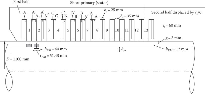
FIGURE 13.17 Large T-LPMSM generator geometry.

Images

FIGURE 13.18 Star of emfs 12 coil/14 pole combination.

Magnetic saturation should not be very influential because the magnetic airgap (h_PM + g) is large, despite large primary mmf (to secure high thrust density); so with k_s = 0.10 and with k_fringe = 0.10 (open slots), the airgap average PM flux density is

$B_{g P M} = 1.4 \times \frac{12}{12 + 3} \times \frac{1}{1 + 0.1} \times \frac{1}{1 + 0.1} = 0.925 T (13.81)$

More PM height (and weight) would produce higher B_gPM but, since the cost of PMs is high, it is not easy to justify the PM extra cost by a modest thrust (and efficiency) improvement. There are two neighboring coils per phase in series (in general) for 12 coils/14 poles module configuration (Figure 13.18).

The fundamental winding factor k_wi for 12 coil/14 PM poles combination is k_w₁ = 0.933 and can be easily inferred from Figure 13.18 (it is as for q=2!). Now the peak PM flux per one-phase coils is

$ϕ_{P M} \approx B_{g P M} \frac{b_{P M}}{2} π D_{i p} k_{w_{1}} (13.82)$

This is equivalent to calculating the emf per phase with the formula

$E_{\max} = 16 B_{g P M} \cdot π \cdot D_{i p} n_{c} \cdot k_{w_{1}} U = 16 \times 0.925 \times π \times 1.1 \times 0.933 \times 1 \times n_{c} = 352 \times n_{c} (13.83)$

In addition, the thrust F_xn is simply

$F_{x n} = \frac{3}{2} B_{g P M} π D_{i p} \times 16 I_{n} \sqrt{2} = \frac{3}{2} \frac{π}{τ} ψ_{P M} I_{q}; I_{q} = I_{n} \sqrt{2}; I_{d} = 0 (13.84)$

Zero I_d control secures maximum thrust/current and also lagging power factor, as needed for the PWM converter boosting mode required to control power generating.

$294 \times 10^{3} = \frac{3}{2} \times 0.925 \times π \times 1.1 \times 16 \times 0.933 \times \sqrt{2} \times I_{n} n_{c} (13.85)$

So the mmf coil (RMS value) I_n · n_c is

$I_{n} n_{c} \approx 2.915 \times 10^{3} A turns (RMS) (13.86)$

The slot width is only 25 mm and there are 2 coils in a slot; so the required area A_slot is

$A_{s l o t} = \frac{2 I_{n} \cdot n_{c}}{j_{C o n} \cdot k_{f i l l}} = \frac{2 \times 2.915 \times 10^{3}}{3 \times 0.55} = 3532 {mm}^{2} (13.87)$

So the slot height h_s is

$h_{s} = \frac{A_{s l o t}}{b_{s}} + 2 = \frac{3532}{25} + 2 = 143 mm (13.88)$

This is close to the acceptable limit, typical for large generators but as h_s/b_s = 143/25 = 5.65 < (6 ÷ 7), the slot leakage inductance will be notable, though.

The copper losses for rated thrust p_Con are

$p_{C o n} = 3 ρ_{C o} \frac{l_{c} 16 n_{c}^{2} J_{C o n}}{I n_{c}} = 3 \times 2.1 \times 10^{- 8} \times π \times (1.1 + 0.143) \times 16 \times 58.3 \times 3 \times 10^{6} = 68.9 kW (13.89)$

So, neglecting all other losses the efficiency would be

$η_{n} \approx \frac{P_{n}}{P_{n} + p_{C o n}} = \frac{250}{250 + 68.9} = 0.784 (13.90)$

This is not the expected 85%; some improvements may be obtained by decreasing further the current density and thus deepening the slots; but the gain will perhaps be up to 80%. It is possible to get better efficiency by adopting a smaller specific thrust f_xn, and thus for a larger diameter machine an even higher initial cost of the system is obtained. The machine inductance per phase with three active phases (sinusoidal (vector) current control) is

$L_{s} = L_{l} + L_{m} (13.91)$

$L_{m} = \frac{3}{2} \frac{4 n_{c}^{2} b_{P M} π D_{i p} μ_{0}}{g + h_{P M}} = 1.256 \times 10^{- 6} \times \frac{3}{2} \times \frac{4 \times 0.04 \times π \times 1.1 \times n_{c}^{2}}{(3 + 12) \times 10^{- 3}} = 0.0694 \times 10^{- 3} \times n_{c}^{2} (13.92)$

$\begin{array}{l} L_{l} = 16 \cdot μ_{0} n_{c}^{2} π (D_{i p} + h_{s}) λ_{s s} = 16 \times 1.256 \times 10^{- 6} \times 3.14 \times (1.1 + 0.143) \times 1.96 \times n_{c}^{2} \\ = 0.1537 \times 10^{- 3} \times n_{c}^{2} \end{array} (13.93)$

$\begin{array}{l} λ_{s s} \approx \frac{h_{s}}{b_{s}} + \frac{b_{s 0}}{b_{s}} = \frac{14}{3 \times 25} + \frac{2}{25} = 1.96 \\ L_{s} = (0.1537 + 0.0694) 10^{- 3} \times n_{c}^{2} = 0.2231 \times 10^{- 3} \times n_{c}^{2} \end{array} (13.94)$

$\frac{L_{s} I_{n} \sqrt{2}}{E_{\max} / ω_{r}} = \frac{0.2231 \times 10^{- 3} \times n_{c}^{2} \times I_{n} \sqrt{2}}{352 \times n_{c}} = \frac{0.2231 \times 10^{- 3} \times \sqrt{2} \times 2915 \times 2 \times π \times 9.72}{352} = 0.159 (13.95)$

This is a rather small value, which means that the power factor is going to be very good; so the inverter kVA rating will be acceptable. Increasing the slot depth in order to increase efficiency, at the cost of a larger machine (primary), will also diminish the power factor; but since it is rather high, such a cost may be acceptable.

Note: The two design examples treat rather extreme specifications to test the capabilities of T-LPMSMs and are to be considered as preliminary sizing, start-up solutions.

13.9.1 Generator Control Design Aspects

The generator mode control depends heavily on the application. However, field oriented control (FOC) with pure I_q control is appropriate as it secures lagging power factor, and thus the PWM converter works as a forced commutation mode rectifier, which corresponds to the needed voltage boosting mode.

Figure 13.19a shows the autonomous generator mode with dc output load, where dc voltage control with current limiter may be appropriate to offer the reference current $I_{q}^{*}$ ; as the speed varies, the influence of $I_{q}^{*}$ control on output power changes and thus some emf compensation in FOC is required. When the output dc voltage of T-LPMSM as generator is controlled from outside (Figure 13.19b), the control of the dc output current seems more adequate for T-LPMSG; as dc voltage is constant, or only slightly variable, the output power control is handled well through $I_{d c}^{*}$ control.

As linear generators are characterized by oscillatory linear motion with large amplitude (which needs 6–10 pole travel length or more and thus imposes three-phase configurations), the power delivered over the travel length varies notably and the PWM converter has to be designed and controlled to handle the situation; a fixed dc voltage might not allow full energy extraction and thus an intermediary dc–dc converter with variable (controllable) boost ratio might be necessary.

In applications such as “active suspension damper” with a travel of about 0.2 m in car applications, the thrust control—through $I_{q}^{*}$ —should be directly commanded from the suspension supervision system.

Images

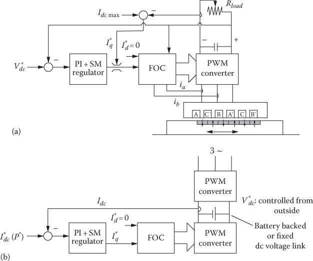
FIGURE 13.19 Typical generator control systems (a) for nonfixed dc link voltage (dc voltage control), (b) for fixed dc link voltage.

13.10 Summary

The tubular configuration for L-PMSMs is characterized by ideally zero radial force on the mover, low copper losses due to the circular shape of the coils, and better heat transmission from coils to primary core due to their contact along the entire coil length.
Due to mechanical reasons, the tubular configuration is limited to a travel of at most 3 ÷ 4 m.
T-LPMSM applications range from free-piston thermal engine generators to wave energy converters and active suspension dampers for cars or linear position tracking from more than 0.3 m to 3 m travel length.
The three-phase windings, supplied from off the shelf PWM converters used for rotary ac machines, are connected for q = 1 slot/pole/phase or for fractionary q (q ≤ 0.5) winding configurations to allow a small enough pole pitch and thus reduce the machine weight and initial cost; a travel of more than 6 ÷ 10 pole pitches (PM pole pitches) justifies the use of T-LPMSMs.
The primary iron core may be made of prefabricated soft magnetic composite (SMC) teeth (with two circular coils attached)—when the “slots” may be semiclosed (adequate for IPM secondaries)—or can be fabricated from disk-shaped laminations with three (four) radial slits, to reduce core losses in the yoke zone.
Air-core three-phase windings (with circular coils) assembled: in q = 1 or q ≤ 0.5 winding configurations may be used when thrust pulsations are a sensitive issue, though the thrust/weight and efficiency tend to be smaller than those in iron core configurations.
The fundamental winding factor of q ≤ 0.5 windings is large, but their mmfs are rich in space harmonics and, consequently, the secondary (PM and yoke) eddy currents tend to be larger; however, as long as the fundamental frequency is below 50 Hz, their contribution to total losses is less than 5% in general.
A technical 1D field theory is developed and shown to allow preliminary realistic performance assessment.
A 2D multilayer analytical field theory is presented in notable detail and compared with 2D FEM results; slot openings are considered by conformal mapping method. Apart from magnetic saturation all other major phenomena are correctly portrayed by the analytical multilayer theory for notably less computation effort; so optimization analytical design may be approached this way; finally, around “analytical” optimum configuration a direct geometrical FEM optimization may be executed for final refinements.
The cogging force may be reduced as for F-LPMSMs, mainly by optimizing the PM span/PM pole pitch and (q ≤ 0.5) fractionary windings; also by making the whole primary of displaced modules or the PM-secondary of displaced poles. Still the end teeth drag force at zero current has to be reduced by dedicated design procedures; alternatively, it may be calculated by 2D FEM and considered a known disturbance, to be handled by the thrust (or current I_q) control.
Core losses may be approached by 2D FEM (or a multilayer analytical method for magne-tostatic field distribution, with widely accepted analytical formulae).
The T-LPMSM may be field oriented controlled (FOC) when zero $I_{d}^{*}$ (or maximum thrust/current for IPM secondary) control seems appropriate as flux weakening is not very probable due to small maximum speed (6 m/s or so).
Cogging force may be treated as a disturbance, to be compensated through the $I_{q}^{*}$ control.
The generator control depends on the application; if the dc output voltage is controlled from other source, then a forced—commutation rectifier is field oriented controlled (FOC) in the sense that the reference current $I_{q}^{*}$ is the output of the dc output current closed loop regulator for the given output power reference.
It is also feasible to use for generator control a diode rectifier with a variable output—voltage and a constant dc output voltage dc–dc converter.
Direct thrust and flux control (DTFC) is also used for T-LPMSMs, especially when thrust pulsations should be reduced drastically or when motion—sensorless control is performed.
Two case studies for T-LPMSM design have been performed, both of small speed (≤1 m/s) but one for small thrust (100 N) for motoring and one of 294 kN for generating. For the first case, the thrust density was 1 N/cm², while for the other it was 6 N/cm². At such small speeds, the efficiency is only above 64% in the first case and 78.8% for the second case, as a compromise between performance and T-LPMSM weight (and initial cost). New linear PM generator design efforts for ocean energy conversion are surfacing by the day [23].
Linear magnetic gears have been incorporated recently into T-LPMSM for better performance at very low linear speed [24,25] or as magnetic screws [26].

References

1. I. Boldea and S.A. Nasar, Linear Electric Actuators and Generators, Chapter 4, Cambridge University Press, Cambridge, U.K., 1997.

2. J. Wang, G.W. Jewell, and D. Howe, A general framework for the analysis and design of tubular linear PM machines, IEEE Trans., MAG-35(2), 1999, 1986–2000.

3. N. Bianchi, S. Bolognani, D.D. Corte, and F. Tonel, Tubular linear PM motors: An overall comparison, IEEE Trans., IA-39(2), 2003, 466–475.

4. E. Fornasiero, L. Albanti, N. Bianchi, and S. Bolognani, Consideration on selecting fractional-slot windings, Record of IEEE-ECCE-2010, Atlanta, GA, 2010, pp. 1376–1383.

5. N. Bianchi, M.D. Pre, G. Grezzoni, and S. Bolognani, Design considerations on fractional slot fault-tolerant synchronous motors, IEEE Trans., IA-42(4), 2006, 997–1006.

6. I. Boldea, Electric Generators Handbook, Vol. 2: Variable Speed Generators, Chapter 11, CRC Press, Taylor & Francis, New York, 2006.

7. J. Wang and D. Howe, Tubular modular PM machines equipped with quasi-Halbach magnetized magnets—Part I + II, IEEE Trans., MAG-41(9), 2005, 2470–2489.

8. N. Bianchi, Analytical computation of magnetic fields and thrust in a tubular PM linear servo motor, Record of IEEE-IAS-2000, Rome, Italy, 2000.

9. D.C.J. Krop, E.A. Lomonova, and A.J.A. Vandenput, Application of Schwarz-Cristoffel mapping to PM linear motor analysis, IEEE Trans., MAG-44(3), 2008, 352–359.

10. T.A. Driscoll, Schwarz-Cristoffel toolbox user’s guide: Version 2.3, Department of Mathematical Sciences, University of Delaware, Newark, DE, 2005.

11. Y. Amara, J. Wang, and D. Howe, Stator iron losses of tubular PM motors, IEEE Trans, MAG-41(4), 2005, 989–995.

12. I. Boldea and S.A. Nasar, Electric Drives, 2nd edn., Chapter 7, CRC Press, Taylor & Francis, New York, 2006.

13. I. Boldea, C. Paicu, and G.D. Andreescu, Active flux concept in sensorless unitary ac drives, IEEE Trans., PE-23(5), 2008, 2612–2618.

14. H.-W. Kim, J.-W. Kim, S.-K. Sul, Thrust ripple free control of cylindrical linear synchronous motor using FEM, Record of IEEE IAS-1996, Annual Meeting, New Orleans, LA, vol. 1, 1996.

15. Y.-W. Zhu and Y.-H. Cho, Thrust ripple suppression of PM linear synchronous motor, IEEE Trans., MAG-43(6), 2007, 2537–2539.

16. W.R. Cawthorne, Optimization of brushless PM linear alternator for use with a linear internal combustion engine, PhD Thesis, West Virginia University, Morgantown, WV, 1989.

17. J. Lim, H.-Y. Choi, S.-K. Hong, D.-H. Cho, and H.-K. Jung, Development of tubular type linear generator for free-piston engine, Record of ICEM-2006, Chania, Greece, 2006.

18. V. Delli Colli, P. Cancelliere, F. Marignetti, R. Di Stefano, and M. Scarano, A tubular generator drive for wave energy conversion, IEEE Trans., IE-53(4), 2006, 1152–1159.

19. J. Faiz, M.E. Salari, and Gh. Shahgholian, Reduction of cogging force in linear permanent magnet generators, IEEE Trans., MAG-46(1), 2010, 135–140.

20. K. Hatakenaka, M. Sanada, and Sh. Morimoto, Output power improvement of PM-LSG for wave power generation by Halbach permanent magnet array, Record of LDIA-2007, 2007.

21. I. Boldea and S.A. Nasar, Linear Motion Electromagnetic Devices, Chapter 4, Taylor & Francis, New York, 2001.

22. P. Zheng, A. Chen, P. Thelin, W.M. Arshad, and Ch. Sadarangani, Research on a tubular longitudinal flux PM linear generator used for free-piston energy converter, IEEE Trans., MAG-43(1), 2007, 447–449.

23. J. Prudell, M. Stoddard, E. Amon, T.K.A. Brekken, and A. von Jouanne, A PM tubular linear generator for ocean wave energy conversion, IEEE Trans., IA-46(6), 2010, 2392–2400.

24. S. Niu, S.L. Ho, and W.N. Fu, Performance analysis of a novel magnetic-geared tubular linear PM machine, IEEE Trans, MAG-47(10), 2011, 3598–3601.

25. R.C. Holehous, K. Atallah, and J. Wang, Design and realization of a linear magnetic gear, IEEE Trans., MAG-47(10), 2011, 4171–4174.

26. J. Wang, K. Atalah, and W. Wang, Analysis of a magnetic screw for high force density linear electromagnetic actuators, IEEE Trans., MAG-47(10), 2011, 4477–4480.

..................Content has been hidden....................

You can't read the all page of ebook, please click here login for view all page.

Table of Contents for Chapter 13 Tubular Linear Permanent Magnet Synchronous Motors

Create new playlist

Sign In

Sign Up

Table of Contents for
Chapter 13 Tubular Linear Permanent Magnet Synchronous Motors