Chapter 25. Humidification and Drying

Search in book...
Toggle Font Controls
Create new playlist

Name your new playlist

Playlist description (optional)
Sign In

Email address

Password

Forgot Password?

or

Continue with Facebook

Continue with Google
Sign Up

Full Name

Email address

Confirm Email Address

Password

or

Continue with Facebook

Continue with Google

Chapter 25. Humidification and Drying

Learning Objectives

After completing this chapter, you will be able to:

Understand the process of humidification and the simultaneous heat and mass transfer involved in that process.
Explain the basis of operation of a cooling tower.
Develop and solve simple models for sizing a cooling tower.
Understand different mechanisms for drying of a solid, the so-called constant rate versus falling rate periods.
Calculate the moisture content versus time during a batch drying process.
Examine the role of pore diffusion versus capillary flow in drying of solids.

Processes where simultaneous heat and mass transfer occur is common in chemical process industries. The simplest example is evaporation from a pool of water to relatively dry air. The definitions of dry (air temperature) and wet (water temperature) bulb temperatures are important in this context; this is the first topic examined here. The evaporation causes some cooling of the water to supply the latent heat of evaporation. This causes the water temperature to be lower than the air temperature. This cooling phenomena is commonly used to cool hot water from process streams by contacting it with air. This is the basic principle of operation of a cooling tower. We will study how the principles of heat and mass transfer can be used to design this equipment.

Drying of a wet solid is another example of simultaneous heat and mass transfer. This is a commonly practiced unit operation and one of the most energy intensive processes. Hence an understanding of the transport processes in drying is a prerequisite to energy optimization and the design of next-generation drying equipment. The chapter also provides an overview of different mechanisms of moisture transport from the solid being dried to the gas phase.

25.1 Wet and Dry Bulb Temperature

Wet bulb and dry bulb thermometers provide a means to measure the moisture content of air. In the simplest form, a wet bulb thermometer is an ordinary thermometer covered with a wetted wick. The water evaporation causes the wet bulb to cool and the temperature recorded by this thermometer is different from that measured by one with a dry bulb. In this section we model a system based on simultaneous heat and mass transfer considerations and show how the temperature difference between the dry and wet bulbs is related to the moisture content of the air. The system modeled is shown schematically in Figure 25.1.

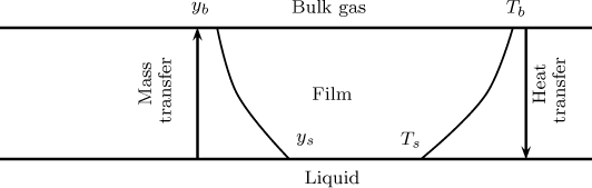
A schematic diagram showing the heat transfer and mass transfer during the process of evaporation.

Figure 25.1 Schematic of heat and mass transfer from an evaporating surface. Note: Profiles would be modeled as a linear function for the low flux mass transfer case.

The mass transfer rate (liquid to gas) is calculated using a mass transfer coefficient, $k_{m}^{o}$ $k_{m}^{o}$ , assuming a low flux model. The mole fraction of vapor corresponds to the saturation condition at the surface, denoted by y_s, and the mole fraction in the gas is y_b. Hence the mass transfer or evaporation rate is

N_{A} = k_{m}^{o} C (y_{s} - y_{b})

$N_{A} = k_{m}^{o} C (y_{s} - y_{b})$

Here y_s is the equilibrium mole fraction at the interface, which depends on T_s. Note y_s = P_vap(T_s)/P, where P_vap is the vapor pressure and P is the total pressure.

Heat transfer from gas at a temperature of T_b to the liquid–gas interface at T_s is modeled using a heat transfer coefficient h:

q = h(T_b – T_s)

where q is heat flux toward the interface. Assume an adiabatic process such that the latent heat of evaporation ΔH_v comes from the heat transfer in the gas film. Then

q = N_A ΔH_v

Equating the two expressions, we get an expression for surface temperature:

\begin{matrix} k_{m}^{o} C (y_{s} - y_{b}) Δ H_{υ} = h (T_{b} - T_{s}) & (25.1) \end{matrix}

$\begin{matrix} k_{m}^{o} C (y_{s} - y_{b}) Δ H_{υ} = h (T_{b} - T_{s}) & (25.1) \end{matrix}$

25.1.1 The Lewis Relation

The heat transfer coefficient and mass transfer coefficients can be related by the Lewis relation, which is based on the analogy between the two processes. We show how the humidity of the air can be related to the wet and dry bulb temperature.

We have from the film model k_m = D/δ_f while h = k/δ_t where δ_f and δ_t are the film thicknesses for mass and heat transfer, respectively. From a scaling analysis of boundary layer equations for heat and mass transfer theory (discussed briefly in Chapter 11) we can use the following relation:

δ_m ∝ Sc^–1/3

A similar relation holds for heat transfer with Pr, the Prandtl number, replacing the Schmidt number, Sc. The Prandtl number is defined as ν/α, where α is the thermal diffusivity k/ρc_p. The thermal boundary layer scales as

δ_m ∝ Sc^–1/3

Hence

\frac{h}{k_{m}} = \frac{k}{D} (\frac{S c}{P r})^{- 1 / 3}

$\frac{h}{k_{m}} = \frac{k}{D} (\frac{S c}{P r})^{- 1 / 3}$

Also, k/D = ρc_p(Sc/Pr). Hence

\begin{matrix} \frac{h}{k_{m}} = ρ c_{p} (\frac{S c}{P r})^{2 / 3} & (25.2) \end{matrix}

$\begin{matrix} \frac{h}{k_{m}} = ρ c_{p} (\frac{S c}{P r})^{2 / 3} & (25.2) \end{matrix}$

The ratio Sc/Pr is referred to as the Lewis number, Le:

L e = \frac{S c}{P r} = \frac{α}{D} = \frac{k}{ρ c_{p} D} = \frac{t h e r m a l d i f f u s i v i t y}{m a s s d i f f u s i v i t y}

$L e = \frac{S c}{P r} = \frac{α}{D} = \frac{k}{ρ c_{p} D} = \frac{t h e r m a l d i f f u s i v i t y}{m a s s d i f f u s i v i t y}$

Therefore we get the following relation between the two transfer coefficients:

\begin{matrix} \begin{matrix} \frac{h}{k_{m}} = ρ c_{p} L e^{2 / 3} \end{matrix} & (25.3) \end{matrix}

$\begin{matrix} \begin{matrix} \frac{h}{k_{m}} = ρ c_{p} L e^{2 / 3} \end{matrix} & (25.3) \end{matrix}$

This relation between the heat and mass transfer coefficients is called the Lewis relation. Using this in Equation 25.1 and rearranging we have

\begin{matrix} (y_{s} - y_{b}) = (T_{b} - T_{s}) \frac{ρ c_{p}}{C Δ H_{υ}} L e^{2 / 3} & (25.4) \end{matrix}

$\begin{matrix} (y_{s} - y_{b}) = (T_{b} - T_{s}) \frac{ρ c_{p}}{C Δ H_{υ}} L e^{2 / 3} & (25.4) \end{matrix}$

Since ρ/C is equal to the molecular weight of the gas and M_W c_p is equal to C_p, the molar specific heat, this equation can be written as

\begin{matrix} (y_{s} - y_{b}) = (T_{b} - T_{s}) \frac{C_{p}}{Δ H_{υ}} L e^{2 / 3} & (25.5) \end{matrix}

$\begin{matrix} (y_{s} - y_{b}) = (T_{b} - T_{s}) \frac{C_{p}}{Δ H_{υ}} L e^{2 / 3} & (25.5) \end{matrix}$

This permits us to calculate y_b and thereby the corresponding value of the humidity in the vapor phase based on the wet bulb temperature of the evaporating liquid. If the wet bulb and dry bulb temperatures are known, the calculation of the moisture content is straightforward. If the unknown is the wet bulb temperature, an iterative calculation is needed since y_s is based on the wet bulb temperature T_s, which is not yet known.

The system can be plotted in terms of an operating line and equilibrium line, as typically done in mass transfer operations. An illustrative plot is shown in Figure 25.2. The Lewis number is an important parameter in determining the slope of the operating line.

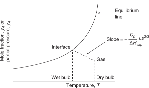
A graph illustrates the humidification process.

Figure 25.2 Representation of a humidification process in terms of an equilibrium curve and operating curve.

Problems of this type are also of importance in a number of related situations, including fog formation in environmental applications. A simple numerical example is presented in Example 25.1 to get an appreciation for the numbers.

Example 25.1 Humidity Calculation from Wet Bulb Temperature

Find the gas composition and relative humidity if the (dry) gas temperature is 31.8 °C and the wet bulb temperature is 26.8 °C. The total pressure is 1.01 bar. The following values of physical properties evaluated at 300 K are used: ρ = 1.1769 kg/m³; c_p = 1006 J/kg.K; ν = 1.57 × 10^–5 m²/s. Pr = 0.713; Le = 0.847.

Solution

The vapor pressure of water at 26.8 °C is computed using the Antoine equation and equal to 26.35 mm Hg. Hence y_s has a value of 26.34/760 or 0.0347. Using Equation 25.5, y_b is determined to be 0.0313.

The results are normally reported in terms of relative humidity, which is defined as follows:

Re l a t i v e h u m i d i t y = \frac{m o l e f r a c t i o n i n a i r}{m o l e f r a c t i o n i f t h e a i r w e r e s a t u r a t e d}

$Re l a t i v e h u m i d i t y = \frac{m o l e f r a c t i o n i n a i r}{m o l e f r a c t i o n i f t h e a i r w e r e s a t u r a t e d}$

In the above example, if the air were saturated at the temperature of 31.8 °C it would exert a vapor pressure of 35.17 mm Hg. Hence the mole fraction would be 35.17/760 or 0.0463 while the actual value is 0.0313. The relative humidity is therefore 0.0313/0.0463 or 67.6%.

In the next section we present an important application of evaporative cooling, which is the principle behind the cooling towers used widely in process industries.

25.2 Humidification: Cooling Towers

Humidification refers to transfer of a liquid phase component (usually water) into a gas stream. Water temperature drops upon evaporation to dry air when the process is operated in an adiabatic manner. This principle can be used to cool large quantities of hot water exiting from heat exchangers in order to recycle the water back to these process units. This cooling process is done is a cooling tower, which finds extensive application in power plants, nuclear reactors, refineries and petrochemical plants. In this section we study the application of heat and mass transfer principles to develop a basic design equation for the cooling tower.

25.2.1 Classification

Depending on how the air is forced through the system, cooling towers can be broadly classified into two types:

Natural draft: This utilizes the buoyancy of warm, moist air compared to the outside dry cooler air. The buoyancy difference causes a density difference, which produces an upward flow of air through the tower. These are suitable for large power plants.
Forced draft: The air flow is induced by a blower or fan. These are more suitable for small capacity systems, such as cooling in air conditioning units.

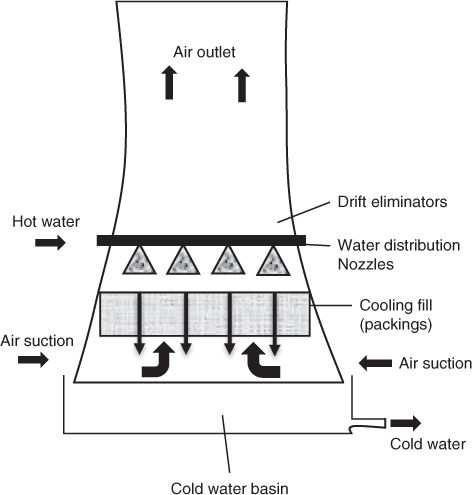
The natural draft cooling tower is usually of hyperboloid design; an illustrative diagram is shown in Figure 25.3. The hyperbolid design is effective from a mechanical strength point of view and also for minimum material cost. It also aids in increasing the upflow velocity of air, thereby improving the gas flow rate.

A diagram of the natural draft cooling tower is shown.

Figure 25.3 Counterflow cooling tower with natural draft.

A second classification is based on the flow pattern of water and air. In the counterflow type, water and air flow countercurrent to each other. The flow patterns in a natural draft cooling tower by design are countercurrent. In the cross-flow type, liquid flows downward but the gas flow is in horizontal direction, that is, perpendicular to liquid flow.

25.2.2 General Design Considerations

The concept of wet and dry bulb temperature was introduced in Section 25.1 and is important in the design of cooling towers. The dry bulb temperature is the actual temperature of the gas at a given water vapor composition (or given humidity) while the wet bulb temperature is the temperature if the gas were saturated with the vapor. If the gas (dry bulb) temperature is the same as the wet bulb temperature, the gas is saturated and no mass transfer from liquid can take place. Hence the local water temperature has to be above the wet bulb temperature of the air in order to have any cooling. If the gas is saturated then there is no cooling.

Usually cooling towers are designed so that the discharge temperature of water is about 3 to 5 °C above the wet bulb temperature corresponding to the inlet gas conditions. This provides an adequate driving force for mass and heat transfer. This temperature difference (outlet water temperature minus the wet bulb temperature of the inlet air) is called the approach. The change in water temperature from inlet to outlet is called the range.

The mass flow ratio ${\dot{m}}_{L} / {\dot{m}}_{G}$ ${\dot{m}}_{L} / {\dot{m}}_{G}$ is an important parameter that affects the performance of the cooling tower. The mass transfer coefficient is normally correlated in terms of the flow ratio parameter. Typical mass velocities of water in cross-flow arrangements are in the range of 1.8 to 2.7 kg/m²s and the superficial air velocity falls in the range of 1.5-4 m/sec (Mills, 1993). The gas and liquid flow rates can be independently varied in this arrangement. However, in a natural circulation type of arrangement they can not be varied independently. The buoyancy producing the air flow is determined by the exit condition of the air leaving the tower. Hence an iterative solution is needed to calculate the air flow rate for this type of arrangement for a given liquid rate and the specified level of cooling.

25.3 Model for Counterflow

Figure 25.3 showed an equipment schematic of a natural draft counterflow cooling tower. Water flows as thin films down a suitable packing while the air flows upwards. The driving force for air flow is caused by the density difference between the moist and the warm air. The governing equations are based on heat and mass balances on a mesoscopic control volume and use the plug flow assumption. The control volume is shown in Figure 25.4.

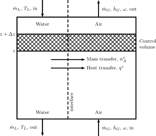
A schematic diagram of a counter flow cooling tower is shown.

Figure 25.4 Schematic of the control volume for the gas and water phase to model a counterflow cooling tower.

25.3.1 Mass Balance Equations

Mass units are commonly used and the driving force for mass transfer is based on the mass fraction difference.

The mass balance for water flow rate is

\begin{matrix} \frac{d {\dot{m}}_{L}}{d z} = A n_{A}^{υ} & (25.6) \end{matrix}

$\begin{matrix} \frac{d {\dot{m}}_{L}}{d z} = A n_{A}^{υ} & (25.6) \end{matrix}$

The mass balance for gas is

\begin{matrix} \frac{d {\dot{m}}_{G}}{d z} = A n_{A}^{υ} & (25.7) \end{matrix}

$\begin{matrix} \frac{d {\dot{m}}_{G}}{d z} = A n_{A}^{υ} & (25.7) \end{matrix}$

In these equations, A is the cross-sectional area and $n_{A}^{υ}$ $n_{A}^{υ}$ is the mass transfer rate of water based on unit volume. The latter is given by the mass transport relation and is equal to

\begin{matrix} n_{A}^{υ} = k_{ω} a_{g l} (ω_{s} - ω) & (25.8) \end{matrix}

$\begin{matrix} n_{A}^{υ} = k_{ω} a_{g l} (ω_{s} - ω) & (25.8) \end{matrix}$

Here k_ω is the intrinsic mass transfer coefficient based on the mass fraction driving force and a_gl is the transfer area per unit tower volume. Note that a low flux model is implied and no drift flux correction is used; these approximations are valid in view of the low water vapor pressures at the operating conditions. ω is the actual mass fraction of water vapor in the gas phase. ω_s is the saturation mass fraction of water corresponding to the interface temperature, and can be calculated as

\begin{matrix} ω_{s} = \frac{18 y_{s}}{18 y_{s} + 29 (1 - y_{s})} & (25.9) \end{matrix}

$\begin{matrix} ω_{s} = \frac{18 y_{s}}{18 y_{s} + 29 (1 - y_{s})} & (25.9) \end{matrix}$

where y_s is the mole fraction of the saturated vapor given as p_vap/p_total. p_vap, the vapor pressure, in turn can be calculated using the Antoine equation corresponding to the liquid temperature.

Water vapor mass balance in the gas phase air completes the set of mass balance equations:

\begin{matrix} \frac{d}{d z} (ω {\dot{m}}_{G}) = A n_{A}^{υ} & (25.10) \end{matrix}

$\begin{matrix} \frac{d}{d z} (ω {\dot{m}}_{G}) = A n_{A}^{υ} & (25.10) \end{matrix}$

The next set of equations are the enthalpy balances for the gas and liquid phases.

25.3.2 Enthalpy Balance Equations

The enthalpy balance for water is written as

\begin{matrix} \frac{d ({\dot{m}}_{L} {\hat{h}}_{L})}{d z} = A Q^{υ} & (25.11) \end{matrix}

$\begin{matrix} \frac{d ({\dot{m}}_{L} {\hat{h}}_{L})}{d z} = A Q^{υ} & (25.11) \end{matrix}$

Q^v is the heat transferred from water to air per unit volume. ĥ_L is defined as the enthalpy of the liquid per unit mass.

The heat balance for air is

\begin{matrix} \frac{d ({\dot{m}}_{G} {\hat{h}}_{G})}{d z} = A Q^{υ} & (25.12) \end{matrix}

$\begin{matrix} \frac{d ({\dot{m}}_{G} {\hat{h}}_{G})}{d z} = A Q^{υ} & (25.12) \end{matrix}$

Here ĥ_G is the specific enthalpy of the gas phase, which is a mixture of air and water vapor.

Transport relation is now needed for Q^v, which are presented later after defining equations for the enthalpies.

Auxiliary Relations for Enthalpy

Additional auxiliary conditions for enthalpy are needed to close the model, which we will discuss next.

A reference temperature and a reference enthalpy have to be chosen in order to calculate the gas phase and liquid phase enthalpies. It is convenient to choose the reference temperature T_ref as zero 0 °C. (All temperature from now on in the model will be in degrees Celsius). Enthalpy of water at 0 °C is taken as the reference enthalpy.

The enthalpy of liquid water at any other temperature then is:

\begin{matrix} {\hat{h}}_{L} = c_{p L} T_{L} & (25.13) \end{matrix}

$\begin{matrix} {\hat{h}}_{L} = c_{p L} T_{L} & (25.13) \end{matrix}$

The enthalpy term in the gas phase in turn is given by the following equation:

\begin{matrix} {\hat{h}}_{G} = {\bar{c}}_{p G} T_{G} + ω {\hat{h}}_{l g} & (25.14) \end{matrix}

$\begin{matrix} {\hat{h}}_{G} = {\bar{c}}_{p G} T_{G} + ω {\hat{h}}_{l g} & (25.14) \end{matrix}$

where ĥ_lg is the latent heat of vaporization for water at 0°C. ${\bar{c}}_{p G}$ ${\bar{c}}_{p G}$ is the specific heat of the mixture, given as

{\bar{c}}_{p G} = (1 - ω) c_{p, a} + ω c_{p, w}

${\bar{c}}_{p G} = (1 - ω) c_{p, a} + ω c_{p, w}$

c_p,w is the specific heat of the water vapor and c_p,a is the specific heat of air.

Hence the enthalpy of the gas phase can be related to the temperature of the gas as follows:

\begin{matrix} {\hat{h}}_{G} = (1 - ω) c_{p}, T_{G}_{a} + ω (c_{p}, T_{G}_{w} + {\hat{h}}_{l g}) & (25.15) \end{matrix}

$\begin{matrix} {\hat{h}}_{G} = (1 - ω) c_{p}, T_{G}_{a} + ω (c_{p}, T_{G}_{w} + {\hat{h}}_{l g}) & (25.15) \end{matrix}$

Rate of Heat Transfer

The rate of heat transfer from the gas–liquid interface to the bulk gas consists of two terms: the convective heat transfer from the interface to the bulk gas due to temperature difference and the enthalpy carried by the flux of water vapor to the gas phase.

Convective heat transfer is given as ha_gl(T_i – T_g). Here h is the heat transfer coefficient from the interface to the bulk gas.

The enthalpy due to mass transfer is equal to $n_{A}^{υ} ({\hat{h}}_{w i})$ $n_{A}^{υ} ({\hat{h}}_{w i})$ . Here ĥ_wi is the enthalpy of the water vapor at the interface conditions.

The temperature difference in the liquid is assumed to be small and the assumption that T_i = T_L is made here. Hence ĥ_wi can be approximated as ĥ_ws, the enthalpy of the water vapor at liquid temperature.

Hence the heat transfer rate Q^v is given as

\begin{matrix} Q^{υ} = n_{A}^{υ} {\hat{h}}_{w s} + h a_{g l} (T_{L} - T_{g}) & (25.16) \end{matrix}

$\begin{matrix} Q^{υ} = n_{A}^{υ} {\hat{h}}_{w s} + h a_{g l} (T_{L} - T_{g}) & (25.16) \end{matrix}$

This completes the model formulation. The complete set of equations contains five primary variables: mass flow rates of water and gas, water vapor mole fraction in the gas, and gas and liquid enthalpies. Three mass balances and two enthalpy balances provide the five equations. In addition there are three auxiliary variables: T_L, T_G, and ω_s. Two enthalpy relations (Equations 25.13 and 25.14) and the vapor–liquid equilibrium relation (Equation 25.9) provide three relations and hence the model set is correctly specified. A complete solution is involved and can be done numerically, but is not normally used for design due to uncertainty in the values of the heat and mass transfer coefficients. A simpler and more practical approach is to combine the model equations into a single equation after making some simplifying assumptions. This is the focus of the next section.

25.3.3 Merkel Equation

The set of equations can be reduced to a single equation for enthalpy as shown in the following analysis. We have many invariants and this permits the number of equations to be reduced. In fact one equation is sufficient to calculate the performance of the cooling tower. This equation, derived in 1925, is called the Merkel equation. The derivation leading to this equation is presented in the following section.

We start with the gas phase enthalpy balance given by Equation 25.6 and expand the derivative on the left-hand side:

\begin{matrix} {\dot{m}}_{G} \frac{d {\hat{h}}_{G}}{d z} + {\hat{h}}_{G} \frac{d {\dot{m}}_{G}}{d z} = A Q^{υ} & (25.17) \end{matrix}

$\begin{matrix} {\dot{m}}_{G} \frac{d {\hat{h}}_{G}}{d z} + {\hat{h}}_{G} \frac{d {\dot{m}}_{G}}{d z} = A Q^{υ} & (25.17) \end{matrix}$

Further, from Equation 25.7 we have

\frac{d {\dot{m}}_{G}}{d z} = A n_{A}^{υ}

$\frac{d {\dot{m}}_{G}}{d z} = A n_{A}^{υ}$

Using this in the second term on the left-hand side, the previous equation is changed to

\begin{matrix} {\dot{m}}_{G} \frac{d {\hat{h}}_{G}}{d z} + A n_{A}^{υ} {\hat{h}}_{G} = A Q^{υ} & (25.18) \end{matrix}

$\begin{matrix} {\dot{m}}_{G} \frac{d {\hat{h}}_{G}}{d z} + A n_{A}^{υ} {\hat{h}}_{G} = A Q^{υ} & (25.18) \end{matrix}$

Using Equation 25.16 for Q_v and moving the $n_{A}^{υ}$ $n_{A}^{υ}$ term to the right-hand side gives

\begin{matrix} {\dot{m}}_{G} \frac{d {\hat{h}}_{G}}{d z} = A n_{A}^{υ} (h_{w s} - h_{G}) + A h a_{g l} (T_{L} - T_{g}) & (25.19) \end{matrix}

$\begin{matrix} {\dot{m}}_{G} \frac{d {\hat{h}}_{G}}{d z} = A n_{A}^{υ} (h_{w s} - h_{G}) + A h a_{g l} (T_{L} - T_{g}) & (25.19) \end{matrix}$

The heat transfer coefficient h is taken as $k_{ω} {\bar{c}}_{p, G}$ $k_{ω} {\bar{c}}_{p, G}$ , which is an analogy useful for a Lewis number of one. This is the first assumption in the Merkel approach. Hence the previous equation simplifies to

\begin{matrix} {\dot{m}}_{G} \frac{d {\hat{h}}_{G}}{d z} = A k_{ω} a_{g l} [(ω_{s} - ω) ({\hat{h}}_{w s} - {\hat{h}}_{G}) + {\bar{c}}_{p, G} (T_{L} - T_{g})] & (25.20) \end{matrix}

$\begin{matrix} {\dot{m}}_{G} \frac{d {\hat{h}}_{G}}{d z} = A k_{ω} a_{g l} [(ω_{s} - ω) ({\hat{h}}_{w s} - {\hat{h}}_{G}) + {\bar{c}}_{p, G} (T_{L} - T_{g})] & (25.20) \end{matrix}$

An analysis of the magnitude of the various terms in the above equation indicates that it can be simplified to

\begin{matrix} {\dot{m}}_{G} \frac{d {\hat{h}}_{G}}{d z} = A k_{ω} a_{g l} ({\hat{h}}_{s} - {\hat{h}}_{G}) & (25.21) \end{matrix}

$\begin{matrix} {\dot{m}}_{G} \frac{d {\hat{h}}_{G}}{d z} = A k_{ω} a_{g l} ({\hat{h}}_{s} - {\hat{h}}_{G}) & (25.21) \end{matrix}$

Here ĥ_s = enthalpy of saturated gas at water temperature (the equation for this is given later as 25.25) and ĥ_G = enthalpy of gas at gas temperature. This is given by Equation 25.14.

A similar manipulation for the liquid gives

\begin{matrix} {\dot{m}}_{L} \frac{d {\hat{h}}_{L}}{d z} = A κ_{ω} a_{g l} ({\hat{h}}_{s} - {\hat{h}}_{G}) & (25.22) \end{matrix}

$\begin{matrix} {\dot{m}}_{L} \frac{d {\hat{h}}_{L}}{d z} = A κ_{ω} a_{g l} ({\hat{h}}_{s} - {\hat{h}}_{G}) & (25.22) \end{matrix}$

The assumption that the evaporation rate is small and therefore the water flow rate remains constant is used in arriving at this result; this is the second assumption in the Merkel method. Using ${\hat{h}}_{L} = c_{p L} d T_{L}$ ${\hat{h}}_{L} = c_{p L} d T_{L}$ the previous equation can be represented as

\begin{matrix} {\dot{m}}_{L} c_{p L} \frac{d T l}{d z} = A k_{ω} a_{g l} ({\hat{h}}_{s} - {\hat{h}}_{G}) & (25.23) \end{matrix}

$\begin{matrix} {\dot{m}}_{L} c_{p L} \frac{d T l}{d z} = A k_{ω} a_{g l} ({\hat{h}}_{s} - {\hat{h}}_{G}) & (25.23) \end{matrix}$

The integrated form of this is called the Merkel equation; it provides the liquid temperature distribution and the exit water temperature in the tower.

The enthalpy of the gas at the gas temperature is needed in the integration of Equation 25.23. This is not easy to use since it requires the simultaneous calculation of the mole fraction of water vapor in the gas. However, the enthalpy of the gas need not be calculated from this equation, but can be related to the liquid temperature as shown below. This is yet another computational simplification.

An overall heat balance between any cross-section at z and the bottom of the tower gives

{\hat{h}}_{G} = {\hat{h}}_{G, i n} + \frac{{\dot{m}}_{L}}{{\dot{m}}_{G}} ({\hat{h}}_{L} - {\hat{h}}_{L, o u t})

${\hat{h}}_{G} = {\hat{h}}_{G, i n} + \frac{{\dot{m}}_{L}}{{\dot{m}}_{G}} ({\hat{h}}_{L} - {\hat{h}}_{L, o u t})$

or equivalently in terms of the liquid temperature

\begin{matrix} {\hat{h}}_{G} = {\hat{h}}_{G, i n} + \frac{{\dot{m}}_{L}}{{\dot{m}}_{G}} c_{p L} (T_{L} - T_{L, o u t}) & (25.24) \end{matrix}

$\begin{matrix} {\hat{h}}_{G} = {\hat{h}}_{G, i n} + \frac{{\dot{m}}_{L}}{{\dot{m}}_{G}} c_{p L} (T_{L} - T_{L, o u t}) & (25.24) \end{matrix}$

Hence the ĥ_G can be calculated at any given T_L and used in Equation 25.24.

The h_s is based on saturation conditions at water temperature and can be calculated from the following equation:

\begin{matrix} {\hat{h}}_{s} = (1 - ω_{s}) c_{p}, T_{L}_{a} + ω_{s} c_{p}, T_{L}_{w} + {\hat{h}}_{l g} ω_{s} & (25.25) \end{matrix}

$\begin{matrix} {\hat{h}}_{s} = (1 - ω_{s}) c_{p}, T_{L}_{a} + ω_{s} c_{p}, T_{L}_{w} + {\hat{h}}_{l g} ω_{s} & (25.25) \end{matrix}$

The vapor pressure data is needed to find ω_s at a given value of T_L, which can be calculated from Equation 25.9 with the help of the Antoine equation for vapor pressure. Thus all the quantities needed in the Merkel equation are known.

The Merkel equation is often arranged into an HTU (height of a transfer unit) and NTU (number of transfer units) form similar to that for gas absorption. Thus the height of the tower is calculated as

H = HTU × NTU

where HTU is defined as

H T U = \frac{{\dot{m}}_{L} c_{p L}}{A κ_{ω} a_{g l}}

$H T U = \frac{{\dot{m}}_{L} c_{p L}}{A κ_{ω} a_{g l}}$

and NTU is defined as

N T U = \int_{T_{L, o u t}}^{T_{L, i n}} \frac{d T_{L}}{{\hat{h}}_{s} - {\hat{h}}_{G}}

$N T U = \int_{T_{L, o u t}}^{T_{L, i n}} \frac{d T_{L}}{{\hat{h}}_{s} - {\hat{h}}_{G}}$

Example 25.2 provides an illustration of the calculation of the NTU parameter.

Example 25.2 NTU Calculation for a Cooling Tower

A cooling tower is to be designed to cool water from 40 °C to 26 °C. The inlet air is at 10 °C and saturated. A liquid to air mass flow ratio of one is used. Calculate the number of transfer units needed.

Solution

The data needed for the various enthalpy calculations are as follows: c_p,w = 1864 J/kg K, c_p,a = 1005 J/kg K, and ĥ_lg = 2.5 × 10⁶ J/kg.

The saturation vapor pressure for any given temperature can be calculated using the Antoine equation:

\log_{10} p_{s a t} (mm Hg) = A - \frac{B}{T + C}

$\log_{10} p_{s a t} (mm Hg) = A - \frac{B}{T + C}$

and the constants for water are as follows: A = 8.07131, B = 1730.63, C = 233.246, and T is in °C.

The mole fraction y_s at saturation is p_sat/760, assuming a total pressure of 760 mm Hg. The mass fraction at saturation ω_s is then calculated using Equation 25.9.

This information is used to calculate the saturation enthalpy and enthalpy of the gas at several values of the liquid temperature between 26 °C and 40 °C. The saturation enthalpy is calculated using Equation 25.25 in the text.

The gas enthalpy is calculated using Equation 25.24. For this we need to calculate the value of ĥ_G,in. The inlet air vapor mass fraction is known since it is assumed to be saturated. Hence Equation 25.15 can be used to find the inlet air enthalpy. The value is 29 kJ/kg; you should verify the calculation.

The results for ĥ_s and ĥ_g at some selected liquid temperatures are as follows:

T_L,C	*ĥ_s*, kJ/kg	ĥ_G kJ/kg
26	79	29
33	112	58
40	158	87

The NTU can be found by the area under the curve of 1/(ĥ_s – ĥ_G) versus T_L or by using the Simpson rule after generating a table similar to the above in the temperature interval from the exit to the inlet. The value obtained using the Simpson rule is 1.06. It is easy to set up an Excel spreadsheet or a MATLAB m-file to do these calculations.

25.4 Cross-Flow Cooling Towers

In a cross-flow arrangement, the air and water flow in cross direction. The schematic is shown in Figure 25.5. A cross-flow arrangement is more suitable for small capacity plants.

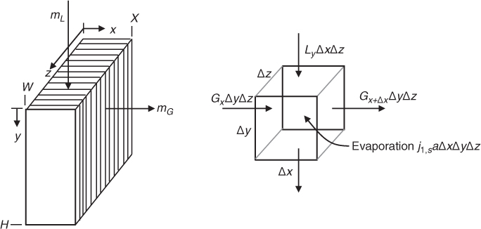
A schematic diagram of a cross-flow cooling tower is shown.

Figure 25.5 Schematic of a cross-flow cooling tower. Adapted from Mills, Heat and Mass Transfer. Erwin Publications, page 1105.

The balance equations (using Merkel assumptions similar to that in counterflow) lead to the following equations for predicting the performance of this equipment. For gas enthalpy, which varies in the x-direction, we get

\begin{matrix} \frac{\partial {\hat{h}}_{G}}{\partial x} = \frac{k_{ω} a_{g l}}{G} ({\hat{h}}_{s} - {\hat{h}}_{G}) & (25.26) \end{matrix}

$\begin{matrix} \frac{\partial {\hat{h}}_{G}}{\partial x} = \frac{k_{ω} a_{g l}}{G} ({\hat{h}}_{s} - {\hat{h}}_{G}) & (25.26) \end{matrix}$

G is the superficial mass velocity of the gas, equal to ${\dot{m}}_{G} / H W$ ${\dot{m}}_{G} / H W$ .

For liquid enthalpy, which varies in the y-direction (marked vertically downward) we have

\begin{matrix} \frac{\partial {\hat{h}}_{L}}{\partial y} = - \frac{k_{y} ω a_{g l}}{L} ({\hat{h}}_{s} - {\hat{h}}_{G}) & (25.27) \end{matrix}

$\begin{matrix} \frac{\partial {\hat{h}}_{L}}{\partial y} = - \frac{k_{y} ω a_{g l}}{L} ({\hat{h}}_{s} - {\hat{h}}_{G}) & (25.27) \end{matrix}$

L is the superficial liquid velocity, ${\dot{m}}_{L} / (W X)$ ${\dot{m}}_{L} / (W X)$ .

The liquid enthalpy equation is commonly expressed in terms of liquid temperature as

\begin{matrix} c_{p L} \frac{\partial T_{L}}{\partial y} = - \frac{k_{ω} a_{g l}}{L} ({\hat{h}}_{s} - {\hat{h}}_{G}) & (25.28) \end{matrix}

$\begin{matrix} c_{p L} \frac{\partial T_{L}}{\partial y} = - \frac{k_{ω} a_{g l}}{L} ({\hat{h}}_{s} - {\hat{h}}_{G}) & (25.28) \end{matrix}$

The required boundary conditions are

At x = 0, the gas entrance, ĥ_G = ĥ_G,in
At y = 0, the liquid, ĥ_L = ĥ_L,in or T_L = T_L,i.

The balance equations are a pair of first-order partial differential equations now. These require a numerical solution. For example, a suitable finite difference approximation can be set up for the derivatives and the set of algebraic equations can be set up at each mesh point. The equations can be solved in a sequential manner starting at the top row.

Suppose the system is discretized into meshes in the x- and y-directions. See Figure 25.6, which shows an N X M discretization.

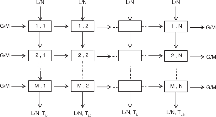
A diagram showing the simulation process of the cross-flow cooling tower.

Figure 25.6 A cell-by-cell approach to simulate the cross-flow cooling tower.

The mesh size in the x-direction is W/N and the mesh size in the y-direction is H/M. Each mesh defines a cell, which are marked and numbered in the figure. The entrance conditions for both the gas and the liquid are known at the top corner cell (1,1) on the left of the figure. The conditions on the liquid side are known for all the cells in the top row. Hence starting from cell (1,1) we can successively solve the equation for this entire row for the gas enthalpy values and the liquid exit temperature values from this row. The calculated exit liquid conditions for this row are used as the inlet conditions for the next row. For the gas, the conditions at the entrance of the inlet cell (2,1 now) are known. Hence we can sweep across row 2 to complete the solution for this row. This provides all the data required for row 3, and so on.

The liquid exit from the last row is finally calculated for all the cells in that row. An average value is then calculated and this will represent the liquid exit temperature.

The gas and liquid flows entering each cell are assumed to be constant. This applies since the extent of liquid evaporated in a cooling tower is usually small. Note that this was also the assumption used in the Merkel model in the previous section. The gas mass velocity in each cell is to be taken as G/M, where G is the total gas velocity. Similarly the liquid velocity in each cell is L/N. The computational implementation is not shown here and is left as an exercise problem.

25.5 Drying

Drying, as the name implies, refers to the process of removal of moisture (or other liquid) content of a solid by heating or by contacting with a hot gas. It is often the final step of a series of operations and the dried solid is usually ready for final packaging. Examples include crystalline salts to produce a free flowing material, food to prevent spoilage, detergent, pharmaceutical capsules, wood, soap, paper, and many other products.

25.5.1 Types of Dryers

One classification is based on whether the solid is in direct contact with hot gas or is heated indirectly from a hot metal surface. The first type are also called adiabatic or direct dryers while the second type are known as indirect or nonadiabatic dryers. Drying can also be done by radiation heat transfer or microwave energy.

Dryers may also be classified into two types: batch dryers where the solid is stagnant and continuous dryers where the solid is moving in the dryer.

Batch dryers with stagnant solids are generally tray dryers where the solid to be dried is kept in a tray with a suitable arrangement for the flow of the hot drying gas. The gas flow pattern can be either parallel flow or cross-flow. A batch dryer with a moving solid is the fluidized bed dryer, where the solids are separated from each other and kept suspended in motion by the gas. The rotary dryer is another arrangement where the solids are in motion.

A continuous dryer is the flash dryer, where the solids are transported by the gas. Fluid bed dryers can also be operated in a continuous manner. Spray dryers are another type and suitable when the solid to be dried is presented as a dilute solution in a liquid. The various types of dryers are shown in Figure 25.7.

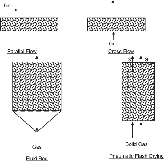
A set of four diagrams showing the common types of adiabatic dryers.

Figure 25.7 Common types of adiabatic dryers (direct heat dryers) and the contacting pattern of gas and solid.

Dryers are seldom designed by the user and usually bought from specialized equipment dealers. Nevertheless the analysis of drying represents an elegant example of simultaneous heat and mass transfer and also illuminates the different models for moisture transport in porous media (which has applications in other fields as well, for example, groundwater transport, flow in porous beds. and so on). Hence it is useful to study the basic mechanism of drying and examine how it relates to mass transfer theory. This is the focus of the rest of this chapter.

25.5.2 Types of Solids

Solids being dried are generally of two types:

Category 1: Granular or crystalline solids where the moisture is in the open pores between particles. For these type of materials, the structure of the solid is not changed by the moisture removal.
Category 2: Amorphous, fibrous, or gel type of solids: These are materials such as vegetables, wood, soap, and so on. Moisture is held mostly in the interior of the solid. Solid properties change with drying and considerable shrinkage can occur.

Solids may also be classified as hygroscopic or non-hygroscopic. The former contains both unbound (moisture held on the surface) and bound moisture (held chemically with the solid). Non-hygroscopic materials have only unbound moisture. The classification is important in interpretation of the drying rate and the phenomena of drying of these materials.

Moisture content denoted as X is commonly expressed as mass of moisture per gm of bone dry solid. This is same as mass fraction on a dry basis and is convenient since the mass of dry solid remains constant through the drying process. Mass percent is also used in many papers.

25.5.3 Constant and Falling Rates

Consider a porous solid that is being dried in presence of hot air. The process is again one of simultaneous heat and mass transfer. Heat is transferred to the solid and moisture is removed from the solid. An illustrative plot of moisture content of the solid as a function of time is shown in Figure 25.8. The region A to B is the preheating period where the solid is heated to the wet bulb temperature of the gas. No appreciable loss of moisture takes place during this time.

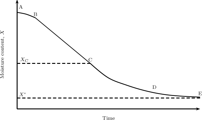
A line graph to plot the moisture content of the solid, for time.

Figure 25.8 Illustrative plot of moisture content versus time showing various regions for drying. AB = initial heating period, BC = constant rate period, CD = falling rate period, DE = second falling rate period.

After this the solid temperature remains constant for a while at the wet bulb temperature and the moisture content decreases as a linear function of time (BC). This is called the constant rate period. The constant rate period lasts until a critical moisture content (marked as C in the figure) is reached. At this point dry patches appear on the solid and after this period, the rate of drying starts to fall. This is referred to as the falling rate period. The rate decreases even further after point D is reached. This is called the second falling rate period while region CD is called the first falling rate period. The final moisture content after a long period of time is referred to as the equilibrium moisture content. Some solids may exhibit only one falling rate period.

Results of this nature were generated by Professor Sherwood as early as 1929. If the X versus t curve is differentiated with time we get the rate of drying; this is more illustrative of the four periods described earlier (see Figure 25.9).

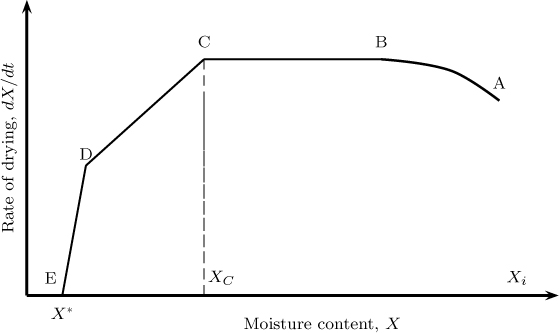
Figure 25.9 Illustrative plot of rate of drying as a function of the moisture content. C = critical moisture content; E = equilibrium moisture content.

The mechanism and models to calculate the rate for these periods will now be discussed.

25.6 Constant Rate Period

The transport of heat and mass in the gas film surrounding the solid determines the rate of drying. In the constant rate period, the internal diffusion or capillary flow is fast enough to maintain a constant surface concentration. The surface of the solid is assumed to be wetted and covered by a liquid film and external transport in the boundary layer near the surface is assumed to be the rate controlling step (see Figure 25.10).

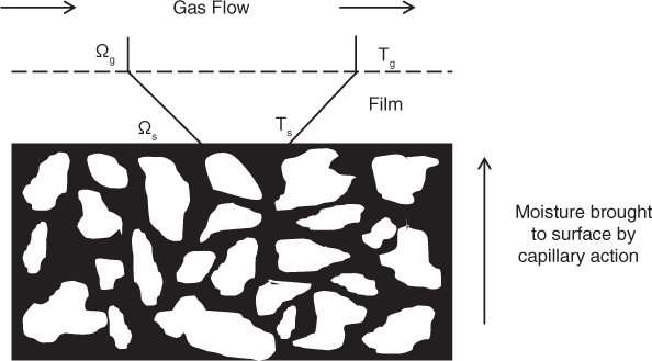
An illustration depicts the constant rate period.

Figure 25.10 Mechanism and rate of transport in the constant rate period. Moisture is available at the surface due to rapid internal transport and the process is limited by the rate of external mass or heat transfer.

The rate of drying can be predicted by either mass transfer considerations or heat transfer considerations. The following equations apply respectively:

\begin{matrix} \dot{m} = κ_{ω} A (ω_{s} - ω_{g}) F & (25.29) \end{matrix}

$\begin{matrix} \dot{m} = κ_{ω} A (ω_{s} - ω_{g}) F & (25.29) \end{matrix}$

\begin{matrix} \dot{m} = \frac{h A (T_{g} - T_{s})}{{\hat{h}}_{l g}} & (25.30) \end{matrix}

$\begin{matrix} \dot{m} = \frac{h A (T_{g} - T_{s})}{{\hat{h}}_{l g}} & (25.30) \end{matrix}$

Either of the equations can be used to predict the drying rate. In one case we need to know the mass transfer coefficient from the surface to the bulk gas while in the other the heat transfer coefficient from the bulk gas to the solid surface is required. The equation from heat transfer considerations is more commonly used since the heat transfer data are usually more accurate than that for the mass transfer coefficient. The heat transfer coefficient (for parallel to the solid) is in turn usually calculated using the Mujumdar (1995) correlation:

Nu = 0.037Re^0.8 Pr^1/3

where Nu and Re are defined using L_ref = L, the length of gas flow over the surface. This correlation is similar to the Dittus-Boelter correlation with the leading coefficient somewhat higher. Seader et al. (2011) presented a simplified version for flow parallel to the solid:

h = 0.0204G^0.8

Here G is kg/m²hr and h is the traditional SI unit of W/m²K.

Another arrangement is packed beds with through circulation of the gas. The following correlation is suggested by Mujumdar (1995) and also by Seader et al. (2011):

h = 0.151 G^{0.59} / d_{p}^{0.41} for Re \geq 350

$h = 0.151 G^{0.59} / d_{p}^{0.41} for Re \geq 350$

and

h = 0.214 G^{0.49} / d_{p}^{0.5} for Re < 350

$h = 0.214 G^{0.49} / d_{p}^{0.5} for Re < 350$

The Reynolds number is defined in the usual manner for packed beds as d_pG/μ. The units are kg/m²hr for G and meter for d_p.

Correlations are available for various other dryer arrangements (e.g., fluidized beds, spouted beds, etc.) and a compact tabular summary is available in Table 18.6 Seader et al. (2011) and can be used for first-level design calculations.

It is common to use the rate of drying parameter dX/dt. For the constant rate period, this is a constant equal to R_c, which is related to ${\dot{M}}_{A}$ ${\dot{M}}_{A}$ as follows:

R_{c} = \dot{m} A / m_{s}

$R_{c} = \dot{m} A / m_{s}$

where m_s is the mass of bone dry solid. The change in moisture constant of the solid can then be calculated using the rate of drying:

\begin{matrix} \frac{d X}{d t} = - R_{c} & (25.31) \end{matrix}

$\begin{matrix} \frac{d X}{d t} = - R_{c} & (25.31) \end{matrix}$

This gives

X = X₀ – R_ct for t < t_c

where X₀ is the initial moisture content. (The drop in the initial moisture during the preheating period, AB, is ignored here.)

The constant rate applies until a critical moisture content, X_c, is reached. This critical value is difficult to predict and depends on many parameters including the thickness of the solid, initial porosity, the extent of shrinkage, and pore size changes during drying. There is discussion on the prediction of this parameter is later in this chapter.

The falling rate starts at X = X_c and hence the time at which the falling rate starts is

\begin{matrix} t_{c} = \frac{X_{0} - X_{c}}{R_{C}} & (25.32) \end{matrix}

$\begin{matrix} t_{c} = \frac{X_{0} - X_{c}}{R_{C}} & (25.32) \end{matrix}$

25.7 Falling Rate Period

Falling rate is caused by lack of moisture at the surface due to the formation of a patch of dry solid at the gas–solid surface. The thickness of the dry patch increases with time and moves inward to the solid. The rate of drying is now determined by the rate of heat and mass transport in this region. The governing equations are transient mass and heat transport in the dry region together with external transport in the boundary layer. An illustration of the situation and mechanism in the falling rate period is shown in Figure 25.11.

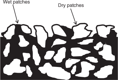
An illustration depicts the first falling rate period.

Figure 25.11 Phenomenological representation of the first falling rate period. The internal transport rate is low and not able to keep up with the evaporation rate; this results in dry patches on the surface.

With further drying, a completely moisture-free region develops near the surface of the solid; this leads to the second falling rate period shown in Figure 25.12.

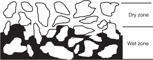
An illustration depicts the second falling rate.

Figure 25.12 Phenomenological representation of the second falling rate period. A dry region and a wet region develop in the solid; the thickness of the dry region increases with time.

The method of calculation for the falling rate period depends on whether the solid is porous or non-porous. The moisture diffusion in the solid is now modeled by a diffusion type of equation for porous category 2 solids. If it is non-porous (categroy 1 granular solid) a capillary transport model is used. Some details on these two types of models are provided in later sections.

However, often simple rate models are used, similar to those used in the power-law kinetics of reaction. These types of models are sometimes referred to as empirical models since they do not attempt to consider any physics of the drying into the model. They are more of a fitting type of model but nevertheless quite useful in practical applications.

25.7.1 Empirical Models

A commonly used model for the rate of drying in the falling rate period states that the rate of drying is proportional to the moisture content. Hence the change in moisture content is given as

\begin{matrix} \frac{d X}{d t} = - k_{d} X & (25.33) \end{matrix}

$\begin{matrix} \frac{d X}{d t} = - k_{d} X & (25.33) \end{matrix}$

k_d is defined as the rate constant for the falling rate period.

The falling rate starts at t = t_c and at this time the moisture content is equal to the critical moisture content X_C. This provides the initial conditions for the previous equation; the integrated form of the rate equation is

\begin{matrix} X = X_{c} \exp [- k_{d} (t - t_{c})] & (25.34) \end{matrix}

$\begin{matrix} X = X_{c} \exp [- k_{d} (t - t_{c})] & (25.34) \end{matrix}$

This describes the moisture content in the falling rate period. This is coupled to the initial period where the rate of drying is constant. Combining the two periods and rearranging the equations, the time to reach a specified final content of X_f is therefore

t_{f} = \frac{X_{0} - X_{c}}{R_{C}} + \frac{1}{k_{d}} \ln (\frac{X_{c}}{X_{f}})

$t_{f} = \frac{X_{0} - X_{c}}{R_{C}} + \frac{1}{k_{d}} \ln (\frac{X_{c}}{X_{f}})$

If the rate constants k_d and R_C are available the equation can be used for estimation of the time needed for drying. Alternatively, the rate constant can be estimated from the measured data and used to model dryer performance for other conditions. Note that R_C can be related to heat transfer coefficient. However, k_d is an empirical parameter in this model and is not correlated to any transport models.

Other rate models are also used. For example a combination of a first-order and second-order model is used in many studies (see, for example, Seader et al., 2011):

\begin{matrix} - \frac{d X}{d t} = k_{d 1} X + k_{d 2} X^{2} & (25.35) \end{matrix}

$\begin{matrix} - \frac{d X}{d t} = k_{d 1} X + k_{d 2} X^{2} & (25.35) \end{matrix}$

This model needs two rate constants, k_d₁ and k_d₂, and is useful for cases where there are two distinct falling rate periods. In the first falling period a linear model with a first-order rate constant is used while the second falling rate period where a combination of first- and second-order rate constants is used. The X versus t behavior of this model essentially involves integration of the dX/dt equation. The integration is done in two parts now corresponding to the two falling rate periods.

25.7.2 Diffusion Type of Models

In the diffusion model, the rate of drying is modeled as a pore diffusion limited process in the solid. In particular, such models are suitable for relatively non-porous solids. For such solids, most of the moisture is in the microvoids inside the solid matrix and a concentration profile is calculated by a transient diffusion model. This type of model was introduced in the drying field by Professor Sherwood himself in 1929 and has found wide applications in the drying of food and pharmaceutical products.

The model equations use the transient diffusion model shown in Chapter 8:

\frac{\partial X}{\partial t} = D \frac{\partial^{2} X}{\partial z^{2}}

$\frac{\partial X}{\partial t} = D \frac{\partial^{2} X}{\partial z^{2}}$

No flux condition is used at z = 0, the impermeable bottom of the cake or the midplane if drying is taking place from both sides.

The boundary condition at the surface, x = L, depends on whether there is a constant rate period or not. If there is no constant rate period, a Dirichlet condition is used, as discussed next.

Dirichlet Problem

Many solids of category 2 do not have significant constant rate period. The surface moisture attains the equilbrium value of X* very quickly for such solids. Hence the Dirichlet condition, X = X*, for the equilibrium moisture content is used as the boundary condition at x = L if there is no constant rate period. This is reasonable for many category 2 type of solids where most of the moisture is held internally. Alternatively t = 0 can be taken as the start of the falling rate period. The internal distribution of moisture during the constant rate period is often ignored and a constant initial condition of X = X₀, the initial moisture content, is often used. With these conditions, the solution for transient diffusion in Section 8.2 can be readily adapted. The moisture distribution as a function of z and t is similar to Equation 8.10.

Average Moisture Content

The average moisture content at any particular time is of interest. This is given by adaptation of the equation shown in Chapter 8:

\begin{matrix} \frac{〈 X 〉 - X^{*}}{X_{0} - X^{*}} = A_{1} B_{1} \exp (- λ^{2} τ) & (25.36) \end{matrix}

$\begin{matrix} \frac{〈 X 〉 - X^{*}}{X_{0} - X^{*}} = A_{1} B_{1} \exp (- λ^{2} τ) & (25.36) \end{matrix}$

A one-term approximation is shown, which is reasonable except for very short times, say τ > 0.1. Using the values of A₁, B₁, and λ₁ from Chapter 8, the drying rate is represented as

\begin{matrix} \frac{〈 X 〉 - X^{*}}{X_{0} - X^{*}} = 0.8106 \exp (- 2.4674 D t / L^{2}) & (25.37) \end{matrix}

$\begin{matrix} \frac{〈 X 〉 - X^{*}}{X_{0} - X^{*}} = 0.8106 \exp (- 2.4674 D t / L^{2}) & (25.37) \end{matrix}$

The data can be fitted to the above equation to find the diffusion coefficient. Then the value of D can be used to find the drying rate for other conditions. The model assumes a constant diffusion coefficient throughout the period of drying, which may not be valid in many situations as indicated by Sherwood. This change can be caused by shrinkage, case hardening, and many other factors. If the diffusion coefficient varies with time a numerical solution is called for.

Initial Period: Neumann Problem

A constant rate period is often observed for a category 1 solid and even for category 2 in many cases. The explanation for the latter case is that there is a surface film of liquid for which the evaporation is controlled by gas phase mass transfer. The boundary condition at the surface is now modified to a constant flux (Neumann type) condition:

\begin{matrix} - D (\frac{d X}{d z})_{z = L} = R_{C} L & (25.38) \end{matrix}

$\begin{matrix} - D (\frac{d X}{d z})_{z = L} = R_{C} L & (25.38) \end{matrix}$

where R_C is the rate of drying in the constant rate period. An analytical solution to the Neumann problem can be derived and follows the method used for heat transfer with constant flux at the surface:

X (ξ, τ) = X_{0} - \frac{R_{C} L}{D} {\frac{ξ^{2}}{2} - \frac{1}{6} + τ - \frac{2}{π^{2}} \sum_{m = 1}^{\infty} \frac{(- 1)^{m}}{m^{2}} \exp (- λ^{2} τ) \cos (λ ξ)}

$X (ξ, τ) = X_{0} - \frac{R_{C} L}{D} {\frac{ξ^{2}}{2} - \frac{1}{6} + τ - \frac{2}{π^{2}} \sum_{m = 1}^{\infty} \frac{(- 1)^{m}}{m^{2}} \exp (- λ^{2} τ) \cos (λ ξ)}$

where the dimensionless parameters are standard as in Chapter 8 for the transient diffusion problem. These are defined as ξ = z/L and τ = Dt/L². The eigenvalue for the Neumann problem is λ_m = mπ. The series part of the solution is important only at the start and may be ignored for τ > 0.1.

The constant rate period ends when the surface moisture reaches the equilibrium value. Hence the model provides a method to find the critical moisture content. Empirical models on the other hand need experimental data for this parameter. Thus the time at which the initial rate ends is found by

τ = \frac{1}{3} + \frac{X_{0} - X^{*}}{R_{C} L / D}

$τ = \frac{1}{3} + \frac{X_{0} - X^{*}}{R_{C} L / D}$

The corresponding average moisture content can be calculated from the Neumann solution and is representative of X_c, the critical moisture content.

The model solution is further continued to find the time to dry the solid all the way to the equilibrium value. The surface boundary condition is now switched to the Dirichlet condition with a value of X* at z = L. A parabolic profile for the moisture would have developed inside the slab during the initial rate period. This is used as the initial condition for the solution in the falling rate period.

A solver like PDEPE is useful for simulation and the two periods can be solved in a sequential manner. One can start off with the Neumann boundary condition to simulate the initial rate period. Once the surface moisture value reaches X*, one switches the boundary condition to Dirichlet with this value and continues the simulation for the falling rate period. The time at which this happens is the end of the constant rate period. The internal moisture content at this time (usually a parabolic profile) is already available as part of the simulation and is automatically used as the initial condition for the falling rate period.

Often the diffusion coefficient is not a constant and changes as a function of the moisture content. Such cases are best handled numerically, for example, using the PDEPE solver.

25.7.3 Capillary Flow Models

The capillary flow model is useful when moisture is present as free moisture in the interstices of the particles rather than in the interior pores of the solid. The capillary model assumes a bed of non-porous spheres surrounding a pore space. Hence it is suitable for granular solids (category 1). Here the liquid is assumed to move by capillary action similar to a wick in a candle. The local variation liquid holdup is assumed to drive the flow of the liquid to the surface. Thus the flow is defined as

j_{L} = - K_{L} ρ_{L} \frac{d ε_{L}}{d z}

$j_{L} = - K_{L} ρ_{L} \frac{d ε_{L}}{d z}$

where K_L is an effective mass conductivity in the porous media. Similarly the vapor flux is modeled as

j_{V} = - D_{V} (ε_{G} - ε_{L}) \frac{d ρ_{G}}{d z}

$j_{V} = - D_{V} (ε_{G} - ε_{L}) \frac{d ρ_{G}}{d z}$

where ρ_G is the vapor density in the gas phase. These “transport models” are then coupled to the conservation model, leading to two equations: one for the liquid holdup profile and the second for the vapor concentration profile in the solid. Details of the model are presented in Chen and Pei (1989). These authors also distinguished two falling rate periods separately and developed models for each case.

25.7.4 Choosing a Model

Whether the diffusion or the capillary model should be used depends on the nature of the solid. Perry and Green (2007) give the following guidelines.

The diffusion model is useful for single-phase solid systems such as gelatin, soap, and glue. It is useful for other solids such as wood and can also be used in the later stages of drying of materials such as textiles, paper, and so on.

The capillary model is useful for coarse grain solids such as sand, paint, and pigments. In view of the complex transport mechanism associated with capillary flow, it is more common to use diffusion models with a fitted value of the effective diffusivity even for these cases.

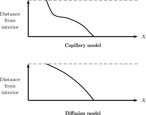
The internal moisture profiles are different for these two types of models. Capillary flow is associated with an internal moisture profile showing a double curvature and a point of inflection. The diffusion model is associated with a smooth curve. The differences in the two models are shown in Figure 25.13. The measurement of the internal moisture profile at various stages of drying may provide some information on which type of model is more suitable.

Two graph shows Profiles of internal moisture content for two types of models.

Figure 25.13 Profiles of internal moisture content for two types of models.

Summary

Humidification and drying are two important processes where the analysis of simultaneous heat and mass transfer considerations are needed. Humidification refers to transfer of moisture from a liquid to an inert gas such as air. Drying refers to transfer of moisture from a wet solid to air.
A liquid exposed to a gas containing an unsaturated vapor will reach a lower temperature than the gas due to evaporative cooling. This phenomena can be used to cool large volumes of liquid and finds application in cooling towers. Large-scale industrial applications are found in power plants. Countercurrent flow and cross-flow are the two common types of operation.
Models for cooling towers are developed using the mass and energy balances together with transport equations for heat and mass. Design models are based on a simplified version of these equations and the Merkel equation is commonly used for design.
The difference between the enthalpy of a saturated gas at liquid temperature and the actual enthalpy of the gas at the gas temperature is taken as the driving force in the Merkel equation. The heat balance in the liquid can then be modeled using this driving force multiplied by a mass transfer coefficient. The integrated form of the enthalpy difference can be expressed in terms of a NTU parameter. The transport coefficient part of the model is usually recast into a HTU parameter and the data for this parameter is available for a number of internal designs of the cooling tower. The height of the packed part of the tower is then the product of the HTU and NTU, a similar concept to that used for absorption columns.
The model for cross-flow design follows an approach similar to counterflow and usually the Merkel equation is used. However, due to the change in flow directions, the resulting equations are a set of partial differential equations for the temperature of the liquid in the downward direction and the enthalpy of the gas in the flow direction. This set of equations can be solved by a finite difference mesh.
Drying, as the name implies, refers to the process of removal of moisture (or other liquid) content of a solid by heating or by contacting with a hot gas. It is often the final step of a series of operations and the dried solid is usually ready for final packaging. Direct contact and indirect contact are the two common modes of drying in practice.
Drying of solids is characterized by parameters related to the type of solid being dried; these parameters determine the various period of drying. A constant and a falling rate period are usually observed.
In the constant drying period there is enough moisture even near the surface of the solid. The surface of the solid remains at the wet bulb temperature corresponding to the conditions in the gas phase. The rate of drying can be determined from the mass transfer rate from the surface of the solid to the gas or from the heat transfer rate from the gas to the solid.
The rate of drying in the falling period is determined by the transport of moisture from the interior of the solid to the surface. Two models are used to characterize the internal transport: the simple diffusion type of model and the capillary flow model. What model to use depends on the type of solid, whether it is an amorphous gel type of solid with the moisture trapped in fine interior pores or of a granular type where the moisture is held in open pores between the particles.
Simple power-law models are often used for the falling rate period in lieu of a detailed transport phenomena–based model. These empirical models are fitted to data and then used to examine the parametric effects for the time needed for drying.

Review Questions

25.1 What is meant by the wet and dry bulb temperature?

25.2 State when the wet and dry bulb temperature can be the same.

25.3 State the Lewis relation.

25.4 What is meant by range and approach temperature in a cooling tower?

25.5 Up to what temperature can water be cooled in a cooling tower given the inlet conditions of the gas phase?

25.6 What is the air flow mechanism in a natural circulation cooling tower?

25.7 Can the water to air flow ratio be fixed a priori in a natural circulation tower?

25.8 How is the model for countercurrent flow different from cross-flow in a mathematical sense?

25.9 What is meant by critical moisture content of a solid?

25.10 What is meant by equilibrium moisture content of a solid?

25.11 Why does the temperature of the solid remains constant in the initial period of drying?

25.12 What causes the falling rate period in drying?

25.13 Distinguish between the first falling rate period and the second falling rate period.

25.14 What are the two main theories applied to model the falling rate period?

Problems

25.1 Preiliminary design calculation for a cooling tower. 2000 kg/minute of water is to be cooled from 60 °C to 25 °C in a cooling tower by countercurrent contact with air. The air flow rate is 20 mol/sec with a dry bulb temperature of 30 °C and a dew point of 10 °C. Determine the size of the cooling tower. Use an HTU value of 2m.

25.2 NTU calculation using the Merkel equation. A cooling tower is used to cool 50 °C water to yield an approach temperature of 5 °C when the entering air wet bulb temperature is 25 °C. The liquid to gas mass flow ratio was taken as 1.25. Find the Merkel integral and the NTU value.

25.3 Tower NTU and parametric effects. Acooling tower is designed for an approach temperature of 5 °C and a cooling range of 10 °C when the wet bulb temperature is 20 °C. Air flow is estimated as 10,000 m³/min and water flow is 18 m³/min. The tower has 2 m packed section and is 1.8 by 1.8 m in cross-section. Determine the inlet air enthalpy. Find the NTU and HTU. If a new design to handle a wet bulb of 3 °C for the air and an approach of 3 °C is needed, what modifications would you suggest?

25.4 Approach and range temperature calculations. A cooling tower operates with inlet and exit water temperature of 40 °C and 28 °C. Entering air has a temperature of 25 °C and a relative humidity of 35%. The tower has 1.2 m plastic fill and the mass velocities are G = 2000 kg/m²sec and L = 2200 kg/m²s for gas and liquid, respectively. Find the number of transfer units, the height of the transfer unit, and the temperature approach. If the cooling tower load remains the same and the air temperature drops to 20 °C with a humidity of 70%, calculate the range and the exit temperature of the water.

25.5 Simulation of a cross-flow tower. Simulate a cross-flow cooling tower using the cell-by-cell approach for the following conditions: height H = 5 m, depth L = 2 m, width W = 20 m, liquid flow rate = 100 kg/sec at a temperature of 38 °C, air flow rate is 100 kg/s at 28 °C and a relative humidity of 60%. Using the simulation model, examine the effect of air temperature and humidity on the outlet water temperature.

25.6 Heat transfer coefficient and time for constant rate period. A filter cake of CaCO₃ is being dried in a tray dryer with air at 80 °C and a relative humidity of 10% with air flowing parallel to the cake. The air velocity is 4 m/s. The surface area is 1.5 m². Initial moisture content is 30% on a dry basis and the critical moisture content is 10%. Find the heat transfer coefficient and time for the constant rate period.

25.7 Time for drying. A porous solid is in the form of a cake that is 52 mm thick with an area 610 square mm. It is exposed to air with a wet bulb temperature of 26 ° C and a dry bulb temperature of 71.1 °C. Air flows parallel to the cake with a velocity of 2.44 m/s. The dry density of the cake is 1922 kg/m³. The critical moisture content is 9%, and the initial moisture content is 20%. Find the time needed to dry the solid to 1%.

25.8 Parameter fitting and estimation of time of drying. A porous solid is dried in a batch drier under constant drying conditions. The critical moisture content of the solid was determined to be 20% and the equilibrium moisture content was 4%. The moisture content was reduced from 35% to 20% in two hours and from 35% to 10% in seven hours. Find the time needed to reduce the moisture further to 5%.

25.9 Mass transfer coefficient correlation. A catalyst with a moisture content of 20% is to be dried and loaded into a packed column with air blown through it. The air enters at 100 °C with a relative humidity of 20%. Assume that the rate of drying in the initial period is controlled by heat and mass transfer from the surface. Find the j_D factor and the mass transfer coefficient. Use this to calculate the rate of drying. Repeat for a fluid bed dryer where the bed is fluidized with a void fraction of 0.5.

25.10 Estimation of the diffusion coefficient in the diffusion model. The following data were obtained in a material being dried:

Time, hour	0.9	2.89	4.02	5.82	8.98
Moisture content, X	1.53	0.267	0.245	0.218	0.183

The initial moisture content was 39.7% on a dry basis and the equilibrium moisture content was 5%. The material was 1.9 cm. Find the diffusion coefficient of moisture in the system by fitting the diffusion model. Assume that all the drying takes place in the falling rate period. Use the data to find the drying time to reduce the moisture to 6%.

25.11 Critical moisture content. In the constant rate period, the diffusion model with the Neumann condition holds. Consider the drying of a material with an initial content of 0.3, an equilibrium content of 0.05, and a density of bone dry solid of 1600 kg/m³. The rate of drying in the constant rate period was measured for a half-thickness of 1.0 cm as 0.2 g/cm²hour. Find the critical moisture content and the time for drying in the constant rate period. Assume a diffusion coefficient of 0.5 cm²/hour.

25.12 Drying simulation with PDEPE solver. Consider drying of a material with the following properties: initial content of 0.3, equilibrium content of 0.05, density of bone dry solid = 1600 kg/m³, rate of drying in the constant rate period = 0.3g/cm²hour, half thickness of the slab = 1 cm. Set up the PDEPE solver with the Neumann condition to simulate the moisture profile in the initial constant rate period. Execute the simulation up to the time for which the surface moisture reaches a value equal to the equilibrium content. The diffusion coefficient was estimated as 0.3 cm²/hour.

Stop the simulation at this time as you need to switch to the Dirichlet condition (the falling rate period). The initial profile is available from the simulation using the Neumann model. Set up the Dirichlet model to simulate the falling rate period. Continue the simulation until the average moisture content reaches a value of 0.06.

25.13 Comparison of the rate of drying for the diffusion model and the capillary model. Show that for the diffusion model, the rate of drying varies inversely as the square of the solid thickness. The transport of moisture in a capillary model can be modeled on the basis of a laminar flow in a capillary from the interior to the surface. Show that the rate of drying based on this concept is linearly proportional to the average moisture content. Further show that the rate of drying is now inversely proportional to the solid thickness.

..................Content has been hidden....................

You can't read the all page of ebook, please click here login for view all page.

Table of Contents for Chapter 25. Humidification and Drying

Create new playlist

Sign In

Sign Up

Chapter 25. Humidification and Drying

25.1 Wet and Dry Bulb Temperature

25.1.1 The Lewis Relation

25.2 Humidification: Cooling Towers

25.2.1 Classification

25.2.2 General Design Considerations

25.3 Model for Counterflow

25.3.1 Mass Balance Equations

25.3.2 Enthalpy Balance Equations

Auxiliary Relations for Enthalpy

Rate of Heat Transfer

25.3.3 Merkel Equation

25.4 Cross-Flow Cooling Towers

25.5 Drying

25.5.1 Types of Dryers

25.5.2 Types of Solids

25.5.3 Constant and Falling Rates

25.6 Constant Rate Period

25.7 Falling Rate Period

25.7.1 Empirical Models

25.7.2 Diffusion Type of Models

Dirichlet Problem

Average Moisture Content

Initial Period: Neumann Problem

25.7.3 Capillary Flow Models

25.7.4 Choosing a Model

Summary

Review Questions

Problems

Table of Contents for
Chapter 25. Humidification and Drying