
Chapter 18. Mass Transfer with Reaction: Porous Catalysts
Learning Objectives
After completing this chapter, you will be able to:
Use the equation of mass transfer to set up models for porous catalyst a where diffusion and reaction are occurring in parallel.
Solve the equations for simple 1-D problems analytically for first-order and zero-order reactions.
Use semi-analytic tools to solve problems involving nonlinear reactions.
Understand the concept of effectiveness factor and how diffusion masks the true kinetics.
Learn and use the method of orthogonal collocation to solve nonlinear diffusion-reaction problems in 1-D.
Learn simple finite difference methods to solve 2-D problems in regular geometry.
Model diffusion with reaction with heat effects and evaluate some of the complexities associated with such systems.
Solve a simple plug model for a packed bed reactor incorporating local internal diffusional effects.
In industrial practice, reactions where a fluid species reacts over a porous solid catalyst is very common. The concentration of the reacting species may vary in the interior of the catalyst especially if the diffusion rate is low or if the reaction rate is rapid compared to diffusion. Thus the rate calculated on the basis of the external concentration may not be representative and an average rate that accounts for the concentration variation in the pores of the catalyst is needed in order to design industrial gas–solid catalyzed reactions. Hence mass transfer effects are of importance in design of catalytic gas–solid reactions. It is the goal of this chapter to examine the role of mass transfer in porous catalysts.
The chapter is organized in the following manner. First we show some industrially relevant examples and properties of common catalysts. Then the diffusion-reaction problem is analyzed for simple cases where diffusion is only in one coordinate direction. First-order and zero-order reactions are studied where analytical solutions are possible. Then we show how semi-analytical solutions can be obtained for nth-order reactions. The important concept of effectiveness factor, which is a measure of pore diffusional effects is introduced, and its relation to a key dimensionless parameter, the Thiele modulus, is discussed. Application of this relationship results in the correct interpretation of kinetic data measured from laboratory reactors and examples of this are presented.
Two computational tools for studying the effect of internal diffusion for nonlinear and multistep reactions are then discussed. Finally the effect of heat generation due to reaction is studied based on the analysis of simultaneous heat and mass transfer within the catalyst. Many complex effects such as multiple steady states, effectiveness factor larger than one, and so on, are observed in such systems and we show some examples of this behavior. Linking of the local model to the mesoscopic models for the gas phase is then shown with some examples. Overall, the chapter provides a solid fundamental background for further study of catalytic reaction engineering in detail.
18.1 Catalyst Properties and Applications
Some examples of industrial scale gas–solid catalyzed reactions are shown in this section followed by properties useful to characterize the catalyst. Applications are widespread and cover a wide range of industries. We cite only a few large-scale applications in the following. Smaller scale applications are also important, especially in the fine chemicals and pharmaceutical industries.
Sulfuric acid manufacture: The first step is in this process is the oxidation of sulfur dioxide over a vanadium pentaoxide catalyst. Worldwide production is on the order of 140 million tons.
Ammonia production: Reaction of nitogen and hydrogen over iron gauze catalyst at high pressures is used to produce ammonia. This is the starting material for the fertilizer industry. This is also a large-scale process.
Ethylene oxide production from ethylene: Ethylene and oxygen (air with 95 mole % of oxygen) are mixed in a ratio of 1:10 by weight and passed over a catalyst consisting of silver oxide deposited on an inert carrier such as corundum. Commercial processes operate under recycling conditions in a packed bed multitubular reactor. The reaction is highly exothermic and heat management and heat recovery are important (not addressed in this book). It can also lead to a side reaction of complete oxidation that needs to be minimized as well.
Methanol synthesis from a CO and H2 gas mixture over a Cu-based catalyst. Packed bed tubular reactors are commonly used.
Maleic anhydride production by butene oxidation. Fluidized bed reactors are used since they provide a uniform temperature environment and facilitate control of the reactor temperature.
The catalysts are generally porous with a large internal area and the species diffuses into the pores and simultaneously interacts with the pore walls and undergoes a chemical reaction. The products counter-diffuse back to the bulk gas. The diffusion in the pores sets up a concentration gradient within the pellet and mass transfer models are used to calculate this. The rate of reaction is lowered (generally) due to this concentration gradient and a primary goal is to calculate this reduction factor, which is usually calculated as an effectiveness factor. The methodology and the results will now be studied. We first review some properties needed to characterize a given catalyst.
18.1.1 Catalyst Properties
The bulk density is defined as the mass of catalyst per total volume, which includes the solid matrix and the pores. The porosity ∊p is defined as the volume of the pores to the total volume. Hence the bulk density and the solid density are related as ρb = (1 – ∊p)ρs.
The internal surface area of the catalyst, Si, is another important property and usually expressed on the basis of the mass of the catalyst. Most of the surface area is in the internal pores and hence surface area is a usually large, on the order of 1000 m2/g. This should not be confused with the external surface area, denoted as Sp, which for example is equal to 3/Rρb. This is external area per unit mass of the catalyst for a spherical particle of radius R.
The average pore radius of a catalyst is defined as
Here Vpore is the pore volume per unit mass of the catalyst. There is usually a pore size distribution within the catalyst, which is characterized by a distribution function, f. Thus f(r)dr denotes the fraction of the pores in the pore radius range r and r + dr. The distribution can be unimodal, which represents a case where there are only pores near one size range. An average pore radius can be defined as the first moment of the distribution:
The distribution of pore sizes can be measured by mercury porosimetry, where Hg is forced into the pores under pressure. The pressure required is a measure of the radius of the pore, with the smaller pores requiring higher pressures for the mercury to penetrate.
Many catalysts have a bimodal distribution and consist of macropores and micropores. In such cases the distribution function shows two peaks, one at the average micropore diameter and one at the average macropore diameter. Correspondingly a micropore porosity and a macropore porosity can be defined. These properties are useful, for example, in the Wakao-Smith model to predict the internal diffusivity (see Chapter 7).
18.2 Diffusion-Reaction Model
Diffusion sets up an internal concentration gradient in the catalyst as noted in Section 2.1.2 and it is necessary to calculate the concentration drop and the average reactant concentration in the catalyst so that the rate of reaction in the presence of diffusional gradients can be calculated. This is the goal of this section, followed by examples for simple power-law type reactions.
The model equations are simply truncated versions of the general equations of mass transfer and are known as the diffusion-reaction equations. For the steady state case the rate of diffusion balances the local rate of reaction and the model equation is of the form
where CA is the concentration of the diffusing species in the pores of the catalyst and De is an effective diffusivity of the species A in the pores of the catalyst. One assumption here is that diffusion-induced convective flux term is neglected here. Also, the diffusivity is taken as a constant. The effective diffusivity can be calculated by the models described in Chapter 7.
A note on the basis used in the definition of the local rate of reaction RA is in order. The local rate at any point within the catalyst is defined based on the local volume of the catalyst. This includes the solid and the pores and is treated as a volumetric or homogeneous source of mass. The actual reaction takes place by adsorption followed by reaction on the pore surface and these are lumped into a composite “homogeneous” type of rate based on the catalyst volume.
Rate is also defined in some sources based on the unit mass of the catalyst, per surface area of the catalyst, on the mass of active metal loaded on the surface of an inert support, and so on. All these are valid definitions as long as the basis is clearly stated. A proper conversion factor needs to be applied in order to base the rate based on these other definitions on the unit catalyst volume basis used in this chapter.
Solutions to the diffusion-reaction equation in complex shapes with 3-D models and mixed boundary conditions (Robin in some parts of the control surface and Dirichlet over the other area) are difficult and generally require numerical solutions. We examine here simple 1-D cases by taking simple geometries. These geometries are slab, long solid cylinder, and solid sphere, where the Laplacian can be represented as a function of one spatial coordinate. Examples of these were already introduced in Chapter 2 and should be revisited.
The boundary condition at the surface can be of the Dirichlet type, or the Robin type as discussed later. Also, the method of solution depends on the kinetics of the reaction. For zero and first-order kinetics, analytic solutions can be obtained. Zero-order reactions have to be given special consideration as shown later since the concentration can become zero at some point in the interior of the catalyst. Nonlinear kinetics can be solved semi-analytically by a method of p-substitution for simple slab geometry. More general cases involving multiple species or multiple reactions or simultaneous heat transfer effects are best handled with numerical methods. We will study some numerical tools in this chapter as well for some simple cases; these form the foundation for the solution of other complex cases.
18.2.1 First-Order Reaction
First we analyze a first-order reaction in simple 1-D geometries, starting with the slab geometry first. Note that this section builds on the models shown in Section 2.1.2, which should be revisited at this point.
For a first-order reaction RA = –k1CA and the differential equation in Equation 18.1 can be represented for slab geometry as
The scaled concentration cA is CA/CA,b, where CA,b is the concentration in the bulk gas outside the catalyst while ξ is a dimensionless spatial location equal to x/L. The L is taken as half the thickness of the slab in order to take advantage of the symmetry for ease of solution. The distance x starts now from the center of the slab.
Using these variables the dimensionless representation is
The key dimensionless parameter appearing in the above dimensionless formulation is ϕ and is called the Thiele modulus. Thus the square of the Thiele modulus is defined as
The Thiele modulus (squared) can be interpreted as the ratio of the characteristic time for diffusion L2/D to the time for reaction 1/k. It can also be interpreted as the ratio of the relative rate of reaction to the rate of diffusion within the pores:
The boundary condition at the plane of symmetry for slab is dcA/dξ = 0. The plane of symmetry is taken at ξ equal to 0. This boundary condition is also applied at the center for the long cylinder and sphere as well.
The boundary condition at the surface ξ = 1 depends on whether external mass transfer effects are accounted for or not. We postulate the existence of a thin film or a boundary layer near the surface in accordance to film theory. This thin film offers all the resistance for gas transport from the bulk to the surface of the catalyst. A balance of fluxes at the surface can then be represented as
where km is the external (gas film) mass transfer coefficient and the left-hand side above represents the mole of A transported from the gas to the surface. The right-hand side is the rate of diffusion into the catalyst surface. The dimensionless version of the condition is as follows and is of the third kind (Robin):
where Bi for external mass transfer is defined as
The Biot number represents the ratio of the external transport rate to the internal transport rate and has the same significance as in heat transfer:
For large values of Bi we would expect the problem to reduce to the Dirichlet type (external transport rate would be large and therefore there is no external transport resistance). Hence if there are no transport resistances on the film near the catalyst then the Dirichlet condition cA = 1 can be directly applied at ξ = 1, which simplifies the math. The parametric representation of the problem is then simpler and is represented as: cA = cA(ξ; ϕ).
Slab Solution for Dirichlet Condition
The solution of Equation 18.3 for large Bi is as follows:
This was already shown in Section 2.4 for a similar problem of oxygen diffusion with reaction in a pool of liquid.
Effectiveness Factor
The effectiveness factor is the quantity of interest in the design of catalytic reactor and is defined in words as
The maximum rate is the rate based on the external gas concentration. This is, of course, the same as the rate based on the surface concentration for large Bi. It is equal in this case to k1CAs.
The actual rate can be calculated in two ways: by taking the local rate and integrating over the whole catalyst or by calculating the rate of transport into the catalyst at the surface by using Fick’s law.
In the first case we have to integrate the concentration profile while in the second case we need the derivative of the concentration profile at the surface (in order to apply Fick’s law here). Both cases lead to the same answer.
The effectiveness factor can be shown to be the same as the average rate of reaction in dimensionless units. The following expression can be easily derived:
The concentration profiles are shown in Figure 18.1 together with illustrative values for the effectiveness factor. Note that the concentration profiles get steeper as the Thiele modulus is increased with a corresponding drop in the effectiveness factor. For example for ϕ = 10, it is hard for the reactant A to reach the interior of the catalyst, leading to an effectiveness of only 0.1.
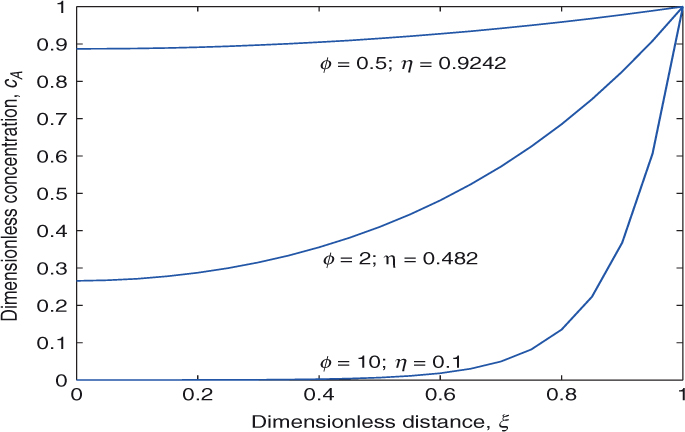
Figure 18.1 Concentration profiles for a first-order reaction in a catalyst in a slab shape. Dirichlet condition used at ξ = 1.
Slab: External Transport Effects
The solution for any general case where a Robin condition applies is slightly lengthy:
The reader may wish to verify the algebra and also show that the Dirichlet limit is approached as Bi → 1. Such limiting cases should always be checked in general.
The effectiveness factor expression for the above case can be derived as
Long Cylinder: Dirichlet Problem
The governing equation for a cylinder in dimensionless form is
Here s = 1 the geometry parameter and ξ is the dimensionless parameter, r/R. Note that if s is set as zero the slab equation is recovered. Similarly if s = 2 the model for a sphere is obtained.
The previous differential equation for a cylinder is now the modified Bessel equation. This can be seen by expanding the Laplacian and rewriting the equation as
The general solution is
cA = A1I0(ϕξ) + A2K0(ϕξ)
Students may wish to verify the general solution using MAPLE or the information given in advanced engineering mathematics textbooks such as Kreyzig (2010).
The constants of integration are readily found for a solid cylinder. The function K0 goes to infinity as r → 0 and hence A2 is set as zero so that the concentration remains finite at the center. The second constant is then fitted from the boundary condition at ξ = 1, which may be of the Dirichlet or Robin type. For the Dirichlet type (infinite Biot number) the solution is
The effectiveness factor is the ratio of the actual rate to maximum rate. The actual rate is the integral of the local rate multiplied by the local volume:
The maximum rate is
Maximum rate = πR2Lk1CA,s
L here is the length of the cylinder.
The ratio the two rates leads to the following expression in dimensionless version:
An alternative expression for the effectiveness factor is found from the flux crossing into the cylinder at the surface:
Students should verify that this will be the expression from flux considerations at the surface; both expressions will lead to the same final answer, which is
This is valid for large Biot numbers; that is, when the gas film transport is not rate limiting. The solution to the case of a finite Biot number is left as an exercise.
Sphere
Here Equation 18.8 applies with s = 2. A variable transformation f = ξcA reduces the equation to a form that can be integrated more easily (see exercise problem 1). The solution is
The effectiveness factor is given as
and the final result is
Example 18.1 shows an illustration of the drop in the concentration profile due to pore diffusion.
Example 18.1 Effectiveness Factor and Center Concentration in a Spherical Catalyst
A first-order reaction with a rate constant of 10 sec–1 is taking place in a porous spherical catalyst. The effective diffusion coefficient is estimated as 10–6 m2/s. Estimate the rate of reaction for a 1 mm and 5 mm diameter pellets. Also evaluate the center concentration for these cases to get a feel of the drop in the concentration in the pellet. Gas phase concentration is estimated as 30 mol/m3.
Solution
For the 1 mm case the Thiele modulus is calculated as 1.5811 and the corresponding effectiveness factor is 0.865. The rate is calculated as k1CAb η = 260 mol/m3s. The center concentration calculation requires taking the limit of Equation 18.10 and is equal to ϕ/sinh(ϕ). The value for a ϕ of 1.58 is 0.68, a 32% drop.
For the second case we have a Thiele modulus of 7.9057 and of 0.3315. The rate is only 99 mol/m3s now and the center concentration is 0.0058, a significant drop. The reactant is not able to reach the interior of the sphere.
Shape Normalization
A useful definition is the shape-normalized Thiele modulus. This definition can be used as an approximation for complex shapes. A full 3-D solution to the diffusion-reaction model may often not be needed.
We define a characteristic length parameter (equivalent half-length of a slab catalyst) as
Lc = Vp/Se
where VP is the volume of the particle and Se is the external surface for diffusion of the gas into the porous solid.
A Thiele modulus is then defined based on this length scale as
irrespective of the actual shape of the catalyst; the slab equation is used for all the geometries as an approximation with the above-defined Thiele modulus:
Note that ϕ* for a cylinder is ϕ/2 (the length parameter is now R/2). Similarly it is ϕ/3 for sphere. The length parameter is R/3. A plot of the effectiveness factor for all three geometries is shown in Figure 18.2.

Figure 18.2 Effectiveness factor for all three geometries plotted in terms of the shape-normalized Thiele modulus. + is a cylinder and * is a sphere from analytical solutions; the solid solid line is for a slab.
We find from this figure that the slab approximation is reasonable for all three geometries. The results for all three geometries get compacted with this modified (shape-normalized) Thiele modulus. The maximum error is on the order of 10% and is observed at an intermediate value of the Thiele modulus. The concept can be used for complex shapes; Example 18.2 shows one application.
Example 18.2 Annular Ring Catalyst
As an example, consider a catalyst shaped as an annular ring, with three dimensions: inside radius = Ri; outside radius = Ro; length = L.
The volume of the catalyst is , while the external surface area is the sum of the area at the top and the bottom of rings, the outer surface area, and the inner surface area:
Hence the equivalent length of the “slab” catalyst for diffusion is the volume of the catalyst divided by the external area:
Thiele modulus based on this length can be used and the slab model can be used as an approximation.
For a solid cylinder Ri = 0 and R = Ro; the length parameter is R/[2(1 + R/L)]. If L/R >> 1 this further reduces to R/2, the value of the characteristic length for the long cylinder case.
External Resistance
It is often useful to know if external resistance is important or whether it can be neglected and the simple Dirichlet condition used as the boundary condition.
At steady state the rate of external mass transfer is kmSe(CA,b – CAs), which is also equal to the rate of reaction in the interior of the catalyst, Vpk1CA,s η. The latter can be also represented as , which is the measured rate. Hence
If the rate is measured and the external mass transfer coefficient is measured independently or estimated from correlations we can find the concentration drop in the film from the previous equation. If the drop in the external film should be small relative to the bulk concentration, then the external mass transfer resistance can be neglected.
Apparent Rate Constant
The significance of η and the effect of Thiele modulus on the measured rate of reaction is discussed here.
Note that the local rate of reaction is k1CA(x) per unit catalyst volume. As the concentration is changing within the slab, the rate is different at different points in the slab. What one would observe is an average rate, which can be calculated using the definition of η. Hence
Using the expression for η (for the slab model with no external resistance)
an apparent rate constant can be defined as the observed rate divided by the bulk concentration. This is observed to be
which is not in general equal to the true rate constant k1. This indicates that the measured value should be appropriately corrected for diffusional effects. Example 18.3 illustrates this.
Two limiting cases are worth noting:
No pore resistance: This holds for low ϕ. The effectiveness factor = 1. The average rate, which is also the observed rate, is
The apparent rate constant and true rate constants are the same. The true rate constant can therefore be directly estimated from the measured data in this case. Also note that the particle size has no effect. One way to check this is to take two relatively small particle sizes. The measured rate will be the same if there are no pore resistances due to diffusion.
Strong diffusional resistance, which holds for high ϕ; Usually ϕ > 3 is taken as the criteria. Here we can show that η = 1/ϕ since the function tanh ϕ will now be one. Hence the measured rate would be
The apparent rate constant is now the bracketed term on the right-hand side. The rate is inversely proportional to the size of the catalyst. This is called the strong diffusional regime. A true rate constant cannot be directly obtained here but can be back-calculated if the effective diffusion coefficient is known or estimated. Example 18.3 illustrates the procedure.
Example 18.3 Correcting the Rate Constant for Diffusional Effects
Consider the problem examined in Example 18.1. Assume now that the rate constant is not known and the reaction rate is measured. For a 5 mm diameter particle, let the measured rate be 99 mol/s.m3. Find the true rate constant. To what extent is the internal diffusion resistance controlling? Assume a first-order reaction.
Solution
The gas phase concentration of A is fixed here as 30 mol/m3. Dividing the rate by the concentration, the apparent rate constant is known:
To find the true rate constant the extent of the internal diffusion coefficient in the pores must be measured or estimated. We use the value of 10–6 m2/s (same as in Example 18.1 for comparison purposes).
Based on the apparent rate constant, the Thiele modulus is calculated as 5.63. Hence η = 0.5331, which is only an approximate value. The reaction rate is calculated as kACAb η, 33 mol/m3s, which is far lower than the measured value.
If the rate constant is changed to 6, the rate can be recalculated. We calculate the rate to be 73 mol/s.m3. This is still lower than the measured rate and an increased value needs to be tested. A few trial and error calculations will zero in on the value of the rate constant to 10, which is the true value. The effectiveness factor is 0.3315 and the internal diffusion is strongly rate limiting.
Note: The reaction order is assumed to be first order. This may not be known a priori. In practice the rate will have to be measured at different concentrations to ascertain the reaction order.
18.2.2 Zero-Order Reaction
This is often important, especially in biological systems, as many metabolic reactions can often be approximated as a zero-order process. The zero-order kinetics is also observed in some hydrogenation reactions. Although the model equation is straightforward, special considerations are needed since the concentration value can actually become zero at some position in the diffusion path. This is unlike a first-order reaction where the concentration decays as an exponential function (which can of course become very small but never actually becomes zero). For zero-order reactions the concentration (a parabolic function as shown in the following) can actually become zero at some point within the porous catalyst, especially if diffusion is slow compared to the reaction rate. Hence we have to demarcate the position where the concentration actually becomes zero and analyze the problem separately in two regions. A simple example for a slab geometry is illustrated and other cases are left as exercises. An important problem application is in biomedical systems, that is, oxygen transport in tissues, which is also known as the Krogh cylinder problem. This is discussed in Chapter 23.
The slab analysis proceeds as follows with the basic diffusion-reaction equation:
where the production rate of A, RA, has been replaced by minus k0, the zero-order rate constant for the metabolic process. The boundary conditions are set as follows:
At x = L, CA = CAs, a prescribed or known surface concentration (Dirichlet case).
At x = 0, the center of the slab, we use the no flux condition dCA/dx = 0.
The dimensionless version of the previous equation can be easily derived as
Here is the square of the Thiele modulus for a zero-order reaction. This should be defined as
Note that the Thiele modulus depends on the surface concentration, unlike the case of a first-order reaction. This is true in general for any nonlinear kinetics.
The solution for the concentration profile (in dimensionless form) is very simple:
The center concentration is assumed to be above zero so that this equation can be applied.
The condition at which the center becomes zero or remains positive is then obtained from Equation 18.15 by setting ξ = 0 as
For this case, there is no reactant starved zone in the interior of the catalyst. The rate of consumption of A per unit volume is k0; this is independent of the concentration, as expected for a zero-order reaction. Hence the effectiveness factor is equal to one since the entire catalyst is exposed to the reactant as long as this condition is satisfied.
The solution for a larger Thiele modulus is studied next where a reactant starved region develops near the center of the catalyst.
Solution for Larger Thiele Modulus
For , the concentration becomes zero at a dimensionless location . The no flux condition is now imposed at ξ = λ since no mass of A crosses this point, rather than at ξ = 0. This leads to the following equation for the concentration profile:
The position λ is not known. Hence we impose an additional condition that the concentration cA is also zero at x = λ. This provides the following condition for the calculation of λ:
Note that only the region to 1 is effective for a reaction. Hence the effectiveness factor is simply the length of the region and can be calculated as
The rate of consumption of A per unit volume is now k0 η and turns out to be
This shows a square root dependency on the surface concentration. Thus a zero-order reaction appears as a half-order reaction due to the presence of diffusional effects.
This is a general effect and can be stated as follows:
A reaction of true order n appears as a reaction of (n + 1)/2 when strong pore diffusional resistances are present.
The concentration profiles for various ranges of the Thiele parameter are shown in Figure 18.3.

Figure 18.3 Concentration profiles for a zero-order reaction in a porous catalyst for three values of the Thiele parameter.
In Figure 18.3 three cases are shown. The first case is for ϕ0 = 1 and represents the no starvation case; the concentration remains finite everywhere. The second case is for . The concentration becomes zero at the center; this represents the onset of starvation. The effectiveness factor is one for both these cases. The third case is for ϕ0 = 3 and represents a case of strong diffusional gradients. The concentration becomes zero at ξ = 0.53. The region from 0 to 0.53 is not effective for the reaction. The effectiveness factor is equal to 0.47, the width of the zone where the reactant concentration is non-zero.
Similar to a zero-order reaction, reactions with power law order less than one can exhibit a depleted zone near the center. The analysis of this problem was undertaken by Mehta and Aris in 1971 following the work of another earlier researcher and resurrected in 2011 by York et al. (2011). The mathematical method to find the critical Thiele modulus is examined in exercise problem 10.
We now move to a nonlinear nth-order reaction and illustrate a mathematical solution method for such problems for large values of the Thiele modulus. The corresponding result for the effectiveness factor is known as the asymptotic solution.
18.2.3 nth-Order Reaction
In this section we show a variable substitution method for a nonlinear diffusion reaction problem and derive a solution for large values of the Thiele modulus. In order to illustrate the key points, we take an nth-order reaction and show the derivation directly in dimensional form for a slab geometry. The Dirichlet condition is also used at the surface.
Expression for the Surface Flux
Consider diffusion with an nth-order reaction in a porous catalyst, which can be modeled for a slab geometry as
The order of the differential equation can be reduced by one by using the transformation p = dCA/dx. (Hence the method of solution is called the p-substitution.) Noting that
we find that Equation 18.18 can be written as
This equation can be solved by separation of variables to get an expression for p, the concentration gradient:
or
The limits are set as follows. For flux the limits are set as 0 at the center and the unknown surface gradient ps. For concentration the unknown center concentration and the known surface concentration are used.
Note that the center concentration is unknown but an expression can be derived in integral form upon a second integration. However, these details are not important in the asymptotic region, which applies for large values of the Thiele modulus. Here the concentration drops to nearly zero at some point in the interior of the catalyst. Thus we can set CAc ≈ 0 and use this in the above expression. The flux at the surface is then given as
Taking the square root with the positive sign (since the concentration is increasing with increase in x), we obtain an expression for the surface gradient:
The quantity entering the catalyst is given as
Correspondingly the average rate of reaction is obtained as
Using Equation 18.24 for ps, the following expression is obtained for the average rate:
Note that this reduces to Equations 18.12 and 18.17 for first-order and zero-order reactions with n equal to 1 and 0, respectively.
Effectiveness Factor
The expression for the average rate can be put in terms of an effectiveness factor. This is given by the ratio of the actual rate to that based on surface concentration (only internal gradients considered):
Therefore the following expression holds for the effectiveness factor upon using Equation 18.27 in the asymptotic region:
Note that η = 1/ϕ for a first-order reaction in the asymptotic region. Now if we wish to write the previous result for an nth-order reaction in a similar format as: η = 1/Λ, the Thiele modulus Λ should be defined as
This is known as the kinetic generalized Thiele modulus. Now we have η = 1/Λ for any kinetics, but only for the asymptotic case.
The expression for η is then generalized as
This expression is strictly valid only in the asymptotic region where tanh(Λ) tends to one but is used for the entire range of Λ values as an approximate solution.
Further, shape normalization can be introduced in order to apply this to other shapes as well. The length parameter is now changed to Vp/Se and the Thiele modulus is further generalized as
The expression for η given by Equation 18.29 is then used for the nth-order reaction as an approximation for the entire range of Thiele values and for any shape of catalyst. This approximate method of calculation of the effectiveness factor is known as the Bischoff (1965) approximation.
18.3 Multiple Species
Here we examine two species reacting together. Diffusion equations for both species are needed and must be solved simultaneously. Multiple reactions can be handled in the same manner.
The following reaction scheme is used in the the analysis presented in this section:
A + νB → Products
The diffusion equations for species A and B both have to be solved together here. Both of these concentrations are lower in the pellet compared to the surface. We illustrate the method by taking a slab geometry and a bimolecular (1,1) order reaction. Note that a product concentration increase in the pellet can also be computed by a similar procedure.
The model equations to be solved are as follows for components A and B:
and
The concept of a limiting reactant is very useful here. The reactant whose value of its surface concentration times the diffusivity is lower than the other is usually the limiting reactant. Species A is limiting if
and vice versa. The second species is called the excess reactant. For further discussion A can be assumed to be limiting without loss of generality. Thus if B is limiting, the notations can be switched.
One of the important relations that is useful here and also in a general context is the invariant property of the equations. Thus by combining the equations for A and B where we have the common rate term we find the following relation holds between the concentrations of species A and B:
The integrated form suggests that
Hence CB (the excess reactant) can be eliminated in Equation 18.31 and a single differential equation can be solved for A only. The number of differential equations to be solved is thus reduced to one. In the asymptotic region an analytical value can also be obtained by the p-substitution method since we have only one differential equation to handle. An illustrative result is shown in Figure 18.4.
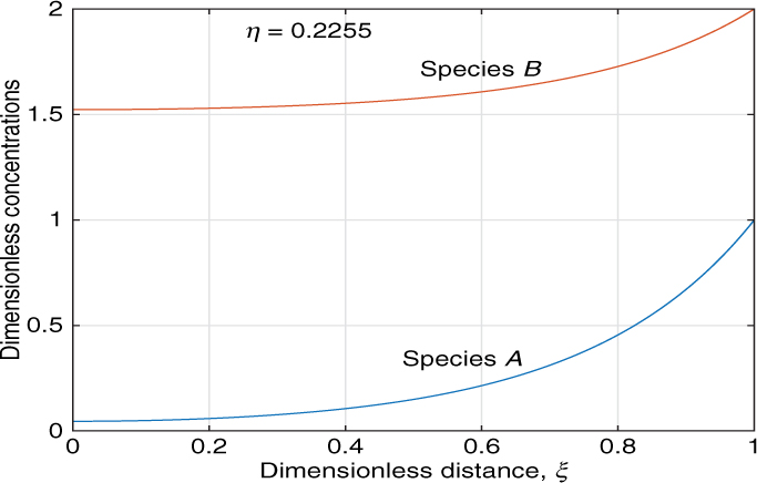
The results shown in this figure are for a slab geometry with ϕ = 3 and q = 2.0. Here species B is the excess reactant since q > 1. Note that the concentration of the excess reactant (B) drops only marginally in the catalyst while that of the limiting reactant drops much more significantly here. The effectiveness factor can be calculated as 0.2255 for this case. Analysis for multiple reactions follows a similar methodology.
18.4 Three-Phase Catalytic Reactions
A large class of industrially important examples include three phases: gas, liquid, and a solid catalyst. Transport of a species from the gas phase and transport of a second species from the liquid are often the rate determining steps. This section provides a brief introduction to mass transport effects in three-phase systems. A simple first-order reaction is considered and transport effects are accounted for by a resistance in series approach. For more details a complete textbook (Ramachandran and Chaudhari, 1983) and many other monographs are available. We first cite some industrial examples and some common reactor types.
18.4.1 Application Examples
Some examples of industrial-scale gas–liquid–solid catalyzed reactions are the following:
Hydrogenation reactions: Examples include hydrogenation of glucose to sorbitol, unsaturated oils, nitrocompound, aldehydes and esters, and so on.
Hydrodesulfurization of diesel to remove sulfur compounds.
Hydrocracking of petroleum fractions using supported metal catalysts to produce lower molecular compounds, such as the gasoline fraction from heavy oil.
Methanol synthesis from a CO and H2 gas mixture in the liquid phase with suspended solid catalyst.
Fisher-Tropsh synthesis from syngas to produce fuels where synthesis gas (CO, H2 mixture) is converted to heavy hydrocarbon fractions.
Oxidation reactions; these include oxidation of cumene, phenol, p-xylene, and so on, using oxides of Cr, Cu Co, and so on, as solid catalysts. Note that use of soluble homogeneous catalysts is more common for oxidation and such reactors belong to the category of two-phase reactors.
Reactor Types
The common industrial reactors can be classified into the following types:
Slurry type: Here the catalyst particles are suspended in a liquid with gas being simultaneously sparged into the liquid. The dispersion of the gas and the suspension of the solid catalyst can be done simply by bubbling the gas (bubble column reactor) or by mechanical agitation.
Fixed bed type: Here the catalyst is stationary and the gas and liquid flow over the catalyst bed similar to a packed bed absorption column. The flow may be cocurrent downward (e.g., trickle bed reactor shown in Figure 1.4) or concurrent upflow (packed bubble column reactor) or countercurrent flow over a packed catalyst bed.
Relative comparisons and the choice of reactors are discussed by Ramachandran and Chaudhari (1983), Mills et al. (1992), and other references; these should be consulted if you are designing these types of reactors. The focus here is mainly on mass transfer effects and how the effectiveness factor concept is useful to calculate the rate of reaction for a simple first-order reaction.
18.4.2 Mass Transfer Effects
For the simple case shown in Figure 18.5, a number of steps have to occur before species A can be converted on the active sites for production:

Figure 18.5 Mass transfer effects in three-phase catalytic reactors S-L means solid liquid; R = radius of the catalyst particle.
Transport of gas from bulk gas to the bulk liquid. This can be modeled using an overall mass transfer coefficient from gas to liquid:
is the saturation solubility of the gas in the liquid based on the bulk gas concentration of gas A. CAL is the concentration in the bulk liquid. The is the volumetric absorption of A in the system which equals the rate of reaction of A per unit reactor volume. This step has a resistance of 1/KLagl.Transport of dissolved gas from the bulk liquid to the catalyst surface. This can be modeled using a solid–liquid mass transfer coefficient:
Here kls is the intrinsic liquid–solid mass transfer coefficient and als is the external surface area of the catalyst per unit reactor volume. This step has a resistance of 1/klsals.
Internal diffusion with reaction. This can be modeled using k1 η as the rate coefficient:
A simple first-order kinetics is used here. w is the mass of the catalyst per unit reactor volume. This step has a resistance of 1/wk1 . The rate constant k1 here is defined on the mass of the catalyst.
Usually species A will react with a second liquid phase B, which gets transported to the catalyst as well. However if the second species is in excess, the reaction may be approximated as pseudo-first-order case shown here. The details of surface interactions such as adsorption on the active surface followed by reaction are also lumped into the rate constant. The effect of pore diffusion is captured by using the effectiveness parameter, which in turn depends on the Thiele modulus.
Each of the transport steps contribute to a corresponding resistance. For a linear process the resistances can be added. The overall rate can be then calculated as
where ηc in turn can be calculated based on the Thiele parameter for the catalyst.
18.5 Temperature Effects in a Porous Catalyst
In this section we show the transport effect where an exothermic reaction is taking place in the catalyst. Due to the release of heat due to the reaction, a temperature profile develops in the catalyst. This in turn affects the rate of reaction via the Arrhenius dependency of the rate constant on the temperature.
18.5.1 Equations for Heat and Mass Transport
The simultaneous transport of heat and mass in a porous catalyst is needed for analysis and can be represented by the following set of equations for a slab geometry:
where ke is the effective conductivity of the catalyst and ΔH is the heat of reaction. The local rate of disappearance f(CA, T) is now a function of both the pore concentration and the temperature at any point in the pellet.
The boundary conditions are specified as follows: no flux condition is imposed at the pore end (x = 0) for both heat and mass:
at x =0 dCA/dx = 0; and dT/dx = 0
At the pore mouth (x = L) the flux into the pellet must match the transport through the gas film. This leads to the following boundary conditions:
For mass transport:
For heat transport:
18.5.2 Dimensionless Representation
The equations can be put in terms of dimensionless variables by scaling the concentration and temperature by reference values. The bulk concentration and temperature can be used as reference values if the particle-scale model is being analyzed. For reactor-scale models, the inlet feed conditions can be used as a reference.
The dimensionless mass and heat transport equations are then as follows: the mass balance equation is
Here f* is a scaled rate of reaction, defined as
f* = f(CA, T)/[f(CAref , Tref)]
ϕ2 is a Thiele modulus based on reference conditions:
The dimensionless heat balance equation is
where β is the dimensionless parameter (thermicity group), defined as
Note that β takes a positive value for exothermic reactions and a negative value for endothermic reactions.
The dimensionless rate has to be appropriately defined, including the temperature effect on the rate constant. For example, using the Arrhenius equation, the dimensionless rate for a first-order reaction can be expressed as
where γ = E/RgTref . E is the activation energy for the reaction. Parameter is a dimensionless group sometimes referred to as the Arrhenius number. The governing equations and the boundary conditions shown in Section 18.5.1 to be solved are then calculated as follows. The species mass balance is:
and the heat balance is
18.5.3 Dimensionless Boundary Conditions
The normalized boundary conditions can be stated as follows.
At the center the no flux condition is used for both the concentration and the temperature:
At ξ = 0, dcA/dξ = 0; d /dξ = 0
The conditions at ξ = 1 can be related to the Biot numbers for heat and mass:
Here the subscript s is used for ξ = 1, that is, the surface values. The subscript g is used for the bulk values. For the particle problem (local particle-scale model) we can set cg and θg as one since the reference concentration and temperature are the bulk values.
The Biot numbers for mass and heat are defined as
Bim = kmL/De
and
Bih = hL/ke
This completes the problem formulation. The problem requires a numerical solution in general.
The results are often shown in terms of an effectiveness factor as a function of Thiele modulus, defined as
Even for this simple first-order reaction, the overall effectiveness factor is a function of five parameters shown previously. It is a numerical problem with a daunting solution and has been the subject of many research papers. However, certain features can be examined even without solving the full set of equations. Let us now examine if we can calculate the maximum temperature rise (exothermic case).
18.5.4 Estimate of the Temperature Gradients
The magnitude of the internal temperature gradient can be assessed by combining the two differential equations, Equations 18.39 and 18.40, without even actually solving for the full temperature profiles. These mass and heat transport equations can be combined as
Hence the integration of this equation twice leads to
This is an invariant of the system.
The maximum value of the temperature occurs for an exothermic reaction when the center concentration drops to zero. This occurs in the strong pore diffusion resistance for mass transfer. Hence an estimate of the internal gradients is
Here θc is the center temperature. Further the maximum value of cAs is one. Hence the dimensionless maximum temperature difference between the center and surface is β. Using dimensional values we find the following expression:
The maximum difference occurs when CAc is nearly zero; hence this analysis provides a quick method of calculating the maximum internal temperature that can develop in the catalyst.
The temperature rise across the gas film can be related to the measured rate of reaction if an estimate of the film heat transfer coefficient is made. This is simply a heat balance across the gas film, which is observed by rewriting this as
The left-hand side is heat transferred from the solid while the right-hand side is the heat generated due to reaction in the pellet. Note that Vp/Se is the characteristic length parameter, Lc.
The above relations enable a rapid determination of the relative importance of external and internal temperature gradients. It can be, for instance, used to determine whether the pellet is operating under near isothermal conditions or whether a temperature correction to the data is necessary.
Detailed numerical results for various combination of parameters can be generated, for example, using BVP4C with MATLAB. The solution can show multiple steady states for a certain range of parameters and the effectiveness factors can be larger than one. This happens only for an exothermic reaction where the interior of the catalyst is hotter than the bulk gas. The rate increase due to temperature rise can often compensate for the rate decrease due to concentration increase. This can cause effectiveness factors to be greater than one.
In the next two sections, we discuss two numerical tools to solve diffusion-reaction problems. The first tool is based on orthogonal collocation and is suitable for 1-D problems in the three standard geometries. The second tool is a finite difference method and is suitable for 2-D and 3-D problems.
18.6 Orthogonal Collocation Method
Collocation methods are powerful and accurate tools for the solution of diffusion-reaction problems. The goal of this section is to provide a brief introduction to the method together with a worked example. The detailed theory behind the collocation method is beyond the scope of this book. The interested reader should refer to Villadsen and Michelson (1978).
18.6.1 Basis of the Method
The method is based on expansion of the solution variable, denoted here as c, in terms of orthogonal polynomials in the distance variable, ξ. We select a number of collocation points, which are the roots of the Jacobi polynomial defined in an optimum manner. It may also be noted here that for problems with symmetry at ξ = 0, it is not required to select the point ξ = 0 as a collocation point. This is because the expansion uses polynomials with even powers in ξ and hence the symmetry boundary condition is automatically satisfied.
Collocation points are chosen differently for each of the three geometries so as to minimize the error in the calculation of the average rate of reaction or equivalently the effectiveness factor. Again these details are not addressed here as the main theme is to demonstrate the numerical implementation of the method and to provide useful code. The key result needed from the user point of view is that the Laplacian at each interior collocation point (or node) is approximated as an algebraic equation as shown in Figure 18.6.
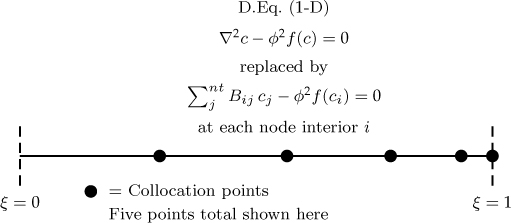
Figure 18.6 Representation of the collocation approximation to the diffusion-reaction problem. Note: cA is abbreviated as c; f is the dimensionless form of the rate of reaction term.
This equation, known as the discretization formula, is applied at all interior nodes, that is, i = 1 to nt – 1, generating a set of algebraic equations. The discretization is not applied at the boundary node at ξ = 1. Instead the set of equations is augmented by applying the boundary condition at the node designated as nt. This may be a simple Dirichlet for concentration (c = 1) or a Robin boundary. A Robin boundary needs an approximation of the first derivative, which is given by the A matrix:
Thus nt equations for nt variables are obtained. This set of nonlinear algebraic equations can be solved in an iterative manner by the Newton-Raphson method, which requires the linearization of the rate term f(c) at each level of iteration.
18.6.2 Two-Point Collocation
Often when the concentration profiles are not too steep, a single interior point collocation is sufficient. Together with the boundary, this is known as a two-point collocation and provides a quick method for calculation of the effectiveness factor. Example 18.4 demonstrates this for a spherical geometry with a simple first-order example for which an analytical solution is also available for comparison.
For a sphere the values of the A and B matrices for a two-point collocation are listed in the following. In addition, the quadrature weights w to approximate the integral of the concentration and the location of the points ξ are also given.
Example 18.4 Two-Point Approximation
Solve the diffusion-reaction problem for a first-order reaction in a spherical geometry with one-point collocation in the interior of the pellet and compare the results with the analytic solution.
Solution
We apply the collocation at one interior point:
B11c1 + B12c2 = ϕ2c1
If the Dirichlet condition is applied at the surface, c2 = 1. Hence we get the concentration at the interior point:
The effectiveness factor is then calculated using the quadrature weights as
η = (s + 1)[w1c1 + w2c2]
For a specific value of ϕ = 2 we get the following results using the matrix coefficient values reported in Table 18.1:
c1 = 0.7241 and η = 0.8067
Table 18.1 Collocation Matrices for Two-Point Collocation for Sphere
A =[ -2.2913 2.2913 -3.5000 3.5000] |
These can be compared with the analytical values, which are 0.7231 and 0.8069. We see a pretty close match.
If ϕ = 5 we get η = 0.5070, which is also close to the analytical value of 0.4801. The concentration at the interior point is now 0.2958 while the analytical value is 0.2713.
For a second order reaction with the Dirichlet condition at the surface, the one point representation would be as follows:
This can be solved as a quadratic. The effectiveness factor can then be calculated using the quadrature weights.
Note: Often reactors are operated in the intermediate range of the Thiele modulus and one (interior) point is sufficient for many practical purposes.
18.7 Finite Difference Methods
Finite difference methods are simple to apply for regular geometries, which are defined as geometries where the sides are parallel to the coordinate axis, that is, there are no curved boundaries. These include square- or rectangular-shaped domains or L-shaped or similar domains in 3-D. Domains with curved boundaries (e.g., an ellipse) need special treatment for the second derivative near the boundaries and are not considered here. There are many sources for the interested reader to pursue this topic further.
Consider the solution of the following problem:
Here x and y are treated as dimensionless variables. cA is a dimensionless concentration and ϕ is the Thiele modulus.
The domain is divided into meshes along the x- and y-directions with a chosen scale Δx and Δy in each direction. We now abbreviate cA by c.
18.7.1 Central Difference Equations
The second derivatives are approximated by central difference approximations presented in the following.
In the x-direction the approximation at node i is
Similarly in the y-direction we use
Hence the finite difference discretization applied at node (i, j) leads to
For direct iteration purposes, the equation is rearranged with c(i, j) as the term on the left-hand side and with all the other terms moved to the right-hand side:
Here the old values (values at previous iteration) are used on the right-hand side and these are known. This permits the calculation of c at node (i, j) (the new value). By sweeping over all the nodes one round of iteration is completed and all the old values are replaced by the new values calculated using the left-hand side of the preceding equation. This sets up an iteration scheme that converges to the solution after a few rounds of updating the concentration values. Illustrative results are shown in Figure 18.7.

Figure 18.7 Concentration profiles for a first-order reaction in a square catalyst shown as contour plots; ϕ = 3. Dirichlet condition: c = 1 is applied along the boundaries.
The contour plots of the results in Figure 18.7 are for ϕ = 3. The center concentration is found to be equal to 0.5614. The effectiveness factor can be computed either from the average concentration or by calculation of the flux values at the boundary. Both approaches will give (nearly) the same result. The value is 0.7899. A shape-normalized approach gives a value of 0.8469.
18.7.2 Zero-Order Reaction
The simulation for a zero-order reaction is done in a similar manner. Here f(c) = 1. Also the Thiele parameter is renamed ϕ0.
The iteration scheme now is
The results are shown in Figure 18.8 for ϕ0 = 3. If this parameter is increased you will find a region of negative concentration in the center of the system. This indicates the onset of starvation. It can be shown that a Thiele modulus of 3.685 leads to starvation.

Figure 18.8 Concentration profiles for a zero-order reaction in a square catalyst shown as contour plots; ϕ = 3. Dirichlet condition: cA = 1 is applied along the boundaries.
18.7.3 Nonlinear Kinetics
Nonlinear kinetics can be determined by local linearization. Consider the rate term ϕ2f(c). This is linearized based on the current iteration values as
The two coefficients κ0 and κ1 are obtained by Taylor series approximation at the current value of the nodal concentration, denoted as c*A here:
and
In the iteration scheme κ0 is treated as a zero-order reaction term and κ1 as a first-order term. These terms change values during each iteration as they depend on the current value of the nodal concentration. Hence the iteration scheme is a combination of a first-order and a zero-order reaction.
For, example for a second-order reaction and we have and where * denotes the old values, that is, the values at the previous iteration. The κ0 and κ1 are adjusted at each iteration until the iteration values at all the nodes converge.
18.7.4 Neumann and Robin Conditions
We now show how other types of boundary conditions can be used. Along the boundaries perpendicular to the x-direction we approximate the normal gradient as
Here s is the surface node, s – 1 is the next node adjacent to it, and s – 2 the third node from the surface.
If a no flux condition is applied at the Neumann boundary node, the normal flux is set to zero and concentration values at the surface node are given as
Thus the surface values for these nodes are updated using this equation at each iteration along with the interior values.
Along a Robin boundary the boundary condition is
Using Equation 18.52 as the approximation for the normal derivative and rearranging, the following expression is obtained for the surface concentration:
where Δs is the mesh spacing at these nodes. Thus along a Robin boundary the iteration is adjusted to maintain this value for cs.
18.8 Linking with Reactor Models
This section provides a simple example where the local model for the porous catalyst is linked to a reactor model to demonstrate how models at two scales are linked. More complex cases (not shown here) follow simply by extension of the method.
A model for a plug flow case is considered here for an isothermal system with no appreciable change in gas velocity. The species mass balance equation based on a mesoscopic control volume is
In – out + generation = zero
The generation is calculated as the rate of reaction based on the local gas concentration (and temperature for non-isothermal reactions) times the local effectiveness factor. The effectiveness factor accounts for the effect of concentration drop within the catalyst and in the gas film as well. The rate of reaction is based on the volume of the catalyst. Since the mass balance is based on the total control volume (gas+solid) the rate should be multiplied by the catalyst volume per unit bed volume (1 – ∊B) with ∊B being the bed porosity, that is, the volume of the gas per unit volume of the bed. Putting all this together the generation term is
Generation = (1 – ∊B)RA(gas)η
RA(gas) is the rate of reaction based on the local gas concentration at a given point in the reactor. The effectiveness factor thereby couples the reactor-level and particle-level models. The mass balance for the concentration CA in the gas phase is therefore
This can be integrated by a finite difference marching scheme in z or by any solver such as ODE45. The point to note is that is a function of local concentration CA (unless the reaction is first order at isothermal conditions). Hence at each point of the integration scheme, the value of has to be calculated and incorporated in the marching scheme. For a non-isothermal reaction both mass and heat balance for the gas phase has to be solved together with the effectiveness factor computed from the particle scale model shown in Section 18.5 locally at each axial location. This is a challenging computational problem.
A simple illustration for a power-law kinetics under isothermal conditions is provided in the following. The kinetics is represented as . The gas phase balance is
This is written is dimensionless form as
where ζ is z/L, the dimensionless distance. The parameter Da is the Damkohler number, defined as
The calculation of η can be simplified by using the generalized Thiele modulus. For a nth-order reaction the Thiele modulus is proportional to as can be garnered from Equation 18.28. Hence the local Thiele modulus can be written in terms of the inlet Thiele modulus Λi as
The effectiveness factor can be calculated as tanh(Λ)/Λ at each location. Using these in Equation 18.54, the concentration change in the gas phase is given by the following differential equation:
This is now in a form ready for the ODE45 solver. The reactor exit conversion is now dependent on two dimensionless parameters: Damkohler number and the inlet Thiele modulus.
18.8.1 First-Order Reaction
The computation is easy for first order since the Thiele modulus is not a function of the local gas concentration, CA. Hence calculated based on the inlet Thiele modulus is valid throughout the reactor. Hence Equation 18.53 can be directly integrated analytically:
cA,e = exp[–(1 – ∊B)k1 ηL/uG]
The equation resembles a plug flow reactor and is often represented as
Here kapp is an apparent rate constant:
kapp = (1 – ∊B)k1 η
Equation 18.56 can be used to fit the reactor data, but the fitted value of apparent rate constant is not a true rate constant and will in this case vary with particle size if internal gradients are rate limiting. Hence corrections for the internal diffusional effects have to be applied to get the value of the true rate constant.
18.8.2 Second-Order Reaction
An illustrative result for the exit concentration for a second-order reaction is shown in Table 18.2 using numerical integration of Equation 18.55 with ODE45.
Table 18.2 Exit Concentration in a Packed Bed Reactor for Power-Law Kinetics
Λi |
n = 1 |
n = 2 |
0.1 |
0.0503 |
0.2503 |
1.0 |
0.1017 |
0.2786 |
10.0 |
0.7408 |
0.7561 |
The results are for Da = 3 for various values of the inlet Thiele modulus. The effectiveness factor varies along the reactor for a second-order reaction, is lower near the inlet, and increases toward the exit of the reactor for a second-order reaction. This is accounted for in the numerical scheme. For low values of the inlet Thiele modulus, the effectiveness factor is one throughout and an exit concentration is 1/(1 + Da) or 0.25 is observed. The corresponding conversion is 75% At high values of the Thiele modulus, internal diffusion limits the rate and the conversion is only 25% at the same gas residence time.
18.8.3 Zero-Order Reaction
The case of the zero-order reaction is rather interesting. In the absence of internal gradients, a value of Da = 1 is sufficient for complete conversion. This is not so in the presence of internal diffusion. At some point in the reactor a critical value of the Thiele modulus of (for slab) is reached. The point where it is reached depends on the inlet value of the Thiele modulus. If the inlet Thiele is 1 then the critical value is reached at a point where the concentration is 0.5. Diffusional effects start to play a role beyond this point. The exit concentration of 0.22 is reached for this and complete conversion is not achieved. It may also be noted that beyond the critical concentration, the reaction would exhibit an apparent order of one half rather than the intrinsic order of zero.
Summary
Mass transfer with reaction in a porous catalyst is an important problem in reaction engineering. The model (when applied to catalysts of simple shapes) leads to second-order ordinary differential equations of the boundary value type.
The concentration profile within the porous catalyst depends on a dimensionless parameter, the Thiele modulus. Small Thiele modulus values lead to an almost uniform profile in the catalyst, leading to a complete utilization of all of the catalyst. For large Thiele modulus values, the concentration profile is confined to a thin region near the surface and only this part of the catalyst is being used for reaction. An effectiveness factor can be defined as the rate of reaction divided by the rate based on the bulk concentration. This is a measure of the effect of the internal gradients on the rate of reaction.
Mass transfer accompanied by a zero-order reaction has some special features. Here the rate is not affected by diffusion and remains constant up to a critical value of the Thiele parameter. Beyond this the rate is affected by diffusional gradients. The problem has important applications in oxygen transport in tissues, some hydrogenation reactions, and growth of microbial cells, which often follows a zero-order metabolism.
Catalysts of different shapes (rings, trilobes, quadrilobes, wagon wheels, and so on) are commonly used in industrial reactors. The motivation is to reduce the pressure drop using larger sizes but at the same time keep the interior accessible to the reactant. For these complex shapes, a slab type ratio of model is used as an approximation with an effective length parameter defined as the volume to the external surface area of the catalyst.
For nonlinear reactions a generalized Thiele modulus can be defined and used to find the effectiveness factor. This provides an approximate way of executing the calculation without needing to solve nonlinear differential equations. The procedure is especially useful to couple the particle-scale model to a reactor-level model.
Multiple reactions are handled by solving the diffusion-reaction model for each species. Simplifications based on the invariance property of the system of equations can be used. The number of species balances to be solved is equal to the number of independent reactions. The species balances for the other species simply follows from the stoichiometry of the set of reactions.
Systems with three phases (gas, liquid, and solid) are common in industrial practice. Additional transport effects (gas–liquid and liquid–solid mass transfer) are included in the analysis in addition to intraparticle diffusion and reaction. For a first-order reaction, the resistances of each transport step can be added and the rate can be calculated by dividing the driving force by the total resistance.
Reactions in porous catalysts can be accompanied by temperature changes and lead to a coupled problem in heat and mass transfer. Temperature rise for exothermic reactions causes an exponential rise in the rate of reactions, leading to many complexities such as multiple steady states, large sensitivity to small changes in parameters, and so on. Even for a simple first-order reaction, five dimensionless parameters are needed in the model formulation.
The orthogonal collocation method is a very fast and simple method for diffusion-reaction problems posed in slab, cylinder, or sphere geometries. The collocation points are chosen in such a manner that the result for the effectiveness factor is as accurate as possible for the given approximation. A symmetry condition is implicit in this formulation and need not be applied as a boundary condition. This is a numerical tool well worth learning. Often one (interior) point collocation is sufficient to give accurate results for moderate values of the Thiele modulus.
The finite difference method is another useful tool especially for 2-D and 3-D geometries. Due to the elliptic nature of the differential equation, a method based on successive relaxation is useful and provides a simple computational tool for these problems. These can be implemented easily on the MATLAB platform.
Particle-scale models provide a submodel for linking with reactor-level macro- or meso-level models. Mixing at the reactor scale needs to be assumed. Thus the gas phase can be in backmixed or plug flow for the two ideal cases. Reactor performance is usually bracketed between these values. The variation of the effectiveness factor along the reactor position needs to incorporated into the reactor model unless the reaction is first order and isothermal. If the reactor is assumed to be well mixed, the effectiveness factor should be calculated using the Thiele modulus based on the the exit concentration in the reactor.
Review Questions
18.1 What are the units for first-order, zero-order, and second-order rate constants if the rate is based on volume of catalyst, mass of catalyst, and surface area per unit volume of the catalyst?
18.2 How is the Thiele modulus defined and what is its significance?
18.3 If the concentration profile is known, state two ways of calculating the average rate of reaction for the catalyst.
18.4 Define the Thiele modulus for zero- and second-order reactions and verify dimensional consistency.
18.5 What is the Biot number and what role does it play in affecting the reaction rate in a porous catalyst?
18.6 Under what conditions does the rate of reaction become dependent on the catalyst size? Does it increase or decrease with size?
18.7 If the rate of reaction decreases linearly with catalyst size, what is the controlling resistance?
18.8 If the rate of reaction does not change with catalyst size, what is the controlling resistance?
18.9 What is the definition of the shape-normalized Thiele modulus? Why is it useful?
18.10 Can a zero-order reaction exhibit a dependency on the bulk gas concentration? If so, when?
18.11 Define the generalized Thiele modulus for an nth-order reaction.
18.12 A second-order reaction is taking place under strong pore diffusional resistance, that is, ϕ > 3. If the pressure is doubled by what factor would the rate change?
18.13 What dimensionless parameter is indicative of the maximum temperature difference between the center and the surface of a catalyst?
18.14 Can the effectiveness factor be larger than one? When?
18.15 A second-order reaction is taking place in a packed bed reactor. How would the effectiveness factor change along the axial length in the reactor?
18.16 A half-order reaction is taking place in a packed bed reactor. How would the effectiveness factor change along the axial length in the reactor?
Problems
18.1 Comparison of the three 1-D geometries. Consider the diffusion reaction problem represented in the three geometries. Verify the analytical solutions shown in the text for the three geometries with the Dirichlet condition of cA = 1 at ξ = 1 and the symmetry condition (Neumann) at ξ = 0. Note that the solution for a sphere needs a small coordinate transformation. (cA = f(ξ)/ξ, which reduces the governing equation to a simpler one in f.) Find the average concentration in the system for the three cases, which represents the effectiveness factor. Make a plot of the effectiveness factor versus ϕ* for all three cases where ϕ* is defined as a shape-normalized Thiele modulus defined as
Show that the results for the three geometries are quite close when is plotted as a function of ϕ*, which is referred to as the generalized Thiele modulus.
18.2 Robin boundary condition. Consider the same problem as above but now use a Robin condition at the surface. Derive an expression for the effectiveness factor as a function of Bi in addition to the ϕ parameter. Do the analysis for all three geometries.
18.3 Choosing an operating catalyst size. The rate of reaction was measured in a powdered catalyst of fine size and was found to be 200 mol/m3s. Assume the reaction to be first order and there are no internal gradients. The gas is at 1 atm and 400 K with a mole fraction of 0.1 for the reactant. Now we wish to change to a spherical pellet catalyst and we have an estimate of the effective diffusivity of the catalyst. De = 2 × 10⁻⁶ m2/s. From pressure drop considerations we wish to operate at a Thiele modulus of 0.4 or so. What should be the radius of the catalyst? How much will the catalyst effectiveness factor drop?
18.4 First-order catalytic reaction: effect of particle size. A first-order catalytic reaction was carried out with two different-sized spherical pellets and the following data was reported. For run 1: particle radius = 10 mm; observed rate = 3 × 10⁻⁵ mol reacted per cm3 catalyst per sec. For run 2: particle size = 1 mm; observed rate = 15 × 10–5 mol reacted per cm3 catalyst per sec. Estimate the Thiele modulus and the effectiveness factor for each of the above runs. Estimate the rate constant and the effective diffusion coefficient for this system. Use a bulk gas phase concentration of A as 100 mol/m3. Neglect gas side resistance.
Hint: Note that from the definitions the following relations can be deduced:
and
With these relations and the equation relating to ϕ you will be able to derive an equation for ϕ1 (or ϕ2); solve this and get the required results.
18.5 First-order catalytic reaction: strong pore resistance case. A first-order catalytic reaction was carried out with two different-sized spherical pellets and the following data was reported. For run 1: particle radius = 10 mm; observed rate = 3 × 10⁻⁵ mol reacted per cm3 catalyst per sec. For run 2: particle size = 5 mm; observed rate = 6 × 10⁻⁵ mol reacted per cm3 catalyst per sec. Explain why it is not possible to estimate both the rate constant and pore diffusivity from this data. What can be estimated? Assume the bulk concentration is known.
18.6 Shape normalization. A first-order reaction has a rate constant of 5 sec–1 and is taking place in a catalyst with an effective diffusion coefficient of 10–6 m2/s. Use shape normalization to estimate the approximate value of the effectiveness factor for the following cases: (1) Long cylinder with a radius of 4 mm; (2) a short cylinder with a radius of 4 mm and a length of 4 mm; (3) a long annular cylinder with an outer radius of 4 mm and an inner radius of 2 mm; (4) a short annular cylinder with an outer radius of 4 mm, an inner radius of 2 mm, and a length of 4 mm. For case (1), compare the value with the exact answer.
18.7 Weisz modulus. For diagnostic purposes a dimensionless quantity called the Weisz modulus is useful. This is a combination of the Thiele modulus and the effectiveness factor and is defined as
ΦW = ϕ2η
Show that the Weisz modulus is related to the measured rate of reaction as
Hence conclude that it can be directly calculated from the measured rate. A measured value or estimated value of the internal diffusion in the pore is needed for this. Show that ifΦW < 0.4 or so the internal gradients are negligible and the measured rate is representative of the true kinetic rate constant. Replot the η versus ϕ plot as a η versus ΦW plot. What is the usefulness of this new plot?
18.8 Zero-order reaction in a sphere. Many hydrogenation reactions over Pd-supported porous catalyst show a zero-order kinetics. Consider such a reaction in a spherical catalyst. Show that the concentration at the center of the catalyst drops to zero if the Thiele parameter, defined as , is equal to . Here CAs is the concentration of the reactant (hydrogen) at the surface of the catalyst. Based on this conclude that the pore diffusional resistances are unimportant and the effectiveness factor is equal to one if the surface concentration is maintained above k0R2/6De.
18.9 Second-order reaction: sulfur removal from diesel. Sulfur compounds present petroleum fractions such as diesel that can be removed by contact with a porous catalyst containing active metals such as Mo in the presence of hydrogen. If the catalyst size is a sphere of radius 3 mm and the concentration of sulfur in the liquid surrounding the catalyst is 2 mol/m3 find the rate of reaction. Assume the reaction is second order in sulfur concentration with a volumetric rate constant of 0.5 m3/mol.s. The effective diffusion coefficient of sulfur compounds in the liquid-filled pores is estimated as 6 × 10⁻¹⁰ m2/s. Use a slab geometry as an approximation and find the characteristic length parameter L. Define and calculate the generalized Thiele modulus for this second-order reaction. Calculate the effectiveness factor based on the generalized Thiele modulus.
18.10 Fractional order: dead zones. Similar to the zero-order reaction, the fractional order reactions exhibit the existence of dead zones beyond a critical value of the Thiele modulus. The problem examines the derivation of this value.
Start with the dimensionless version of Equation 18.18 and use the p-substitution to eliminate ξ. Use the condition that if cA = 0 then p = 0 (i.e., a dead zone exists near the center) and derive an expression to get the following expression for the concentration gradient:
At the critical Thiele modulus ϕc, cA is just equal to zero at ξ = 0. Use this as the boundary condition, integrate the above equation by separation of variables and then show that the value of this modulus is
18.11 Porous catalyst with series reactions. Consider a porous catalyst with a series reaction represented as
A → B → C
Write governing equations for A and B. Express these in dimensionless form. Solve the equations for a case where the dimensionless concentration at the catalyst surface is one and zero for A and B respectively. Note: Both concentrations are normalized with the concentration of A at the surface. Calculate the dimensionless gradient for these two species at the surface. From these expressions calculate the selectivity parameter, defined as
S = –(dcB/dξ)/(dcAdξ) at ξ = 1
State the significance of this parameter. Plot S as a function of ϕ and show how the high selectivity changes with the Thiele modulus.
18.12 Bimolecular reaction: asymptotic solution. Derive an expression for the surface flux modulus for a bimolecular second-order reaction using the p-substitution approach. Show that the generalized Thiele modulus should be defined as follows:
Here ϕ* is the shape-normalized Thiele modulus, assuming the reaction to be pseudo-first order in species B, and q is the effective concentration ratio of B to A in the bulk gas.
18.13 Bimolecular reaction in a porous catalyst. Selective catalytic reduction of NOx with NH3 is studied in a porous catalyst of 4 mm diameter. The internal diffusivity was estimated independently as DA = 0.03 × 10⁻⁴ m2/s and DA = 0.05 × 10⁻⁴ m2/s. The reaction is second order with a rate constant of 2 m3/mol sec. The temperature was 600 K and the total pressure was 1 atm; the partial pressures of NO and NH3 were 500 kPa and 1000 kPa, respectively. Which reactant is limiting? Simulate the profiles in the interior of the catalyst. Find the effectiveness factor. To what extent is the diffusion limiting?
18.14 Hydrogenation of butynediol. Hydrogenation of butynediol was carried out in a slurry reactor with a Pd-based catalyst of size 0.01 cm with a catalyst loading of 0.2 kg/m3. The density of the catalyst is 1500 kg/m3. The reaction is bimolecular (first order with respect to both A and B) with a rate constant of 0.048 m6/kg kmol s based on the mass of the catalyst. The mass transfer parameters are as follows: kLagl = 0.3 s–1 and kls = 0.005 cm/sec for hydrogen and 0.009 m/s for butynediol. The diffusion coefficient is 0–9 m2/s for hydrogen. The Henry constant for hydrogen is 0.01 mol/m3 atm. The initial concentration of butynediol is 2.5 M. Find the time needed for 95% conversion of butynediol.
18.15 Internal and external temperature gradients. Catalytic cracking of gas oil is done at 903 K and 1 atm with a silica-alumina catalyst of 1.62 mm diameter. The effective diffusivity of the catalyst is 8 × 10⁻⁸ m2/s and the effective thermal conductivity of the catalyst is 0.36 W/m.K. The heat of the reaction is –167 kJ/mol and the activation energy is 176 kJ/mol. The mass transfer coefficient is 1 m/s and the heat transfer coefficient is 400 W/m2K. The measured rate is 0.4 mol/m3s. Estimate the internal and external temperature differences.
18.16 Second-order reaction in a packed bed. A second-order reaction is taking place in a packed column with 3 mm radius particles. The internal diffusivity is 10–2 cm2/s. The porosity of the bed is 0.4 and the rate constant is 0.75 m3/mol.s. The concentration of A in the feed is 12 mol/m3 and the volumetric flow rate is 0.5 m3/s. Find the reactor volume needed to get 90% conversion. What are the values of the effectiveness factor at the inlet and the exit of the reactor?
18.17 Two-point collocation for three geometries. The matrices needed for a slab and cylinder are shown in the following. The values for a sphere were shown earlier.
For slab geometry the values are as follows:
A = [ –1.1180 1.1180
–2.5000 2.5000]
B = [ –2.5000 2.5000
–2.5000 2.5000]
x = 0.4472 1.0000
w = 0.8333 0.1667
The values for the cylindrical geometry are as follows:
A = [ –1.7321 1.7321
–3.0000 3.0000]
B = [ –6 6
–6 6]
w = 0.3750 0.1250
x = 0.5774 1.0000
Use these to find the effectiveness factor for a second-order reaction with ϕ = 2 for all three geometries. Compare the results with the Bischoff approximation.
18.18 Collocation method for a reaction with substrate inhibition. A reaction with substrate inhibition can exhibit multiple steady states. As an example consider a diffusion-reaction model in a slab geometry with the following form: . Evaluate the effect of the Thiele modulus, keeping = 110 and = 1000. Compare simulation with two point and five point collocation method. Plot versus ϕ. Show that multiple steady states are likely for a Thiele modulus in the range of 23 to 26.8.
18.19 Collocation method with larger number of nodes. In Example 18.4 we showed the collocation method using only one interior point. This was found to be accurate for moderate values of the Thiele modulus, showing the power of the method. Here we wish to examine the solution for a larger number of points. The collocation matrices for nt = 5 for a slab geometry are presented in Table 18.3. Set up and solve the equations for various values of ϕ for a first-order reaction. Calculate as a function of ϕ with an analytical solution. Repeat for a second-order reaction. Compare the effectiveness factor to that calculated using the shape-normalized Thiele modulus. Verify that the five-point collocation is accurate for most practical applications, unless the Thiele modulus is extremely large. In latter case the asymptotic solution is good enough.
Table 18.3 Collocation Matrices for Five-Point Total Collocation for Slab Geometry.
A = -5.0717 8.6586 -6.3671 4.6458 -1.8656
-1.4346 -2.6538 6.3920 -3.7114 1.4077
0.5230 -3.1687 -1.9121 6.6239 -2.0661
-0.3861 1.8615 -6.7019 -1.6060 6.8325
0.7615 -3.4682 10.2684 -33.5618 26.0000
B = -34.4654 44.1493 -14.2677 7.0025 -2.4186
13.9798 -52.3162 48.8370 -15.1776 4.6771
-3.1083 33.6001 -94.5282 80.8944 -16.8579
1.8377 -12.5790 97.4469 -286.6901 199.9845
38.5462 -170.3650 457.9635 -794.1446 468.0000
w = 0.0251 0.0792 0.1152 0.0956 0.0182
x = 0.2958 0.5652 0.7845 0.9340 1.0000