Chapter 4. Examples of Mesoscopic Models

Search in book...
Toggle Font Controls
Create new playlist

Name your new playlist

Playlist description (optional)
Sign In

Email address

Password

Forgot Password?

or

Continue with Facebook

Continue with Google
Sign Up

Full Name

Email address

Confirm Email Address

Password

or

Continue with Facebook

Continue with Google

Chapter 4. Examples of Mesoscopic Models

Learning Objectives

After completing this chapter, you will be able to:

Apply the conservation law to a control volume that is differential only in the main flow direction.
Formulate mesoscopic models used in the analysis of mass transfer processes in tubular or channel flows.
Identify additional closures or assumptions to be made to complete the model.
Formulate and solve the simplest problem in mesoscale analysis— namely, solid dissolution from a wall.
Analyze tubular flow reactors and understand the model simplification using the concept of plug flow.
Understand the concept of dispersion and show how the plug flow model can be corrected using this parameter.
Set up models for systems with two flowing phases with interfacial mass transfer from one phase to another.
Show the application of the meso-model with two flowing phases to the simulation of a countercurrent gas absorption column.

Chapter 3 discussed macroscopic models. These models are useful when the system is nearly well mixed and therefore at a nearly uniform concentration. However, in many systems, the concentration varies predominantly and strongly in one direction, the flow direction. In such cases it is more useful to set up mesoscopic models. This control volume is a differential only in the main flow direction but spans the entire cross-sectional area in the direction normal to the flow. The concentration variable is then a flow-weighted cross-sectional area concentration or the so-called cup mixing concentration, rather than the point-to-point values of concentration. A differential equation can, in turn, be set up and solved for the variation of the cup mixing concentration as a function of flow direction. An illustrative problem is solid dissolution from a wall. In this first example in this chapter, we will demonstrate the model formulation for this problem. Knowledge of the mass transfer coefficient from the wall is needed as a parameter to close the model.

We next look at modeling of a continuous-flow reactor carried out in a pipe or a square channel. By the averaging process, we show that in addition to cup mixing concentration, the cross-sectional average concentration is needed in the model. Hence some closure relations are needed to relate the two average concentrations and thereby complete the model. The simplest closure based on a plug flow assumption is discussed first and some solutions to reactor performance based on this model are shown. We then introduce the concept of dispersion, which relates the two averages, and thereby closes the model. The results for reactor performance based on this dispersion model are then presented for a first-order reaction.

Additional examples of mesoscopic models in mass exchanger analysis are then presented. The first example is a single-stream mass exchanger. Here we have a membrane from which a solute is removed to an external fluid that stays at a constant concentration. The next example is a two-stream mass exchanger in which two flowing streams, say a gas and a liquid, exchange mass from one phase to another. The study of this problem assumes both phases involve plug flow and the problem has important applications in unit operations—for example, in simulation of gas absorption columns.

In summary, this chapter introduces a range of problems in mesoscopic mass transfer analysis mainly by examining specific examples. Through a careful study of these examples, you will be exposed to all the main tools used in mass transfer modeling of these systems. Further aspects of mesoscale modeling and the phenomena of dispersion are taken up in Chapter 14.

4.1 Solid Dissolution from a Wall

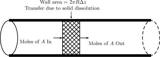
The problem we study in this chapter is mass transfer from a wall to a flowing fluid. A prototype example is a pipe coated with a soluble material and a liquid flowing in the pipe. The concentration of the dissolved solute at the exit of the pipe is to be calculated. Problems of this type and its variations have many applications and were introduced in Section 1.10.1; we continue the discussion here. This convection–diffusion problem can be analyzed based on a differential model (Section 10.1). Such models give pointwise concentration distributions—that is, C_A as a function of r and z. Often detailed information on concentration field may not be needed, and for such cases, we can simply use a mesoscopic control volume, as shown in Figure 4.1.

Diagram shows an example of a mesoscopic modeling.

Figure 4.1 Schematic of a solute coated pipe: an example of mesoscopic modeling.

4.1.1 Model Details

The model formulation involves the use of the conservation law, followed by a closure for the rate of mass transfer from the wall using the mass transfer coefficient. The conservation law applied to this system can be written assuming no generation and reaction as

in – out + transferred from the walls by solid dissolution = 0

This relationship is represented in symbols as

\begin{matrix} {\dot{M}}_{A, i} - {\dot{M}}_{A, e} + {\dot{M}}_{A, w} = 0 & (4.1) \end{matrix}

$\begin{matrix} {\dot{M}}_{A, i} - {\dot{M}}_{A, e} + {\dot{M}}_{A, w} = 0 & (4.1) \end{matrix}$

In the mesoscopic model, the in ${\dot{M}}_{A, i}$ ${\dot{M}}_{A, i}$ and out ${\dot{M}}_{A, e}$ ${\dot{M}}_{A, e}$ terms will be based on some radial averages of the local concentration. The formal definition of the concentration to use is presented in the following paragraphs.

We assume there is a velocity profile at any cross-section and let v_z be the local velocity at any cross-section. For example, in pipe flow, v_z would be a function of r, the local radial position. Local flow rate is therefore v_zΔA and local moles transferred across this area is C_Av_zΔA, where C_A is the local concentration. The rates at which the moles are crossing any given cross-section is therefore the integral of C_Av_zΔA over the cross-section:

\begin{matrix} Molar rate of transport of A across a cross-section = \int_{A} C_{A} v_{z} d A & (4.2) \end{matrix}

$\begin{matrix} Molar rate of transport of A across a cross-section = \int_{A} C_{A} v_{z} d A & (4.2) \end{matrix}$

Note that the diffusive transport across any cross-section is usually small in presence of the superimposed flow and is neglected.

An average concentration is more useful for a simpler mesoscale representation since the local values will not be computed at this level of modeling. We define an average concentration by the following equation:

\begin{matrix} Molar rate of transport of A across a cross-section = {Q C}_{A b} & (4.3) \end{matrix}

$\begin{matrix} Molar rate of transport of A across a cross-section = {Q C}_{A b} & (4.3) \end{matrix}$

where Q is the volumetric flow rate, which is assumed to be constant. Equating the two expressions for moles crossing, we find that the average concentration is

\begin{matrix} C_{A b} = \frac{1}{Q} \int_{A} C_{A} v_{z} d A & (4.4) \end{matrix}

$\begin{matrix} C_{A b} = \frac{1}{Q} \int_{A} C_{A} v_{z} d A & (4.4) \end{matrix}$

Since Q is an area integral of the local volumetric flow rate,

Q = \int_{A} υ_{z} d A

$Q = \int_{A} υ_{z} d A$

the average concentration can also be defined as a ratio of two integrals:

\begin{matrix} C_{A b} = \frac{\int_{A} v_{z} C_{A} d A}{\int_{A} v_{z} d A} & (4.5) \end{matrix}

$\begin{matrix} C_{A b} = \frac{\int_{A} v_{z} C_{A} d A}{\int_{A} v_{z} d A} & (4.5) \end{matrix}$

The average concentration defined in this manner is called the cup mixing concentration or flow weighted concentration. This definition was first introduced in Chapter 1, and the preceding discussion is an useful recap of the definition and its use.

With this definition, the in and out terms can be written as QC_Ab evaluated at z and z + Δz, respectively.

The moles transferred from the walls (per unit time per unit wall area) is expressed in terms of a mass transfer coefficient k_m for solid dissolution:

N_As = k_m(C_As – C_Ab)

where C_As is the concentration in the liquid adjacent to the wall, rather than the concentration in the solid. The solubility of the wall in the liquid phase is needed to calculate this concentration.

The transfer rate defined in this way is based in the unit area for mass transfer. This transfer rate needs to be multiplied by the transfer area. The area for transfer is P Δz, where P is the perimeter of the flow cross-section. For example, for pipe flow, P = 2πR. Putting all terms together and allowing Δz to tend to zero, we obtain the following equation for the (cup mixing) concentration profile:

\begin{matrix} Q \frac{{d C}_{A b}}{d z} = k_{m} P (C_{A s} - C_{A b}) & (4.6) \end{matrix}

$\begin{matrix} Q \frac{{d C}_{A b}}{d z} = k_{m} P (C_{A s} - C_{A b}) & (4.6) \end{matrix}$

The variables are now separated and the integral form of the equation is

\begin{matrix} \int_{C_{A b, i}}^{C_{A b, e}} \frac{C_{A b}}{C_{A s} - C_{A b}} = \frac{P}{Q} \int_{0_{}}^{L_{}} k_{m} d z & (4.7) \end{matrix}

$\begin{matrix} \int_{C_{A b, i}}^{C_{A b, e}} \frac{C_{A b}}{C_{A s} - C_{A b}} = \frac{P}{Q} \int_{0_{}}^{L_{}} k_{m} d z & (4.7) \end{matrix}$

The mass transfer coefficient k_m is the local value and hence can be a function of z. (The functional dependency is examined further in Section 8.2.) The value of k_m is therefore retained within the integral over a pipe of length L. The use of an average mass transfer coefficient defined as follows is convenient:

{\bar{k}}_{m} = \frac{1}{L} \int_{0}^{L} k_{m} (z) d z

${\bar{k}}_{m} = \frac{1}{L} \int_{0}^{L} k_{m} (z) d z$

Using this expression in Equation 4.7, the following integrated form is obtained:

\begin{matrix} ln (\frac{C_{A s} - C_{A b, i}}{C_{A s} - C_{A b, e}}) = \frac{P L {\bar{k}}_{m}}{Q} & (4.8) \end{matrix}

$\begin{matrix} ln (\frac{C_{A s} - C_{A b, i}}{C_{A s} - C_{A b, e}}) = \frac{P L {\bar{k}}_{m}}{Q} & (4.8) \end{matrix}$

This equation relates the the cup mixing exit concentration C_Ab,e to various parameters such as flow rate, length and diameter of the pipe, and mass transfer coefficient.

It is useful to write this relationship in terms of the total quantity of solute transferred across the entire pipe and recast it in terms of a overall driving force. The quantity of solute transferred over the whole pipe can be calculated by the overall mole balance from the exit and inlet:

{\dot{M}}_{A} = Q (C_{A b, e} - C_{A b, i})

${\dot{M}}_{A} = Q (C_{A b, e} - C_{A b, i})$

Using this definition in Equation 4.8, the following equation for ${\dot{M}}_{A}$ ${\dot{M}}_{A}$ can be derived:

\begin{matrix} {\dot{M}}_{A} = {\bar{k}}_{m} (P L) (\frac{C_{A b, e} - C_{A b, i}}{ln (C_{A s} - C_{A b, i}) / (C_{A s} - C_{A b, e})}) & (4.9) \end{matrix}

$\begin{matrix} {\dot{M}}_{A} = {\bar{k}}_{m} (P L) (\frac{C_{A b, e} - C_{A b, i}}{ln (C_{A s} - C_{A b, i}) / (C_{A s} - C_{A b, e})}) & (4.9) \end{matrix}$

This can be expressed in terms of a log mean driving force. The driving force at the inlet is C_As – C_Ab,i, while that at the outlet is C_As – C_Ab,e. A log mean average of the two is defined as

LMDF = \frac{[C_{A s} - C_{A b, i}] - [C_{A s} - C_{A b, e}]}{ln [(C_{A s -} C_{A b, i}) / (C_{A s} - C_{A b, e})]}

$LMDF = \frac{[C_{A s} - C_{A b, i}] - [C_{A s} - C_{A b, e}]}{ln [(C_{A s -} C_{A b, i}) / (C_{A s} - C_{A b, e})]}$

Hence Equation 4.9 can be written as

\begin{matrix} {\dot{M}}_{A} = {\bar{K}}_{m} (P L) [L M D F] & (4.10) \end{matrix}

$\begin{matrix} {\dot{M}}_{A} = {\bar{K}}_{m} (P L) [L M D F] & (4.10) \end{matrix}$

A similar equation is obtained for countercurrent separation processes in Section 4.3.2. The analysis there indicates that the log mean average is the appropriate overall driving force to be used in conjunction with the mesoscopic model. Equation 4.9 also implies that measurement of the exit solute concentration provides a method for estimating the mass transfer coefficient in the system.

4.1.2 Mass Transfer Correlations in Pipe Flow

The mesoscopic model described in the preceding subsection needs a value for the average mass transfer coefficient. Correlations, fitted either to results from a detailed theoretical model or to experimental data, are commonly used for this purpose. As an example, we look at mass transfer correlations for pipe flow. The correlations depend on whether the flow is laminar or turbulent. Correlations use the dimensionless groups of the Sherwood number, Reynolds number, and Schmidt number. For laminar flow, the following correlation is applicable:

\begin{matrix} \bar{S} h_{L} = 3.66 + \frac{0.0668 P e / L *}{1 + 0.04 {[P e / L *]}^{2 / 3}} & (4.11) \end{matrix}

$\begin{matrix} \bar{S} h_{L} = 3.66 + \frac{0.0668 P e / L *}{1 + 0.04 {[P e / L *]}^{2 / 3}} & (4.11) \end{matrix}$

where $L * = L / d_{t}; \bar{S} h_{L}$ $L * = L / d_{t}; \bar{S} h_{L}$ is defined as ${\bar{k}}_{m} d_{t} / D_{A}$ ${\bar{k}}_{m} d_{t} / D_{A}$ , which is the average value of the Sherwood number; and Pe is defined as the product of the Reynolds number and the Schmidt number:

P e = R e S c = \frac{〈 υ 〉 d_{t}}{D_{A}}

$P e = R e S c = \frac{〈 υ 〉 d_{t}}{D_{A}}$

Note that as L* becomes large (a long pipe), the average Sherwood number approaches an asymptotic value of 3.66.

A useful correlation for liquids for Re > 4000 (i.e., turbulent flow situation) is the Linton-Sherwood correlation (1950):

Sh = 0.023Re^0.83Sc^1/3

More discussion of the correlations and the theoretically based models for convective mass transfer is deferred to Chapters 8, 9, and 10. The model is illustrated in Example 4.1 to calculate the exit concentration from a subliming pipe wall.

Example 4.1 Sublimation in a Pipe

A pipe of 2 cm inside diameter is coated with a thick layer of naphthalene, and air is flowing in the pipe at a flow rate of 50 cm³/s. The pipe has a length of 1 m. Find the exit concentration of naphthalene in the pipe.

Solution

Physical properties of air are used to find the Reynolds, Schmidt, and Peclet numbers. The values used here are ν = 1.56 × 10^–5 m²/s and D = 9.62 × 10^–6 m²/s. Hence Sc = ν/D = 0.63.

The average velocity is computed as Q/(πR²) = 0.16 m/s.

The Reynolds number is computed as d_t < v > /ν as 203.4, which indicates that the flow is laminar. Hence Equation 4.11 can be used to find the average Sherwood number.

This calculation requires the Peclet number, Pe, which is equal to ReSc and has a value of 330.8 here. L* is the dimensionless length, L/d_t, which equals 50.

Inserting these values in Equation 4.11, we find Sh is 4.04. We can then calculate the mass transfer coefficient: ${\bar{k}}_{m} = S h D / d_{t} = 0.0015 m/s$ ${\bar{k}}_{m} = S h D / d_{t} = 0.0015 m/s$ m/s.

Equation 4.8 is now used. The inlet concentration is zero. The fractional saturation of naphthalene in the exit C_Ab,e/C_As is found as 0.86 using Equation 4.8. The surface concentration C_As is on the gas side of the wall (concentration jump at an interface). Its calculation requires the value of the vapor pressure of naphthalene: p_vap = 666 Pa. Hence p_vap/R_gT = 0.2309 mol/m³. The exit concentration is therefore 0.2 mol/m³. This should be interpreted as the cup mixed exit concentration.

4.2 Tubular Flow Reactor

This section explores how mesoscopic models can be set up for a pipe (or a rectangular channel) where a chemical reaction is taking place. The model formulation involves two measures of average concentration, the cup mixing and area averaged values. These measures were introduced in Section 1.6.4 but the key aspects are reviewed again here.

The mesoscopic model is applied over a differential control volume of thickness Δz, as shown in Figure 4.2. As usual, we write the balance in words first:

in – out + generation equals zero

Diagrammatic representation shows a mesoscopic model of a control volume for the analysis of a tubular reactor.

Figure 4.2 Control volume for analysis of a tubular reactor. In and out depend on the local cup mixing concentration, while the average generation depends on the cross-sectional average concentration.

In this case, the in and out components are based on the cup mixing concentration since the represent the moles crossing the in and out planes:

in = Q(C_Ab)_z

out = Q(C_Ab)_z₊_Δz

The local rate of reaction is R_A ΔV , where R_A is the local rate of production. For the control volume, the total generation is

generation = \int_{v} R_{A} d V

$generation = \int_{v} R_{A} d V$

Since dV = ΔzdA, we have

generation = Δ z \int_{A} R_{A} d A

$generation = Δ z \int_{A} R_{A} d A$

Let us define a cross-sectional average as follows:

〈 R_{A} 〉 = \frac{1}{5} \int_{A} R_{A} d A

$〈 R_{A} 〉 = \frac{1}{5} \int_{A} R_{A} d A$

Hence the rate of generation is 〈R_A〉 A Δz.

Putting all this information together in the conservation statement and taking the limit as Δz tends to zero yields

Q \frac{{d C}_{A b}}{d z} = < R_{A} > A

$Q \frac{{d C}_{A b}}{d z} = < R_{A} > A$

or, using < v >= Q/A,

\begin{matrix} 〈 υ 〉 \frac{{d C}_{A b}}{d z} = 〈 R_{A} 〉 & (4.12) \end{matrix}

$\begin{matrix} 〈 υ 〉 \frac{{d C}_{A b}}{d z} = 〈 R_{A} 〉 & (4.12) \end{matrix}$

Note that < R_A > is the cross-sectional average rate, which is be based on the cross-sectional average concentration:

< C_{A} > = \frac{1}{A} \int_{A} C_{A} d A

$< C_{A} > = \frac{1}{A} \int_{A} C_{A} d A$

This is different from the cup mixing concentration, and it is interesting to note that both the cup mixed and cross-sectional averages appear simultaneously in the model (as also shown in Chapter 1). This method of formulating mesoscopic models based on averaging does not appear to have been brought out in other texts in this subject. This approach identifies that a closure assumption connecting C_Ab and < C_A > is needed. Two methods of closure are taken up in the following discussion.

4.2.1 Plug Flow Closure

With plug flow closure, we assume there is no variation in velocity or concentration as a function of radial position. In turn, there is no difference between the cup mixing and cross-sectional average concentrations and we have the following plug flow assumption:

C_Ab =< C_A >

The model is now closed. For a first-order reaction, we have

< υ > \frac{d < C_{A} >}{d z} = - k_{1} < C_{A} >

$< υ > \frac{d < C_{A} >}{d z} = - k_{1} < C_{A} >$

The integrated form can be represented as

\begin{matrix} < C_{A} > = C_{A, i} exp (- k_{1} z / 〈 υ 〉) & (4.13) \end{matrix}

$\begin{matrix} < C_{A} > = C_{A, i} exp (- k_{1} z / 〈 υ 〉) & (4.13) \end{matrix}$

where C_A,i is the inlet concentration.

If the reaction is second order in A, the differential equation is:

\begin{matrix} 〈 υ 〉 \frac{d 〈 C_{A} 〉}{d z} = - k_{2} {〈 C_{A} 〉}^{2} & (4.14) \end{matrix}

$\begin{matrix} 〈 υ 〉 \frac{d 〈 C_{A} 〉}{d z} = - k_{2} {〈 C_{A} 〉}^{2} & (4.14) \end{matrix}$

which can be solved easily by separation of variables. Other kinetics can be handled in a similar manner. For complex rate forms, a numerical solution is needed, with ODE45 being the favorite tool for this purpose. The corresponding MATLAB code is very similar to Listing 3.1 for a batch reactor.

4.2.2 Dispersion Closure

The plug flow assumption is valid if the uniform velocity assumption is reasonable (e.g., turbulent flows; see Figure 1.13) and there are no other factors that can set up a radial concentration gradient.

What can set up a radial concentration gradient? The answer is different reaction rates at different radial positions. For example, if there is a velocity profile, fluid elements at different radial locations will have different residence times. Fluid at the center moves much faster than fluid near the wall, so it will spend less time in the reactor and will undergo a lesser extent of reaction. Such fluid elements will, therefore, have higher concentrations compared to a fluid at the wall. In this scenario, then, the plug flow assumption is not valid. The radial concentration variation prevails, which also causes a radial diffusion that tends to balance out some of the concentration variation.

The combined effect of velocity profile and radial diffusion will then influence the reactor performance. How should one proceed in modeling this system? As one way of performing the analysis, a full differential model can be set up and solved. (This approach is shown for laminar flow in Chapter 17.) If one wishes to use a simpler mesoscopic model, a closure relating the cup mixing and cross-sectional average is needed. The concept of dispersion (or axial dispersion in the present case) provides a commonly used approach to closure.

The concept of axial dispersion is widely used as a closure mechanism. In this approach, we apply a correction to the plug flow model:

moles crossing any cross-section =
moles crossing as if plug flow existed +
an additional diffusion type of transport superimposed on plug flow

The correction term (the last term) is modeled as though some diffusion type of mechanism is superimposed on the plug flow value:

correction term per unit area = - D_{E} \frac{d 〈 C_{A} 〉}{d z}

$correction term per unit area = - D_{E} \frac{d 〈 C_{A} 〉}{d z}$

where D_E is called as the axial dispersion coefficient. Thus the closure applied is

〈 υ 〉 C_{A b} = 〈 υ 〉 〈 C_{A} 〉 - D_{E} \frac{d 〈 C_{A} 〉}{d z}

$〈 υ 〉 C_{A b} = 〈 υ 〉〈 C_{A} 〉 - D_{E} \frac{d 〈 C_{A} 〉}{d z}$

Note that the additional parameter introduced is not the diffusivity; instead, it is the dispersion parameter, although it has the same units as diffusivity.

Using this definition in Equation 4.12, the model equation for dispersed flow for a first-order reaction is

\begin{matrix} D_{E} \frac{d^{2} 〈 C_{A} 〉}{{d z}^{2}} - 〈 υ 〉 \frac{d 〈 C_{A} 〉}{d z} - k_{1} 〈 C_{A} 〉 = 0 & (4.15) \end{matrix}

$\begin{matrix} D_{E} \frac{d^{2} 〈 C_{A} 〉}{{d z}^{2}} - 〈 υ 〉 \frac{d 〈 C_{A} 〉}{d z} - k_{1} 〈 C_{A} 〉 = 0 & (4.15) \end{matrix}$

Because a second-order differential equation arises in the dispersion model, boundary conditions are needed at both the entrance and the exit of the reactor. These conditions and the solution of this model and applications are covered in Section 14.1. At this point you should note the additional term that appears as a correction to the plug flow model. It requires the axial dispersion coefficient parameter D_E. If D_E = 0, the plug flow model is recovered. The value for D_E for laminar flow can be calculated from theory, as described later in this section. Correlations are available for many types of equipment that are widely used in practice.

The concept of dispersion is useful not only in reaction engineering, but also in separation process equipment design. For example, countercurrent mass exchangers can be modeled as plug flows for simplicity. The plug flow model can be corrected if needed by adding the contribution due to axial dispersion. Values or estimates of dispersion coefficient for both phases will be needed in such a case.

Dispersion Coefficient in Laminar Pipe Flow

For laminar flow, the following relation is found from theoretical considerations:

\begin{matrix} \begin{matrix} D_{E} = \frac{1}{48} \frac{{< υ >}^{2} R^{2}}{D} \end{matrix} & (4.16) \end{matrix}

$\begin{matrix} \begin{matrix} D_{E} = \frac{1}{48} \frac{{< υ >}^{2} R^{2}}{D} \end{matrix} & (4.16) \end{matrix}$

This identity is derived in Section 14.3. We find here that D_E is inversely proportional to D!

Effect of Dispersion

The solution to the dispersion model for a first-order reaction can be obtained analytically and is presented in Chapter 14. For a qualitative understanding, it is useful to illustrate a sample result here; this is shown in Figure 4.3.

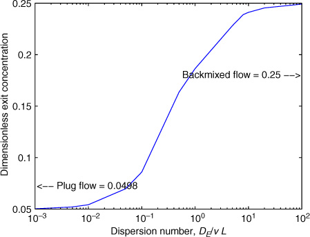
Figure 4.3 Effect of dispersion parameter on the exit concentration for a first-order reaction for Da = 3.

For a first-order reaction (and for dispersion models in general), two dimensionless parameters are needed: (1) the Damkohler number, Da, defined as k₁L/ 〈v〉; and (2) the dispersion number, defined as D_E/(〈v〉 L). The effect of the dispersion number, when keeping Da fixed at 3, is shown in Figure 4.3. The plot shows two asymptotes for low and high values of the dispersion number. For low values of dispersion number, the plug flow limit is approached. The plug flow value for Da = 3 is exp(–3) = which is 0.0498 for the exit concentration. For at high values, the backmixed result is obtained. The backmixed value is 1/(1 + Da) and is equal to 0.25. Thus the dispersion model brackets the limits of conversion that can be realized in the reactor.

4.3 Mass Exchangers

In this section we examine models for mass exchangers where mass is exchanged from one phase to another. Two cases are considered. First, we describe a single flowing stream where mass is exchanged from this stream to a second phase (which is at a fixed concentration)—for example, a transport across membrane cast as a tube. Second, we discuss two flowing phases—for example, in a gas–liquid or liquid–liquid contactor.

4.3.1 Single Stream

This section presents a simple model for transport of a solute across a porous membrane. Such a setup is common in dialysis-type devices. A mesoscopic model is quite useful to correlate the data and to predict the extent of purification that is achievable in the device. The model analyzed is shown schematically in Figure 4.4.

Diagrammatic representation of the mesoscopic model of a single stream mass exchanger.

Figure 4.4 Schematic of a single-stream mass exchanger.

Again, a bulk average concentration C_Ab is used such that the moles of A crossing any cross-sectional area (perpendicular to the flow direction) is equal to QC_Ab, where Q is the volumetric flow rate. The application of the mass balance for the solute A then leads to

\begin{matrix} Q \frac{d C_{A b}}{d z} = - (2 π R) N_{A w} & (4.17) \end{matrix}

$\begin{matrix} Q \frac{d C_{A b}}{d z} = - (2 π R) N_{A w} & (4.17) \end{matrix}$

where N_Aw is the moles of species transferred across the membrane per unit area of the walls.

A model for mass transfer across the membrane is needed, and the use of a transport law will then complete the system model. A simple law may be

N_{A w} = P_{o m} C_{A b}

$N_{A w} = P_{o m} C_{A b}$

where $P_{o m}$ $P_{o m}$ is an overall permeance parameter across the membrane. This is similar to an overall mass transfer coefficient.

In the previous equation, the driving force is the local cup mixed concentration minus the external fluid (permeate-side) concentration. We assume the external fluid concentration is zero here—an assumption that holds if the diffusing solute is collected in a large volume of liquid or is being washed away by a high flow rate of the external “sweep” fluid.

Substituting and integrating, we get the following performance equation for a single-stream mass exchanger:

\frac{C_{A b} (z)}{C_{A, i}} = exp (- \frac{2 p_{o m} z}{〈 υ 〉 R})

$\frac{C_{A b} (z)}{C_{A, i}} = exp (- \frac{2 p_{o m} z}{〈 υ 〉 R})$

This is an useful equation, for example, for determining the overall permeance value from the measured exit concentration.

Note that the permeation requires two transport steps: mass transfer from the bulk fluid to the wall, and permeation through the membrane walls. The overall permeance used in the preceding model is a combination of these two steps. It is equal to the true membrane permeance, $P_{m}$ $P_{m}$ , only if the transport to the wall from the bulk fluid is fast. This is usually the case, since the diffusion process in the membrane is much slower than that in the liquid phase. In general, a series resistance type of formula is often used:

\frac{1}{p_{o m}} = \frac{1}{p_{m}} + \frac{1}{k_{m}}

$\frac{1}{p_{o m}} = \frac{1}{p_{m}} + \frac{1}{k_{m}}$

where k_m is the mass transfer coefficient from the bulk liquid to the surface of the membrane.

4.3.2 Two Streams

Consider the modeling of the packed column absorber shown in Figure 4.5. This column is packed with some solids to promote mass transfer, with the gas and the liquid flowing (usually) countercurrent to each other.

Diagram shows the mesoscopic modeling of a packed column absorber.

A cylindrical column placed vertically is shown to have two sets of an inlet and an outlet, each at the top and the bottom. The inlets feed in from the side, while the outlets flow from the top and bottom respectively. The inlet at the top is for Liquid, L, x subscript in, while the inlet at the bottom is for Gas, G, y subscript in. The outlet at the top is for Gas, G, y subscript out while the outlet at the bottom is for Liquid, L, x subscript out. The column has a "support grid" that resembles a horizontal bar at the bottom, just above the inlet for Gas, the position of the support grid is marked z equals 0. The inlet at the top for liquid enters the column passing through a Liquid distributor that is shown to have five pipelines connected linearly. The middle portion of the column is labeled the "Packed section," which is marked with a cross across the area. The portion of the column just below the liquid distributor is marked z equals H. A sliced, horizontal portion of the column is taken as the Control Volume and its thickness is measured as delta z.

Figure 4.5 Schematic of a counterflow mass exchanger: a packed bed absorption column.

The gas and liquid phases have a common interface, and mass is transferred across the system. Each of these phases may be assumed to be in plug flow, which provides the simplest description of the mixing pattern. Alternatively, dispersion may be superimposed on the model. Also, we assume dilute systems, such that the gas flow rate does not vary significantly in the column. Constant temperature and pressure is also assumed. These assumptions allow for the simplest model for the system, which is useful for a quick design calculation. The corrections to account for these assumptions can then be applied progressively and as needed.

Based on the presence of the two phases, the control volume shown in Figure 4.6 can be set up. It consists of a gas phase and a liquid phase, with mass transfer taking place from gas to liquid. The conservation law can be applied to the gas and liquid phases.

Diagram shows a control volume for gas and liquid for a counterflow gas absorption column.

Figure 4.6 Control volume for gas and liquid for a counterflow gas absorption column.

The balance equations for the gas phase can be expressed in words:

in – out – transferred to liquid = 0

The in term is equal to G y(z), where G is the molar flow rate of the gas and y is the species mole fraction at location z. Note that y is used for y_A for simplicity of notation here.

Similarly, the out term is given by G y(z + Δz). The molar flow rate of gas is assumed to be constant—an assumption that is valid for low concentrations of the solute in the gas phase. Hence G is not a function of z. This is not true for concentrated solutes, however, and in such a case the model needs to be reformulated in terms of the mole ratio. Here we focus on dilute systems to illustrate the model building aspects.

Let the transfer rate term be denoted by ${\dot{M}}_{A}$ ${\dot{M}}_{A}$ ; this term will be modeled later in this section using a mass transfer coefficient. We will leave it as a term here to complete the first part of the modeling, the use of the conservation principle. The gas-phase balance equation in mathematical form is

G y (z) - G y (z + Δ z) - {\dot{M}}_{A} = 0

$G y (z) - G y (z + Δ z) - {\dot{M}}_{A} = 0$

Similarly, the liquid-phase balance is

in – out + transferred to liquid = 0

where in term is L x(z + Δz), The in location is now z + Δz since the liquid is flowing in the opposite direction. The out term is L x(z). The transfer term appears with a plus sign because mass is now received from the gas phase. The liquid balance is therefore

L x (z + Δ z) - L x (z) + {\dot{M}}_{A} = 0

$L x (z + Δ z) - L x (z) + {\dot{M}}_{A} = 0$

Now we close the model by writing a transport model for the ${\dot{M}}_{A}$ ${\dot{M}}_{A}$ term. When doing so, we must consider the following points.

First, we will use an overall mass transfer coefficient K_y because there are two resistances to mass transfer: from gas to interface, and from interface to bulk liquid. Details of the relation between K_y and the individual mass transfer coefficients are provided later (Section 6.5.2). For now, we simply note that K_y represents the transfer coefficient from the bulk gas phase to the bulk liquid phase. This is based on the mole fraction driving force, so the subscript y is used.

Second, the mass transfer coefficient K_y is based on the unit transfer area (intrinsic coefficient), so we multiply it by the transfer area. The latter is equal to transfer area per unit column volume, a_gl times the column volume in the differential meso-volume A_c Δz. Here A_c is the column cross-sectional area. The combined coefficient K_ya_gl is called the volumetric overall mass transfer coefficient.

The driving force must be corrected for equilibrium considerations. Note that y – x is not the driving force. The driving force is the departure from equilibrium, so y – mx is the proper driving force at any cross-section in the column. Here m is the partition coefficient, with y_eq being defined as mx. The departure from equilibrium is therefore y – mx and is the correct driving force for mass transfer.

The mass transfer rate per unit contractor volume, then, is K_ya_gl(y – mx) locally at position z. Hence the transfer rate from gas to liquid for the control volume is

{\dot{M}}_{A} = k_{y} a_{g l} (y - m x) A_{c} Δ_{z}

${\dot{M}}_{A} = k_{y} a_{g l} (y - m x) A_{c} Δ_{z}$

where A_c is the cross-sectional area of the column.

Substituting this defintion in the mass balance equations for the gas and liquid models and taking the limit as Δz tends to zero, the following equations are obtained:

\begin{matrix} G \frac{d y}{d z} = - K_{y} a_{g l} A_{c} (y - m x) & (4.18) \end{matrix}

$\begin{matrix} G \frac{d y}{d z} = - K_{y} a_{g l} A_{c} (y - m x) & (4.18) \end{matrix}$

and

\begin{matrix} L \frac{d x}{d z} = - K_{y} a_{g l} A_{c} (y - m x) & (4.19) \end{matrix}

$\begin{matrix} L \frac{d x}{d z} = - K_{y} a_{g l} A_{c} (y - m x) & (4.19) \end{matrix}$

Two endpoint conditions are required since we have two first-order differential equations and the inlet values are used as the conditions:

At z = 0, gas inlet, y = y_in

At z = L, liquid inlet, x = x_in

Solution to the Model Equations

Equation 4.19 is multiplied by m and then subtracted from Equation 4.18, which gives:

\begin{matrix} \frac{d}{d z} (y - m x) = - K_{y} a_{g l} A_{c} (\frac{1}{G} - \frac{m}{L}) (y - m x) & (4.20) \end{matrix}

$\begin{matrix} \frac{d}{d z} (y - m x) = - K_{y} a_{g l} A_{c} (\frac{1}{G} - \frac{m}{L}) (y - m x) & (4.20) \end{matrix}$

This equation can then be integrated by separation of variables if we treat (y – mx) as a variable:

\begin{matrix} \int_{i n}^{o u t} \frac{d (y - m x)}{y - m x} = - K_{y} a_{g l} (\frac{1}{G} - \frac{m}{L}) A_{c} \int_{0}^{H} d z & (4.21) \end{matrix}

$\begin{matrix} \int_{i n}^{o u t} \frac{d (y - m x)}{y - m x} = - K_{y} a_{g l} (\frac{1}{G} - \frac{m}{L}) A_{c} \int_{0}^{H} d z & (4.21) \end{matrix}$

The limits on the left are the inlet and exit values for y – mx.

The integration leads to the following equation, which relates the volume of the packed column, V_c = A_cH, to the exit mole fractions:

\begin{matrix} \begin{matrix} ln (\frac{y_{in} - {m x}_{out}}{y_{o u t} - {m x}_{i n}}) = \frac{K_{y} a_{g l}}{G} (1 - \frac{m G}{L}) V_{c} \end{matrix} & (4.22) \end{matrix}

$\begin{matrix} \begin{matrix} ln (\frac{y_{in} - {m x}_{out}}{y_{o u t} - {m x}_{i n}}) = \frac{K_{y} a_{g l}}{G} (1 - \frac{m G}{L}) V_{c} \end{matrix} & (4.22) \end{matrix}$

This expression provides one relationship between the exit mole fractions. The second relationship is obtained by using an overall mass balance.

Overall Mass Balance

The second equation relies on the invariance property of the system—that is, the overall mass balance. Equations 4.19 and 4.18 can be combined to give

\begin{matrix} G \frac{d y}{d z} = L \frac{d x}{d z} & (4.23) \end{matrix}

$\begin{matrix} G \frac{d y}{d z} = L \frac{d x}{d z} & (4.23) \end{matrix}$

The integrated form is the overall mass balance:

\begin{matrix} \begin{matrix} \begin{matrix} \begin{matrix} G (y_{i n} - y_{o u t}) = L (x_{o u t} - x_{i n}) \end{matrix} \end{matrix} \end{matrix} & (4.24) \end{matrix}

$\begin{matrix} \begin{matrix} \begin{matrix} \begin{matrix} G (y_{i n} - y_{o u t}) = L (x_{o u t} - x_{i n}) \end{matrix} \end{matrix} \end{matrix} & (4.24) \end{matrix}$

This equation is simply the statement that moles of A lost by the gas equals moles gained by the liquid.

Equations 4.24 and 4.22 permit calculation of two unknowns. Usually the inlet composition of the streams is known, which leaves three unknowns: the two exit compositions and the volume of the contacter. Two equations are available in our model, and one of the unknowns, is to be specified. Thus, if the volume of the absorber is specified, the exit mole fractions of both the gas and the liquid can be calculated (a simulation problem). Similarly, if one exit composition is specified, then the second exit concentration and the volume of the absorber needed to achieve the specified separation can be calculated (a design problem). This procedure is illustrated in Example 4.2.

Log Mean Driving Force

From Equation 4.24, we can show with a few steps of simple algebra that

\begin{matrix} (1 - \frac{m G}{L}) = \frac{[y_{i n} - {m x}_{o u t}] - [y_{o u t} - {m x}_{i n}]}{y_{i n} - y_{o u t}} & (4.25) \end{matrix}

$\begin{matrix} (1 - \frac{m G}{L}) = \frac{[y_{i n} - {m x}_{o u t}] - [y_{o u t} - {m x}_{i n}]}{y_{i n} - y_{o u t}} & (4.25) \end{matrix}$

We can replace the bracketed term on the right side of Equation 4.22 with this identity. A log mean driving force (LMDF) is now defined to simplify the final result:

LMDF = \frac{[y_{i n} - {m x}_{o u t}] - [y_{o u t} - {m x}_{i n}]}{ln ([y_{i n} - {m x}_{o u t}] / [y_{o u t} - {m x}_{i n}])}

$LMDF = \frac{[y_{i n} - {m x}_{o u t}] - [y_{o u t} - {m x}_{i n}]}{ln ([y_{i n} - {m x}_{o u t}] / [y_{o u t} - {m x}_{i n}])}$

This is the logarithmic average of the driving force at the inlet, [y_in – mx_out], and that at the outlet, [y_out – mx_in]. In turn, Equation 4.22 can be rearranged as

\begin{matrix} \begin{matrix} \begin{matrix} G (y_{i n} - y_{o u t}) = K_{y} a_{g l} (A_{c} H) \end{matrix} LMDF \end{matrix} & (4.26) \end{matrix}

$\begin{matrix} \begin{matrix} \begin{matrix} G (y_{i n} - y_{o u t}) = K_{y} a_{g l} (A_{c} H) \end{matrix} LMDF \end{matrix} & (4.26) \end{matrix}$

The left side of Equation 4.26 represents the total moles/s of gas absorbed. The right side then says that this rate is equal to the volumetric mass transfer coefficient times the volume of the absorber times a driving force that is the log mean average of the driving force at the two ends.

Equation 4.26 has an exact analogue in heat transfer for a counterflow heat exchanger:

Q = U A LMTD

where Q is the heat transferred from hot fluid to cold fluid, U is the overall heat transfer coefficient, A is the surface area of the heat exchanger, and LMTD is the log mean temperature difference.

Minimum Liquid Flow Rate

A quantity of interest is the minimum liquid flow rate. This rate can be calculated directly using the overall mass balance for A together with a thermodynamic condition. The overall mass balance is given by Equation 4.24, which is reproduced here for convenience:

G(y_in – y_out) = L(x_out – x_in)

Assume the exit liquid is in equilibrium with the inlet gas, such that x_out = y_in/m. We can then solve for L, which gives the minimum liquid flow rate to be used.

If the entering liquid is fresh, then x_in = 0 and we get the following expression for the minimum liquid flow rate:

\begin{matrix} L_{\min} = m G \frac{(y_{i n} - y_{o u t})}{y_{i n}} & (4.27) \end{matrix}

$\begin{matrix} L_{\min} = m G \frac{(y_{i n} - y_{o u t})}{y_{i n}} & (4.27) \end{matrix}$

Figure 4.7 shows the concept of the minimum liquid flow rate needed. The operating line touches the equilibrium line at the conditions of minimum L/G, known as the pinch point.

Graphical representation of the Gas absorption column design problem.

The horizontal axis represents Mole fraction in liquid denoted by variable x and the vertical axis represents Mole fraction in vapor denoted by variable y. Graph legend reads P equals (y subscript in by m, y subscript in): Pinch, B equals (x subscript out, y subscript in): Bottom, and T equals (x subscript in, y subscript out): Top. A linear line diagonal to the quadrant is drawn from the origin. This line is labeled "Equilibrium line, y superscript asterisk equals m times x. Two other lines with positive slopes, one dashed and one solid is shown to originate at point T, the solid line above the dashed line. The dashed line tends to meet the equilibrium line at point P at the end of the line. This line is labeled Minimum L by G line. The solid line moves upward and stops at point B and is labeled Operating line, slope equals L by G.

Figure 4.7 Gas absorption problem shown as a plot of operating line and equilibrium curve.

Typically the liquid flow rate is 1.4 times the minimum. This provides all the key information needed to design a two-phase mass exchanger based on the assumption that both phases are in plug flow and they flow countercurrent to each other. The calculations are illustrated in Example 4.2.

Example 4.2 Gas Absorption Column Design

A solute A is to be recovered from a gas stream, and the following conditions are specified: The gas flow rate is 0.062 kmol/s with 1.6% solute; the liquid flow rate is 1.4 times the minimum and the solubility coefficient, m, is 40.

The column should provide an outlet mole fraction of 0.004. Find the height of the absorber.

Use a value for the overall mass transfer coefficient of 0.05 kmol/m³ s per mole fraction difference. Usually this value depends on the operating gas and liquid velocities and the type of packing used, and is estimated using empirical correlations.

Solution

We have y_in = 0.016 and y_out = 0.004. Also x_in = 0 since a pure liquid is being used.

The minimum liquid flow rate can be computed using Equation 4.27:

L_min = 40 * 0.062 * (0.0166 – 0.004)/0.016 = 1.86 kmol/s

The value of L is usually 1.4 times the minimum flow. Hence L = 2.6 kmol/sec.

The mole fraction in the liquid exit is calculated using Equation 4.24. It gives x_out as 2.86 × 10^–04.

Now we can find the log mean driving force. The driving force at the gas inlet is y_in – mx_out = 0.0046. The driving force at the gas outlet is y_out – mx_in = 0.004 0.043. The logarithmic average of the two is calculated as (0.0046 – 0.004)/ln(0.0046/0.004) and is equal to 0.0043.

The volume of the column needed can then be calculated using Equation 4.26. The required volume is found to be 3.4772 m³.

Column diameter is chosen based on flooding considerations, which will depend on the operating velocity. Too high a velocity will cause flooding in the column, so that the liquid will not find its way down. Too low a velocity will result in poor mass transfer. We will use an operating gas velocity of 1 m/s here for illustration. The gas volumetric flow rate is calculated as 1.5 m³/s, so the column’s cross-sectional area is 1.5 m². The column diameter is therefore equal to 1.2 m and the height of the column needed is 2.31 m.

4.3.3 NTU and HTU Representation

The design equations can also be cast in an alternative form, known as the NTU, HTU representation. The gas-phase balance (Equation 4.18; repeated here) is the starting point for developing the HTU and NTU representation:

G \frac{d y}{d z} = - k_{y} a_{g l} A_{c} (y - m x)

$G \frac{d y}{d z} = - k_{y} a_{g l} A_{c} (y - m x)$

Using y* for mx, this can be generalized as

\begin{matrix} G \frac{d y}{d z} = - K_{y} a_{g l} A_{c} (y - y *) & (4.28) \end{matrix}

$\begin{matrix} G \frac{d y}{d z} = - K_{y} a_{g l} A_{c} (y - y *) & (4.28) \end{matrix}$

This form is applicable even to the nonlinear equilibrium relationship y* = y*(x), where x is the local liquid mole fraction and y* is the corresponding equilibrium value.

Equation 4.28 can be rearranged to

\begin{matrix} H = [\frac{G}{K_{y} a_{g l} A_{c}}] [\int_{i n}^{o u t} \frac{d y}{y - y *}] & (4.29) \end{matrix}

$\begin{matrix} H = [\frac{G}{K_{y} a_{g l} A_{c}}] [\int_{i n}^{o u t} \frac{d y}{y - y *}] & (4.29) \end{matrix}$

The first bracketed term is called HTU (height of transfer unit), while the second term is called NTU (number of transfer unit).

HTU = \frac{G / A_{c}}{K_{y} a_{g l}}

$HTU = \frac{G / A_{c}}{K_{y} a_{g l}}$

where G/A_c is molar superficial gas velocity, in mol/m²s. The HTU parameter has the units of height and represents the ease or difficulty of mass transfer. Larger values indicate poorer mass transfer. Data are available for a wide range of packing materials used in practice. The range of values is from 0.3 to 1.1 m.

The integral term in Equation 4.29 is referred to NTU:

NTU = \int_{i n}^{o u t} \frac{d y}{y - y *}

$NTU = \int_{i n}^{o u t} \frac{d y}{y - y *}$

It is measure of the driving force available for mass transfer.

Hence the height of the column required is calculated as the product of HTU and NTU:

Height of column = HTU × NTU

This form can be used for both linear and nonlinear equilibria. The only restriction is that it is valid just for dilute systems—that is, when the gas velocity does not change significantly in the column. The NTU must be evaluated from numerical integration for the nonlinear case, whereas analytical solutions can be found for the linear case as shown in Example 4.3. Since the gas-phase mole fraction was used to define the driving force and mass transfer coefficients, Seader et al. designate HTU as H_OG and NTU as N_OG. Other definitions, such as H_OL and N_OL, can also be used. These definitions apply when the liquid mass balance is used as the starting point instead of Equation 4.28. The final results for the height of the column will be unchanged.

For linear systems, the value of NTU can be obtained analytically as shown in Example 4.3.

Example 4.3 NTU Equation for a Linear Equilibrium Case

Derive an expression for NTU for a linear equilibrium relation, and apply it to Example 4.2.

Solution

For a linear relation, y* = mx and the integral for NTU is:

\begin{matrix} N T U = \int_{y i n}^{y o u t} \frac{d y}{y - m x} & (4.30) \end{matrix}

$\begin{matrix} N T U = \int_{y i n}^{y o u t} \frac{d y}{y - m x} & (4.30) \end{matrix}$

At any point in the column, x is related to y by

L(x – x_in) = G(y – y_out)

which is the mass balance from the top of the column to any arbitrary height. Thus,

x = x_{i n} + \frac{G}{L} (y - y_{o u t})

$x = x_{i n} + \frac{G}{L} (y - y_{o u t})$

If this definition is substituted into Equation 4.30, the integration can be performed analytically. The final result for the common case of x_in = 0 is

N T U = (\frac{1}{1 - m G / L}) ln [\frac{y_{i n} (1 - m G / L) + y_{o u t} m G / L}{y_{o u t}}]

$N T U = (\frac{1}{1 - m G / L}) ln [\frac{y_{i n} (1 - m G / L) + y_{o u t} m G / L}{y_{o u t}}]$

For Example 4.2, the parameter mG/L is calculated as (40 * 0.062/2.6) = 0.9524. Now we can substitute the inlet and exit concentrations and this parameter and estimate the NTU as 2.804.

The HTU is calculated as (0.062/1.5)/0.05 = 0.8267 m. The column height is the product of the NTU and the HTU and is equal to 2.318 m.

Summary

Mesoscopic models are useful if there is a principal direction of flow along which the concentration changes significantly. Examples include a pipe flow reactor and a packed bed exchanger. The concentration variation in the cross-flow direction is not modeled; instead, its effect is captured by cross-sectional averaging. Thus the control volume spans a differential length in the flow direction and the entire pipe or reactor cross-section in the cross-flow direction.
Two types of average concentrations can be defined: the flow weighted or the cup mixed average and the cross-sectional average. Their definitions are important to understand.
The mass transfer coefficient concept is needed for meso-modeling applications, since the local wall flux value is not available. The coefficients are often calculated using empirical correlations. The cup mixed concentration is used as a measure of the fluid concentration in defining the driving force for mass transfer in pipe or channel flows.
Solid dissolution from a pipe wall is the simplest problem in mesoscopic modeling. All the steps that go into the model formulation were shown in detail in this chapter, and form the basic pattern for mesoscopic modeling. An average mass transfer coefficient over the entire length of the pipe is used in these models since the local values can vary as a function of axial position.
Mass transfer data can be correlated using dimensionless parameters, and such correlations are readily available for a large number of problems, including pipe flow. Commonly, a dimensionless parameter, the Sherwood number, is used as a dimensionless mass transfer coefficient. It is correlated in terms of the Reynolds and Schmidt numbers. The product of the Reynolds and Schmidt numbers is known as the Peclet number.
Tubular flow reactors are often modeled using the concept of plug flow at a first level of approximation. The effect of non-uniform velocity is ignored in this model. The cup mixing and cross-sectional averages are the same here and no additional closure is needed.
The dispersion model is an attempt to correct for the deviation from plug flow. The dispersion coefficient D_E is used as a parameter here. The value of D_E is zero for a plug flow case; in contrast, the value is close to infinity for a completely backmixed system.
The dispersion coefficient should not be confused with the diffusion coefficient, although the units are the same for both (m²/s.)
Mass transfer units with one or two flowing phases can be modeled using mesoscopic models. The phases may be assumed to be in plug flow for a simple model. Often the dispersion concept is superposed on plug flow to account for the deviations from the ideal contacting pattern of plug flow.
Mass transfer in a countercurrent mass exchanger is a well-studied problem and has many applications in the design of absorption and extraction processes and similar operations. This problem has an analogy with heat exchangers. The concept of log mean driving force provides a relation for the volume of the contactor required to achieve a given degree of separation.

Review Questions

4.1 Define cup mixing and cross-sectional average concentration.

4.2 How is the driving force defined for mass transfer in pipe flow?

4.3 Distinguish between local and average mass transfer coefficients.

4.4 What is the plug flow assumption and why is it useful?

4.5 Which parameter is commonly used to correct the deviation from plug flow?

4.6 When is the plug flow assumption inadequate?

4.7 Write the formula to calculate the dispersion coefficient for a pipe flow of Newtonian fluid.

4.8 Explain why the dispersion coefficient is inversely proportional to the diffusion coefficient.

4.9 What is the definition of the dispersion Peclet number?

4.10 Is plug flow approached for low or high values of the dispersion Peclet number?

4.11 Define logarithmic mean driving force for two-phase mass transfer.

4.12 What is meant by the pinch point?

4.13 How is the minimum liquid flow rate calculated in an absorption column?

4.14 Define HTU and NTU, and state the equation used to find the height of a countercurrent mass exchanger.

Problems

4.1 Mass transfer coefficient calculations in pipe flow. Calculate and plot the average mass transfer coefficient from bulk to pipe wall as a function of position from the entrance of the pipe for the following conditions. The pipe diameter is 1 cm.

– Flow is laminar with a Reynolds number of 1000. Carrier fluid is air with D_A = 2 × 10^–4 m²/s.

– Flow is laminar with a Reynolds number of 1000. Carrier fluid is water with D_A = 2 × 10^–9 m²/s.

– Flow is turbulent with a Reynolds number of 5000. Carrier fluid is air with D_A = 2 × 10^–4 m²/s.

– Flow is turbulent with a Reynolds number of 5000. Carrier fluid is water with D_A = 2 × 10^–9 m²/s.

4.2 Lead contamination in a corroding pipe. A pipe has a diameter of 2.5 cm and a lead soldered section that is 15 cm long. The water flows in the pipe with an average velocity of 0.2 m/s. The saturation solubility of lead compound is 10 g/m³. Find the dissolved lead concentration at the pipe exit if the mass transfer coefficient for solid dissolution has a value of 2 × 10^–5 m/s.

4.3 Microchannel reactor with a wall reaction. A microchannel reactor consists of two parallel plates spaced 3 mm apart and 1 m wide. Gas at a flow rate of 0.05 m³/s containing a pollutant flows in the gap between the two plates. The wall are coated with a catalyst, and a surface reaction is taking place on the pipe wall. Assume the surface reaction to be fast. Calculate the length of the channel required to remove 90% of the pollutant. Use 7.54 as the value of the average Sherwood number. Note that this is defined as k_md_h/D_A, where d_h is the hydraulic diameter.

4.4 Mass transfer value from measured absorption data. Ammonia (5%) from air is absorbed into water falling as a thin film of liquid over a vertical wall of height 1 m. The flow rate of water is 5 × 10^–3 kg/s per unit width of the plate. The thickness of the film is 1.4 × 10^–4 m. The exit concentration of ammonia in the liquid is 200 mol/m³ and the Henry’s law coefficient is 30 atm. What is the value of the mass transfer coefficient in this system? Assume gas is in excess.

4.5 Comparison of plug flow and backimixed flow reactors. Show that the steady state exit concentration for a first-order reaction is 1/[1 + Da] for a backmixed flow. Determine the corresponding expression if the reactor is modeled as a plug flow reactor. Make a comparison plot of the exit concentration for these two cases as a function of Da. Show that if Da < ≈ 0.3, then the mixing behavior is not important and the two models give nearly the same conversion.

4.6 Second-order reaction in plug flow. Derive an expression for the exit concentration for a second-order reaction taking place in a plug flow reactor.

4.7 Zero-order reaction in plug flow. A zero-order reaction with a rate constant of k₀ is carried out in the plug flow reactor. Show that the dimensionless exit concentration is given as

c_A,e = 1 – Da for Da ≤ 1

where Da is defined as

D a = \frac{V k_{0}}{Q C_{A, i}}

$D a = \frac{V k_{0}}{Q C_{A, i}}$

Find the exit concentration if Da is greater than 1.

4.8 Bimolecular reaction in a pipe. An aqueous feed to a pipe flow reactor consists of a mixture of A and B with concentrations of 100 mol/m³ and 200 mol/m³ for A and B, respectively. The feed flow rate is 0.04 m³/s, and the following reaction takes places as:

A + B → products

The rate of reaction (S.I. units) follows bimolecular kinetics:

R_A = 0.4C_AC_B

Find the exit concentration of A and B if the reactor volume is 1 L. Assume plug flow.

4.9 Membrane aeration system. Membrane aeration systems are used in some applications to transfer oxygen to water or other liquids. They have applications in biomedical engineering. Such a system consists of an inner tube, with water containing no dissolved oxygen entering the system. The inner tube is surrounded by an annular tube, with a permeable wall separating the two tubes. Pure oxygen at a pressure of 2 atm is maintained in the annular tube. A 35% oxygen saturation was observed for a tube of 40 m for an average velocity of water of 50 cm/s. The inner tube diameter is 1 cm.

Determine the overall membrane permeance. Also calculate the mass transfer coefficient in the system and use the series resistance formula to find the true membrane permeance.

4.10 Height of an absorption column: LMDF method. A gas stream containing 8 mol % of ammonia is to be purified to an exit concentration of 0.5 mol % ammonia. The gas’s superficial molar velocity is 100 kg mol/h m². Water is used as the absorbent, with the flow rate being 1.5 times the minimum flow rate. The mass transfer coefficient K_ya_gl is estimated as 0.2 kg mol/h m³. Use a constant value of 1 for the solubility parameter, m—although the equilibrium for ammonia–water is actually nonlinear. Find the height of the column needed using the log mean driving force method.

4.11 Height of an absorption column: NTU-HTU method. For problem 10, find NTU and HTU parameters and calculate the height of column again.

4.12 Simulation with MATLAB BVP4C solver. Numerical solutions of Equations 4.18 and 4.19 are examined in this problem. Write these equations in dimensionless form by introducing a dimensionless length ζ = z/H. Show that the two dimensionless parameters defined here are needed. First is the dimensionless mass transfer parameter:

\begin{matrix} k_{g l} = \frac{K_{y} a_{g l} H}{G} & (4.31) \end{matrix}

$\begin{matrix} k_{g l} = \frac{K_{y} a_{g l} H}{G} & (4.31) \end{matrix}$

where $G$ $G$ is the molar velocity, G/A_c. Second is the flow ratio parameter, G/L.

Show that the model equations now take the following simple forms:

\begin{matrix} \frac{d y}{d ζ} = - α_{g l} (y - m x) & (4.32) \end{matrix}

$\begin{matrix} \frac{d y}{d ζ} = - α_{g l} (y - m x) & (4.32) \end{matrix}$

and

\begin{matrix} L \frac{d x}{d ζ} = - α_{g l} \frac{G}{L} (y - m x) & (4.33) \end{matrix}

$\begin{matrix} L \frac{d x}{d ζ} = - α_{g l} \frac{G}{L} (y - m x) & (4.33) \end{matrix}$

Boundary conditions are needed at the two endpoints of ζ of 0 and 1. State the conditions. Write code to simulate this system using the MATLAB BVP4C solver. Use the code to model an absorber for the following conditions:

– Gas flow rate, G = 0.062 mol/s with a solute mole fraction of 1.6%

– Liquid flow rate, L = 1.6 mol/s with no dissolved solute

– Column area = 1.5 m²

– Solubility coefficient, m = 40

– Overall mass transfer coefficient, K_ya_gl = 0.05 mol/m³ s

– Height of the absorber, H = 2.3 m

Plot the liquid and gas mole fractions as a function of column height.

..................Content has been hidden....................

You can't read the all page of ebook, please click here login for view all page.

Table of Contents for Chapter 4. Examples of Mesoscopic Models

Create new playlist

Sign In

Sign Up

Chapter 4. Examples of Mesoscopic Models

4.1 Solid Dissolution from a Wall

4.1.1 Model Details

4.1.2 Mass Transfer Correlations in Pipe Flow

4.2 Tubular Flow Reactor

4.2.1 Plug Flow Closure

4.2.2 Dispersion Closure

Dispersion Coefficient in Laminar Pipe Flow

Effect of Dispersion

4.3 Mass Exchangers

4.3.1 Single Stream

4.3.2 Two Streams

Solution to the Model Equations

Overall Mass Balance

Log Mean Driving Force

Minimum Liquid Flow Rate

4.3.3 NTU and HTU Representation

Summary

Review Questions

Problems

Table of Contents for
Chapter 4. Examples of Mesoscopic Models