Chapter 22. Reactive Membranes and Facilitated Transport

This chapter analyzes the transport across a membrane containing a reacting species known as the carrier. The following reaction scheme is illustrative of many common cases:

In this scheme, species A, the diffusing solute, reacts with B to form a complex C and is transported in both the free (A) and combined forms (C). An important example is hemoglobin in blood RBC (red blood cells) and myoglobin in tissues, which binds strongly to oxygen, By itself the oxygen solubility in blood is small and life as we know it for human beings cannot be sustained by this small solubility. Here is where the hemoglobin comes into action. Oxygen is carried in free and combined forms and is desorbed by the reverse reaction to provide adequate oxygen concentration for metabolism in the tissues.

In industrial practice there are various ways of immobilizing a carrier, as shown in Section 22.3; the system then acts as a reactive membrane. Higher fluxes can be obtained in these systems than possible if there were no reaction in the membrane. In some cases very selective separation is also possible. The process is also known as facilitated diffusion since the carrier enhances the transport of A.

The system exhibits a number of complexities compared to ordinary diffusion and these are primarily due to the simultaneous reaction taking place. One of the goals in this chapter is therefore to demonstrate the application of the diffusion-reaction model to calculate the enhancement on the transport of A due to the above complex formation.

Maximum enhancement is obtained when the reaction given in Equation 22.1 is fast relative to diffusion. This is known as the instantaneous reaction regime and is more commonly encountered in practice. An asymptotic solution can be obtained for this case similar to that for an instantaneous reaction in gas–liquid systems. The kinetics of reaction plays no part in the model for such cases. Some parametric dependency of the flux on the concentration gradient and the equilibrium constant will be shown in this chapter based on the analytical solution for this case.

Facilitated diffusion with more than one solute diffusing across the system can have many complex features. The two solutes can compete for the same carrier; this is sometimes referred to as counter-transport. The rate of transport of one solute can be curtailed by the other solute and can even occur counter to its own gradient.

In some cases the second solute can bind together to the same carrier along with the first solute; this is referred to as co-transport. The presence of the second solute can then enhance the transport of the first solute. In some cases the first solute can be transported even when its concentration gradient is zero. These effects are indicated.

A general model for reactive membranes in which multiple equilibrium reactions are taking place is then shown and implemented in MATLAB. This can be used to simulate membrane systems with complex chemistry including counter- and co-transport and is a useful tool to examine parametric effects and to fit experimental data for such reactive membranes.

The chapter concludes with some discussion on industrial applications of reactive membranes. The discussion is brief but some useful references are provided as a starting point for further study of this topic.

Here A is the species being transported across a membrane of thickness L while B and C are the free and the bound carrier. These stay within the membrane. Species A is thus transported in free form as well as bound form as C from one side to the other side of the membrane. The model to compute the flux of A across the membrane is presented in the following section.

Here k₂ is the rate constant for the forward reaction and K is the equilibrium constant.

Boundary conditions are set as follows:

For species A we can specify the concentration at the two sides of the membrane C_A(x = 0) = C_A0 and C_A(x = L) = C_AL. Note that these are concentrations in the membrane phase and not in the external fluid near these sides. If the external concentrations are known, then the membrane phase concentrations have to be obtained by multiplying the external concentrations by the partition coefficient. Thus for example, C_A0 = K_pAC_A0,f, where K_pA is the solubility coefficient of A in the membrane and C_A0,f is the concentration in the fluid phase adjacent to the membrane.

Species B and C are bound to the carrier and hence they cannot diffuse out the membrane. Hence the no flux conditions are used for both these species at both x = 0 and x = L. Since no flux is specified at both sides, there is no base concentration to calculate the concentration profiles and the flux of A. Hence the problem is not uniquely specified. We have to augment the problem by an integral condition that states that the total concentration of B in free form and bound form is fixed and equal to some value C_BT, the total concentration of B+C in the membrane. This leads to the following integral constraint on the concentrations of B and C:

Once C_BT is specified by the above integral constraint, the problem has a unique solution. This equation is simply a mass balance for the total carrier concentration within the membrane.

The set of dimensionless equations are as follows:

and

Note that in the above representation we have used D_C = D_B, that is, equal diffusivity for the free and bound carrier, for simplicity. The values would generally be close to each other. Also note the similarity in the model to the gas–liquid reactions discussed in Chapter 20. The integral constraint on B is the only additional modeling feature to be added here.

The dimensionless parameters needed in the model are as follows:

• A Hatta type of modulus parameter representing the ratio of the diffusion time to the reaction time:

  M² = k₂C_BT (L²/D_A)

• A parameter that is the measure of the relative concentrations of B and A and their diffusivity values:

  q=DBCBTDACA0

• Dimensionless equilibrium constant:

  K* = KC_A0

Thus the performance of the system is characterized by three dimensionless parameters, M, q, and K*.

Results are often presented in terms of the enhancement factor, which is defined as –dc_A/dξ calculated at the surface. For no carrier this will be equal to one and hence this factor shows the augmentation of transport due to the presence of the carrier. An illustrative solution to the model is presented in terms of the key dimensionless parameters in Figure 22.1.

This is for large M of 1000 and was generated using BVP4C. Note that the concentration of all three species changes significantly within the membrane. The enhancement factor is simply the negative of the slope of A in dimensionless concentration. It shows to what extent the faciliated diffusion enhances the rate of transport of A. The value for the given set of parameters was found to 4.33.

We now study two asymptotic features of the solution: the large M case where the reaction is treated as instantaneous and the small M case where a pseudo-first-order approximation can be made. Before we proceed it may be in order to look at the invariant of the system.

Integrating twice and using the total constraint condition given by Equation 22.5 (in dimensionless form) yields:

This is nothing but a restatement of the combined mass balance for the total carrier, that is, c_C + c_B must be one. The carrier must be either in free or combined form since it cannot escape the membrane. The model equations can be reduced from three to two now by eliminating, say, c_C from the rate terms in Equations 22.6 and 22.7.

Combining Equations 22.6 and 22.8 we find

d2cAdξ2+qd2cCdξ2=0

Integrating once we find that the total flux of species A is

The constant p₀ is the gradient of A at the surface and hence dimensionless flux of A diffusing across the membrane is equal to –p₀. A second integration gives an invariant relation:

Here A₂ is the second integration constant. If Equation 22.12 is applied at ξ = 0 we have

c_A(0) + qc_c(0) = A₂

If Equation 22.12 is applied at ξ = 1 we have

c_A(1) + qc_c(1) = p₀ + A₂

Combining these the expression for the dimensionless flux can be obtained and related to the end point values of the concentration:

Further simplification can be made by using the equilibrium assumption c_C = K*c_Ac_B and the total balance on the substrate c_B = 1 – c_C. These conditions lead to

cc=K*cA1+K*cA

This can be used at the two ends of the membrane to find c_C(0) and c_C(1). Also we use c_A(0) = 1. Substituting all this in the expression for combined flux in Equation 22.13 we find

In the more common case of c_A(1) =0 (the receiving end is at zero concentration of the solute) this simplifies to

Dimensionless flux of A=1+qK*1+K*

The flux in terms of dimensional variables is

This can be used to illustrate some parametric features of the system. The first term is the ordinary diffusion, also called the passive diffusion, and is the flux in the absence of the carrier. The second term on the right-hand side can be viewed as the enhancement in transport due to the presence of a the reacting carrier for the case of a rapid reaction asymptote. This is the contribution of the facilitated transport.

Additional features are discussed in the following paragraphs.

The flux depends now on the diffusive transport of the carrier from one side to the other side of the membrane. Also the equation shows that the 1/N_A0 versus 1/C_A0 plot should be linear, which can be used to fit the experimental data.

The rate of transport depends on how fast B can move from one side to the other. The extent of binding of A with the carrier makes no difference now. The explanation is that species A binds so strongly to the carrier that no reverse reaction takes place at the other end to release back the solute. This has important implications in choosing the carrier. It should not bind very strongly to the solute. The equilibrium of the solute–carrier complexation must provide a delicate balance. The forward complexation rate must be sufficiently high to obtain a large amount of complex and hence, a high enhancement effect. On the other hand, the reverse rate must also be large enough to readily reverse the complexation step at the receiving end so that the solute can be recovered and the carrier diffused back to pick up more solute from the feed end.

The concentration of the substrate and the complex is observed to be nearly constant in this case and the model can be simplified by using a constant concentration of B and C in the membrane. Hence the differential equation for A reduces to a linear equation and the solution can be derived analytically for this case. The details are not shown here but exercise problem 22.5 addresses some of these calculations. In general the enhancement factors for the fast diffusion case are lower than the fast reaction case. Hence one should seek carriers with fast reactions so that the maximum benefit of binding with the carrier can be obtained.

The results of a parametric study of varying the M parameter are shown in Table 22.1.

Table 22.1 Effect of M Parameter on the Enhancement Factor for Solute Transport across a Reactive Membrane for q = 5 and K* = 2

M	1	10	100	1000	10,000	∞
E	1.04	2.72	3.92	4.28	4.32	4.33

The results in this table confirm the discussion that at low M the enhancement factor is low and is nearly equal to one. It also shows that as M increases the enhancement factor approaches the instantaneous reaction asymptotic value.

Solute 1 + Substrate S ⇌ Complex S+1

Solute 2 + Substrate S ⇌ Complex S+2

Solutes 1 and 2 can both diffuse in and out of the membrane while the substrate, complex 1, and complex 2 cannot leave the membrane. Under certain conditions, species 1 (or 2) can be transported against its own concentration gradient. Hence the phenomena is known as counter-transport. Examples are common in biological systems. Thus oxygen and CO can both bind with hemoglobin, leading to counter-transport of oxygen and CO poisoning. On a similar note the cure for methanol poisoning is ethanol, which displaces methanol from the liver enzyme. Additional examples of counter-transport are shown by Cussler (2009) and Noble and Koval (2005).

Co-transport occurs when the following type of overall reaction scheme holds:

Solute 1 + Solute 2 + Substrate S ⇌ Complex S+1+2

In this case solute 1 can be transported by solute 2 or vice versa. Transport of solute 1 can occur even if there is no concentration gradient or even against its own concentration gradient. Thus solute 1 can carry solute 2 along with it and hence the phenomena is known as co-transport.

An in vitro example would be a combination of an anion (solute 1), a cation (solute 2), and a membrane with some amine as a carrier (substrate). Additional in vivo examples can be found in biological systems as indicated by Cussler (2009).

Co-transport can enhance the transport of one solute due to it being carried by the second solute. An example is presented by Caracciolo et al. (1975) where sodium ions are moved even when the concentration gradient is zero due to co-transport with Li ions. This has important applications in metal recovery and wastewater treatment, especially for the dilute metal solution commonly encountered in hydrometallurgy.

Detailed analysis of both counter- and co-transport can be done by setting up the differential models for each of the species, identifying the dimensionless groups, and computing the results. If the reactions can be assumed to be fast then the equilibrium assumption for each of the reactions can be invoked, leading to analytical solutions. Models are now presented in Sections 22.2.1 and 22.2.2 followed by a general model in Section 22.3 for fast multiple reactions where all the reactions are assumed to be in equilibrium.

The equations for species A and C are the same as those in section 22.1.1 while that for B is modified by adding an extra term for reaction with P:

Here K_A and K_P are the equilibrium constants for the two reactions. The small ks are the two rate constants.

Two additional equations for P and E are to be added. These are presented as the following pair of equations:

The equations can be solved numerically although it represents a stiff set of differential equations, especially for large values of the Hatta parameters.

The equilibrium approach is presented in further detail in the following.

Flux of A=NA0=NAL=DAŁ(CA0−CAL)+DCL(CC0−CCL)

The formal proof of this is similar to that for single instantaneous reaction discussed in Section 22.1.4.

The concentration of C at the two ends is now determined by stoichiometry and the equilibrium consideration. First we need an expression for the concentration of unreacted carrier B. This is an invariant of the system and represents the fact that the carrier B must exist as free, combined as C, or combined as E. The resulting expression can be shown to be

This can be then used in the equilibrium condition applied at the two edges of the membrane. For example at x = 0, C_C(0) = K_AC_A0C_B0. Hence

CC(0)=KACBTCA0(1+KACA0+KPCP0)

A similar equation holds for C_E0 and at the other end x = L as well for both C and E.

The final result for the flux for the common case where the receiving end is at zero concentration, that is, C_AL = 0, is

NA0=NAL=DLCA0(1+F)

where F is the enhancement or facilitation factor, which now includes the interaction of the solute P . This is given by

F=KACBT(1+KACA0+KPCP0)

A similar equation holds for the flux of P . These models are based on equal diffusion coefficients for all the species. The analysis can be modified for variable diffusivity in a similar manner.

A + B + S ⇌ C

where S is the carrier and C is a complex of A, B, and S. The result of the equilibrium model can be derived as

Note that the product of the concentrations of A and B now appears in the facilitation term.

The diffusion-reaction equation for species j is written in general form as

Djd2Cjdx2=∑iνi,jRi

where ν_i,j is the stoichiometric coefficient for species j in the ith reaction. The equation can be formally integrated once from 0 to x to give

where N_j0 = –D_j(dC_j/dx)_x=0, the flux of A at the surface. Here s is a dummy variable for integration. This flux term is set to zero for all the species that do not leave the membrane and is retained only for the solutes that cross the membrane.

A second formal integration of Equation 22.24 from 0 to L provides a relation between the concentration of species j at x = 0 and x = L:

Cj0−CjL=1Dj∑iνi,jQi−NAjLDj

Q_i results from the second integration and is obainted as the following constant, one for each reaction:

Qi=∫0L(∫0xRi(s)ds)dx

Each reaction provides an integral of this form corresponding to its rate function. These integral constants can be viewed as the tie or mapping between the end point concentrations. They are evaluated by applying the equilibrium relations.

Now the equilibrium constraints are used at the two ends. This generates an additional 2 * nr equations, which completes the set of equations. Here nr is the total number of independent reactions (for example 2 for the counter-transport considered in Section 22.2.1). An additional constraint is the total balance equation for the carrier. This completes the set of equations needed to execute the computations. The concentration relations, equilibrium relation, and the total balance constrains are solved together as a set of algebraic equations. The computer program to do this is presented in Listing 22.1.

---

Listing 22.1 Simulation of Facilitated Transport of General Network of Equilibrium Reactions

Click here to view code image

% counter–transport membrane simulation
function nonlinear
global nu K1 K2 bTotal a0 a1 p0 p1
% stoichiometry
%%%   A  P  B  C  E
nu = [ –1 0 –1 1 0;
        0 –1 –1 0 1];
  K1 = 5; K2=50;
  a0= 1; a1= 0.0;
  p0 = 0.20 ; p1=0.00;
  bTotal = 5
y0 = [ 1 1 1 1 2 1 1 1 1 1 ];
       y = fsolve(@myfun, y0)
       fluxA = y(9)
       fluxB = y(10)
  %%%%%%%%%%%%%%%%%%%%%%%%%%%%%%%%%%%%
   function F = myfun(y)
       global nu K1 K2 bTotal a0 a1 p0 p1
% unwrap the variables
b0 = y(1); b1= y(2); c0 = y(3);
c1= y(4); e0 = y(5); e1=y(6);
Q1= y(7); Q2 = y(8); fluxa = y(9); fluxp = y(10);
% set up equations
% 1 to 5 concentration tie–ups
F(1) = a0–a1 + nu(1,1)*Q1 – fluxa  ; % A
F(2) = p0–p1 + nu(2,2)*Q2 – fluxp  ; % A
F(3) = b0–b1+nu(1,3)* Q1 + nu(2,3)*Q2 ; % species B
F (4) = c0–c1+nu(1,4)* Q1 % c;
F(5) = e0–e1+nu(2,5)* Q2 ;
F(6) = b0+c0+e0 –bTotal % balance constraint
% equlibrium relations
F(7) = c0–K1*b0*a0;
F(8) = e0–K2*b0*p0;
F(9) = c1–K1*b1*a1;
F(10) = e1–K2*b1*p1;

---

For the counter-transport discussed, the unknowns are the concentrations of B, C, and E at the two end points of the membrane (total of six), the two tie parameters Q₁ and Q₂, and the flux of the solutes A and P across the membrane. Thus there are ten unknowns. Ten algebraic equations are available and can be set up and solved with FSOLVE. Upon running the program for the parameters, the following result is obtained for the fluxes of A and B:

N_A = 2.5625 and N_P = 3.3250. Scaled units are used here.

You may wish to verify that these are also consistent with the analytical solution presented earlier.

If the equilibrium constant for the second reaction is set to zero, the following results are obtained:

N_A = 5.1667 and N_P = 0.2. Scaled units are used here.

Here the passive diffusion value for flux is obtained for P since K_P = 0 and the single solute value is obtained for A.

Comparing the two cases shown previously, we find the presence of P, although in a smaller concentration (one fifth of A), has caused a significant drop in flux of A for the first case because the equilibrium constant for P (50) is much larger than that for A (5). The poisoning effect of the strongly complexing solute is illustrated here.

N_A = –2.6042 and N_P = 3.3250. Scaled units are used here.

The flux of A is now negative although its concentration gradient is zero. The solute P complexes strongly with B and the equilibrium for C shifts to the left, releasing A at x = 0.

An example of osmotic diffusion is NaCl transport in membranes with crown ethers as a carrier. This was studied by Caracciolo et al. (1975). Here one side of the membrane was maintained at 1 M NaCl and 1 M LiCl. The other side was 1 M NaCl and no LiCl. The LiCl was assumed to be a passive diffuser merely providing extra chloride ions so that electroneutrality was not violated. The sodium ion was found to diffuse against its own concentration gradient until a certain level of concentration difference was achieved. The complex of Na ion, Li ion, and the crown ether was responsible for this osmotic diffusion phenomena. For more details and experimental data on this system, please refer to the preceding reference. The program in Listing 22.1 can be adapted and used to model this and similar systems.

• There should be no side reactions that will lower the transport of A.

• The carrier must stay in the membrane phase and should not be leached out from it.

• The carrier must remain as a solid solution in the membrane phase and must not form a precipitate or some related phase change within the membrane.

• The reaction between the carrier and the solute should be relatively fast.

• The equilibrium constant must be within an intermediate range. A value that is too low does not provide enough enhancement. Too high a value causes an irreversible binding with the result that the solute does not get released at the lean end of the membrane.

Several configurations of membranes have been developed, each with its own domain of application. Some common ones are briefly discussed in the following.

The advantages are creation of a large surface to volume ratio for mass transfer. Difficulties are associated with emulsion stability and the process of de-emulsification to recover the receiving phase.

ELM has been applied for recovery of metals from lean leach solution. An example is the extraction of nickel using D2EHPA (di-2ethyl-hexyl phosphoric acid) as a carrier, studied by Kulkarni et al. (1999). The reaction scheme is an exchange of a nickel ion for two hydrogen ions:

Ni⁺⁺ + 2RH → NiR₂ + 2H⁺

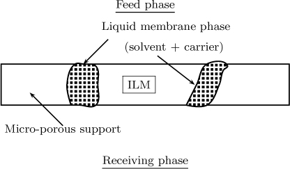
CO₂ in amine solution is an example of ILM and the work of Marzouki et al. (2005) is an illustrative reference on this topic.

Another use of the ILM approach is the use of high-temperature, inorganic supports to immobilize molten salts (range of temperaure of 575 K or so). The molten salts can reversibly complex specific gases (i.e., NH₃, CO₂) and act as a barrier to other gases (e.g., H₂, He). Carrier loss and solvent loss can be an issue in the practical application of this idea. Solvent loss occurs when the solvent evaporates or is forced from pores by large transmembrane pressures. Carrier loss can occur due to irreversible reactions with the impurities, and when the solvent, which humidifies the feed stream, condenses on the membrane and leaches out carrier.

An application of fixed-site membranes has been reported for transport of oxygen through membranes containing various metal-prophyrin compounds (Nishide et al., 1987); a transport analysis of this system has been done by Noble (1991).

22.2 Give some examples of facilitated transport.

22.3 State the key dimensionless parameters for a simple reaction scheme in a reactive membrane.

22.4 How does the change in Hatta parameter affect the concentration profiles in the reactive membrane?

22.5 When can we assume that nearly equilibrium conditions hold everywhere in the membrane?

22.6 How can the flux of the solute be calculated under equilibrium conditions?

22.7 What is the effect of simultaneous diffusion of two solutes in a reactive membrane with a common carrier?

22.8 Can a species diffuse against its concentration gradient in a reactive membrane?

22.9 What is co-transport?

22.10 What are the merits and demerits of ELM?

22.11 What are the merits and demerits of ILM?

22.12 What are the merits and demerits of fixed-site membranes?

22.2 Glucose uptake by red cells. Data for glucose uptake in erythrocyte are given by Cussler (2009) and presented in the following:

CA0	1	2	3	4.3	5.0
N A0	0.09	0.14	0.20	0.25	0.28

The data appear to show that the process is a facilitated diffusion. One way to verify this is to plot 1/N_A0 versus 1/C_A0. When would this plot be linear? Test this on the data and provide a model fit to the data.

22.3 Flux calculation in facilitated diffusion. LiCl₂ diffuses across a membrane containing a reactive species. On one side of the membrane, the Li concentration is 0.1 M and on the other side it is zero. The membrane has a carrier with concentration 6.8 × 10^–3 M of a crown ether complex that can bind to Li ions. The equilibrium constant for Li is 290 L/mol and the partition coefficient is 4.5 × 10^–4. Find the flux of Li across a membrane of thickness 32 μm.

22.4 Effect of reaction stoichiometry. The model shown in Section 22.1 for the equilibrium reaction case was for the case where the stoichiometry produced one mole of product. The law of mass action depends on the stoichiometry. Consider the following scheme:

A + BX ⇌ BA + X

This scheme, for example, applies to copper separation in liquid ion membranes. The law of mass action would give the concentration of BA as KC_AC_BX/C_X. This will change the expression for the flux of A in combined form, that is, carried as BA. Use the equation for the equilibrium and derive an expression for the flux of A as a function of the total carrier concentration. How should the data be plotted so that a linear plot is obtained?

22.5 Analytical solution for pseudo-first-order case. Solve Equation 22.6 assuming a pseudo-first-order condition where c_B and c_C are replaced by average values. Show that the equation to be solved then is

d2cAdξ2=M2[cAc¯B−(1−c¯B)/K*]

where the invariance relation between B and C is also used. Use the boundary conditions of 1 and 0 for c_A at ξ of 0 and 1, respectively. Now use the A profile in the B-balance equation (22.7) and show that the average concentration of B is

c¯B=11+KAc¯A

where c¯A is the average concentration of A in the system. Derive an expression for the enhancement factor. Test your analytical solution for the parameter values given in Figure 22.2 where the results of a numerical solution are shown.

22.6 Combined flux equation: validation. Consider the scheme

A + B ⇌ C

Apply the general model shown in Section 22.3 and show that the following relations are applicable for A and C: for A

CA0−CAL=−Q1/DA−NA0LDA

and for C

C_C0 – C_CL = Q₁/D_C

Eliminate Q₁ between the two and verify that the flux of A (N_A0) is the sum of the flux of A in free and combined forms. Note that the flux of A is given by the traditional Fick’s law applied at x = 0; thus N_A0 is still –D_A(dC_A/dx) evaluated at x = 0. But the flux across the system has contributions of the flux of A in free and combined forms.

22.7 Reverse and osmotic diffusion. Run the code given in Listing 22.1 for various concentrations of A in the receiving end in the range of 0 to 1, keeping other parameters the same as in the code. Plot the flux of A as a function of the concentration difference. Mark the regions of reverse diffusion in your plot. Also find the concentration difference at which no A diffuses across the membrane.

22.8 Simulation of co-transport. Modify the program given in Listing 22.1 for co-transport. Apply this to a case where there is no concentration gradient for A but a finite concentration gradient for B. Show that there is a flux of A, although the concentration of A is the same on the both sides. The flux of B drags A along with it by coupling with A to form a triple complex.