Chapter 3. Examples of Macroscopic Models

Search in book...
Toggle Font Controls
Create new playlist

Name your new playlist

Playlist description (optional)
Sign In

Email address

Password

Forgot Password?

or

Continue with Facebook

Continue with Google
Sign Up

Full Name

Email address

Confirm Email Address

Password

or

Continue with Facebook

Continue with Google

Chapter 3. Examples of Macroscopic Models

Learning Objectives

After completing this chapter, you will be able to:

Apply the conservation law to a larger control volume (macro-models).
Interpret the resulting mathematical formulation of the conservation law as average values of local properties.
Identify additional closures or assumptions needed to complete the model.
Simulate batch reactors and batch reactors with simultaneous product removal using MATLAB tools.
Understand what is meant by a backmixed system and how it is used to model continuous flow-stirred tank reactors.
Model some transport problems in which the transport coefficient concept is used to close the conservation laws.
Apply the macroscopic model to a simple separation process and explore the concept of an ideal stage contactor.
Define the definition of stage efficiency and explain its use in separation process modeling.

Differential models provide pointwise or detailed information on the concentration distribution as well as the local values of the flux vector. Unfortunately, they are often difficult to solve, especially when there are two or more phases in the system. Hence macroscopic and mesoscopic models are commonly used in engineering practice and design applications.

This chapter introduces the methodology for modeling at the macroscopic level. In particular, these models need a number of assumptions or submodels to close the system. This is in line with the information loss principle, as these models reflect averages of the local values. Since local values are not available, however, we need to close these models. The commonly used closure assumptions are introduced in this chapter through a number of specific examples. By reviewing these examples, you will learn a number of basic concepts that go into building these models and be able to set up macro-scale models for any given process.

The first example is the modeling of a batch reactor. In this example, we demonstrate the conservation principle together with the rate law for chemical reactions to derive the differential equations needed to simulate the batch reactor. The computations are usually done by numerical tools for multiple reactions; we use a MATLAB-based tool for this purpose. In a variation of the batch reactor, the product is removed by transfer to a second phase. The model for this process requires the use of the mass transfer coefficient to evaluate the rate of transfer of the product to the second phase. Hence the batch reactor model must be coupled to a mass transport model; this coupling is illustrated in this chapter.

The next two examples (sublimation and oxygen absorption) illustrate conservation law coupled with the use of the mass transfer coefficient. We then look at continuous reactor modeling in homogeneous systems. First we introduce the concept of the backmixed reactor. In this analysis, the reactor is assumed to be well mixed, which means we can close the rate and thereby derive expression for the exit concentration. For nonlinear reactions, we show that even the well-mixed assumption needs additional closures for the reaction term. It is necessary to distinguish the level of mixing—that is, mixing at a large eddy scale (macromixing) versus mixing at a small eddy scale (micromixing). The difference in reactor performance is indicated (qualitatively) for these two levels of mixing for a second-order reaction.

We next analyze a two-phase system by examining a liquid–liquid extraction. Two macro-compartments, one for each phase, with an interfacial mass transfer are used as the control volumes to perform the analysis of such systems. The concept of ideal stage is often used here, where the assumption that the exit streams area at equilibrium is used to provide a quick estimate of the performance of the contactor. The mass transfer rate between the two phases is not needed in this model. Mass transfer considerations can then be added to develop a second-level model that includes the concept of stage efficiency. The ideal stage contactor and correction of it with application of stage efficiency are widely used in separation process modeling; the introductory treatment in this chapter provides the basic concepts underlying these models.

Through a careful study of these examples, you will be exposed to the main tools used in mass transfer modeling of these systems in a number of diverse fields. Further details and additional topics related to the macroscopic level of modeling are taken up in Chapter 13.

3.1 Macroscopic Balance

In the macroscopic model, the control volume spans any chosen large volume of the system under consideration—most often the whole equipment or the chemical reactor in which a transformation (physical or chemical) is taking place. The control volume and the control surfaces are shown schematically in Figure 3.1.

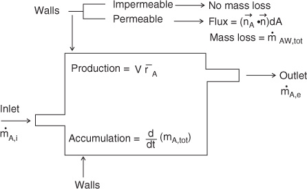
Diagrammatic illustration of macroscopic balance's control volume and control surface.

Figure 3.1 Simplified representation commonly used in macroscopic balances. Mass (shown in the figure) or mole units can be used.

The control volume is enclosed by a control surface as shown in Figure 3.1. The control surface is usually split into four parts for convenience of model formulation: an inlet, an outlet, a permeable wall region or an interface or catalytic surface, and an impermeable or inert wall or interface from which no transfer is taking place. Mass can cross into or out of the control volume from these surfaces, except from the impermeable or inert part of the surface. In addition, species mass is generated or consumed by chemical reaction. Finally, species mass can accumulate within the control volume as well for non-steady state conditions.

These components are then organized into the conservation law:

In from incoming flow – out from outgoing flow – transferred to the wall/interface + produced by reaction = accumulation

Molar units are more convenient for chemically reacting systems since the various species react or form according to their stoichiometric proportions. We use $M$ $M$ to denote moles here and $(\dot{M})$ $(\dot{M})$ to denote the molar flow rates. Hence the macroscopic balance is represented as

\begin{matrix} \begin{matrix} {\begin{matrix} \dot{\begin{matrix} M \end{matrix}} \end{matrix}}_{A, i} - {\begin{matrix} \dot{\begin{matrix} M \end{matrix}} \end{matrix}}_{A, e} - {\begin{matrix} \dot{\begin{matrix} M \end{matrix}} \end{matrix}}_{A, W} + V 〈 R_{A} 〉 = \frac{d}{d t} (\begin{matrix} {\begin{matrix} M \end{matrix}}_{A} \end{matrix}) \end{matrix} & (3.1) \end{matrix}

$\begin{matrix} \begin{matrix} {\begin{matrix} \dot{\begin{matrix} M \end{matrix}} \end{matrix}}_{A, i} - {\begin{matrix} \dot{\begin{matrix} M \end{matrix}} \end{matrix}}_{A, e} - {\begin{matrix} \dot{\begin{matrix} M \end{matrix}} \end{matrix}}_{A, W} + V 〈 R_{A} 〉 = \frac{d}{d t} (\begin{matrix} {\begin{matrix} M \end{matrix}}_{A} \end{matrix}) \end{matrix} & (3.1) \end{matrix}$

which is a general form applicable as a starting point in macroscopic modeling. Equation 3.1 applies for all the species present in the system—A, B, and so on. Equation 3.1 can also be formulated on a mass basis.

The control volume does not tend to zero, so local information is therefore lost. Each term in Equation 3.1, then, is an integral of local values. This point must be kept in mind in completing the model. Since local information is not available, some approximations must be introduced when formulating each of these terms. Let us now define each term as an integral of the local values to see how the terms can be closed by defining and using additional transport parameters.

3.1.1 In and Out Terms from Flow

In and out terms are normally calculated based on the flow rates at the inlet and outlet. Thus

\begin{matrix} in & = & {\dot{M}}_{A, i} = Q_{i} C_{A, i} \\ out & = & {\dot{M}}_{A, i} = Q_{e} C_{A, e} \end{matrix}

$\begin{matrix} in & = & {\dot{M}}_{A, i} = Q_{i} C_{A, i} \\ out & = & {\dot{M}}_{A, i} = Q_{e} C_{A, e} \end{matrix}$

where Q represents the volumetric flow rate. A similar expression is used at the outlet. In these expressions, i represents the inlet and e the exit.

Note: This representation assumes a uniform velocity in the inlet and outlet pipes. Otherwise, the concentration values, C_A,i and C_A,e, should be interpreted as the cup mixing (flow weighted) average values.

The volumetric flow rates at the inlet and exit can be calculated from the total molar flow rate $\dot{M}$ $\dot{M}$ and the total molar concentration, C. The relation is

Q = \dot{M} / C

$Q = \dot{M} / C$

where $\dot{M}$ $\dot{M}$ is the total molar flow rate (at inlet or outlet). The total molar concentration C is an intensive mixture property that can be calculated using some appropriate thermodynamic relation and depends on the mixture composition. Note that the volumetric flow rate at the inlet may be different from that at the exit, particularly for gas-phase systems with reactions that lead to appreciable mole change or for non-isothermal conditions. For liquid-phase systems, the volumetric flow rate at the inlet and outlet are usually assumed to be equal.

3.1.2 Wall or Interface Transfer Term

The local rate of mass transfer to the wall is related to the local flux vector. Thus, if n is a unit normal in the outward direction from the wall at a specified point, then the quantity transported is [N_A · n]dA. The integral of this over the permeable wall area represents the quantity transported to the wall:

{\dot{M}}_{A, W} = \int_{A_{w}} (N_{A} \cdot n) d A

${\dot{M}}_{A, W} = \int_{A_{w}} (N_{A} \cdot n) d A$

This information is based on the differential modeling concept, which needs the local or pointwise value of the flux vector and is not available in the macroscopic model. It is necessary to model this flux by using a mass transfer coefficient. Usually an overall mass transfer coefficient designated as ${\bar{K}}_{m}$ ${\bar{K}}_{m}$ is used and the flux to the wall is modeled as

\begin{matrix} {\dot{M}}_{A, W} = {\bar{K}}_{m} A_{w} (H_{A} < C_{A} > - {< C_{A} >}_{e x t}) & (3.2) \end{matrix}

$\begin{matrix} {\dot{M}}_{A, W} = {\bar{K}}_{m} A_{w} (H_{A} < C_{A} > - {< C_{A} >}_{e x t}) & (3.2) \end{matrix}$

The driving force for mass transfer is based on some average concentration difference. Here < C_A > is the average concentration in the control volume. It is corrected for the thermodynamic jump by multiplying by the Henry’s law parameter H_A. Note that we define H_AC_A(phase 1) = C_A(phase 2) as the thermodynamic relation for A between the two phases. The quantity < C_A >_ext is some average concentration in the external phase. Thus H_A < C_A > – < C_A >_ext is taken as an effective driving force for mass transfer.

An estimate of the average concentration in the control volume and in the external fluid is also needed, which will require some assumptions about the mixing pattern in the control volume or the tank as well as in the external fluid. In addition, the mass transfer coefficient ${\bar{K}}_{m}$ ${\bar{K}}_{m}$ is an average of the local values over the wall area. Local values may vary from point to point but an average value is used in the macroscopic model. ${\bar{K}}_{m}$ ${\bar{K}}_{m}$ is also an overall mass transfer coefficient from phase 1 to phase 2 (a combination of individual values)—a concept that is explained in detail in Chapter 6. Thus this model contains quite a few unknowns that we must close by making further approximations. These are better explained on a case-by-case basis. Thus, at this stage, we simply identify the closure problems associated with the mass transfer rate in the context of macroscopic models.

3.1.3 Rate Term

Mathematically, the average rate can be defined by the following equation:

< R_{A} > = \frac{1}{V} \int_{V} R_{A} (local) d V

$< R_{A} > = \frac{1}{V} \int_{V} R_{A} (local) d V$

where R_A is the local rate (in molar units) at any point in the system corresponding to the local concentration, and V is the volume of the system. In the macroscopic analysis, there is no way to calculate this rate, since the local concentration values are not being computed. The information loss principle dictates that some assumption on the level of mixing is needed to approximate the average rate term. One assumption is that the reactor is well mixed so that the concentration in the reactor is the same at every point. This so-called back-mixed model assumption is discussed in Section 3.6. Other assumptions are discussed in Section 3.7.

3.1.4 Accumulation Term

The term on the RHS of Equation 3.1 is the accumulation term—that is, the time rate of change of total moles of A in the system. The total moles of A is given as the integral of the local concentration of A at any point:

M_{A} = \int_{V} C_{A} d V = V 〈 C_{A} 〉

$M_{A} = \int_{V} C_{A} d V = V 〈 C_{A} 〉$

Again, some assumption about the mixing level is needed to assign the value for the average concentration.

Application of macro-models is now illustrated with several examples in which we indicate how the models could be closed by making suitable assumptions and using some additional model parameters.

3.2 The Batch Reactor

The first and perhaps simplest example of a macroscopic model is a batch reactor. In a typical batch reactor, the reactants are charged initially and a specified amount of time, called the batch time, is set to allow the reaction to proceed. Batch reactors are widely used in laboratory evaluation of processes, pilot-scale testing, and even commercial production of specialty or fine chemicals produced at a small scale (usually 500 Mt/year). For larger scales of production, continuous reactors are more economical.

3.2.1 Differential Equations for the Reactor

The mathematical model for a batch reactor is simple because the in and out terms are zero. The reactor is assumed to be well mixed so that there is no concentration variation locally with position in the entire control volume. Hence the macroscopic balance for the control volume (usually the liquid in the tank or reactor) reads as follows:

Accumulation = Net produced by reaction

In this setting, the mathematical statement given by Equation 3.1 simplifies to

\begin{matrix} \frac{d}{d t} (M_{A}) = {V R}_{A} & (3.3) \end{matrix}

$\begin{matrix} \frac{d}{d t} (M_{A}) = {V R}_{A} & (3.3) \end{matrix}$

where the <> notation for the rate term is suppressed because the reactor is assumed to be well mixed and is at a uniform concentration.

For a batch case, $M$ $M$ _A = C_AV and hence

\begin{matrix} \begin{matrix} \begin{matrix} \frac{d}{d t} \end{matrix} (C_{A} V) = {V R}_{A} \end{matrix} & (3.4) \end{matrix}

$\begin{matrix} \begin{matrix} \begin{matrix} \frac{d}{d t} \end{matrix} (C_{A} V) = {V R}_{A} \end{matrix} & (3.4) \end{matrix}$

Rate and Rate Function

The rate of production is a function of the concentrations and can be represented as

\begin{matrix} R_{A} = ν_{A} R (C_{A}, C_{B}, \dots, T) & (3.5) \end{matrix}

$\begin{matrix} R_{A} = ν_{A} R (C_{A}, C_{B}, \dots, T) & (3.5) \end{matrix}$

for a single reaction of the type

ν_AA + ν_BB + ... = 0

where ν_A, ν_B, . . . are the stoichiometric coefficients of A in the reaction. These coefficients are assigned positive values for products and negative values for reactants.

The parameter $R$ $R$ is called the rate function or the intrinsic kinetic model for the reaction or the species-independent rate of reaction. Note that the rate for any species, i, is simply given as

R_{i} = ν_{i} R

$R_{i} = ν_{i} R$

If the expression for the rate function is known, along with how the volume changes in the reactor as a function of time due to the change in the composition in the batch reactor, then Equation 3.4 can be integrated (usually numerically) to simulate the batch reactor.

For a first-order reaction, the rate function is represented as k₁C_A. The k₁ value is a first-order rate constant that is a function of temperature:

R (first order) = k_{1} C_{A} = A_{f} exp (- E / R_{g} T) C_{A}

$R (first order) = k_{1} C_{A} = A_{f} exp (- E / R_{g} T) C_{A}$

The Arrhenius law is used for the temperature dependency, where E is the activation energy and A_f is called the frequency factor. If the batch reactor is not isothermal, a heat balance equation for the temperature profile is needed in addition to the species mass balance equations. These equations are then solved simultaneously for C_A, C_B, . . ., and T .

Rate for Multiple Reactions

If there are two reactions, we can define a rate function for each reaction— say, $R$ $R$ ₁ and $R$ $R$ ₂. These are sufficient to define the rate of production of any species i:

R_{i} = ν_{1 i} R_{1} + ν_{2 i} R_{2}

$R_{i} = ν_{1 i} R_{1} + ν_{2 i} R_{2}$

or in general

R_{i} = Σ_{k}^{n r} ν_{k i} R_{k}

$R_{i} = Σ_{k}^{n r} ν_{k i} R_{k}$

where ν_ki is the stoichiometric coefficient of species i in the kth reaction. Here nr is the total number of independent reactions.

Constant Volume Analysis

For liquid systems, the density does not change significantly during the batch. Hence a constant volume is assumed and the model is simplified even further:

\begin{matrix} \frac{{d C}_{A}}{d t} = R_{A} with A, B, C, \dots & (3.6) \end{matrix}

$\begin{matrix} \frac{{d C}_{A}}{d t} = R_{A} with A, B, C, \dots & (3.6) \end{matrix}$

For simple linear cases, the equations can be integrated analytically. Consider a single species A participating in a reaction represented as follows:

A → B with R_A = –k₁C_A

The integrated form is

\frac{C_{A}}{C_{A i}} = exp (- k_{1} t)

$\frac{C_{A}}{C_{A i}} = exp (- k_{1} t)$

where C_Ai is the initial concentration of A in the reactor. The differential balance equation for B can be written and solved as well to obtain the product concentration as a function of time. However, an overall mass balance gives this concentration directly:

C_B = C_Bi + (C_Ai – C_A)

More generally, the batch reactor is solved using numerical methods. We now look at one such implementation in MATLAB.

3.2.2 ODE45 with CHEBFUN

The Runge-Kutta fourth- to fifth-order method is the workhorse for the numerical integration of a set of first-order differential equations. The MATLAB code ODE45 is an implementation of this method and is useful for this purpose. A sample driver is shown in Listing 3.1. The detailed mathematics underlying the Runge-Kutta method is not shown here, however; other books should be consulted for this explanation. The purpose here is to provide illustrative code that you can modify and use for many applications.

Listing 3.1 MATLAB Code for Solution of an Initial Value Problem

Click here to view code image

function odemain
global param1 param2 % parameters to be given to function dydt.
param1 = 2.0; param2=0.0;;
y0 = [1] % vector of initial values
tspan = linspace (0, 2, 11) ; % time intervals of solution
[ t y] = ode45 (@fun1, tspan, y0) % calling routine
plot (t,y) % solutions; A plot is generated

% function subroutine follows:
% This could be output into a separate file.
function dydt = fun1 (t, y)
global param1 param2
dydt = –param1*y; % simple first–order equation
% Add dydy(2), etc., for additional equations.

CHEBFUN Wrapping

This section may be omitted without loss of continuity.

An alternative implementation of ODE45 uses CHEBFUN, which provides a symbolic “feel” for the results with the efficiency of numerical computations. CHEBFUN helps to make the MATLAB codes easier and works with solutions as though they were analytic functions. The final results can be manipulated as though they were ordinary functions rather than numerical data. You will find it very useful once you start using these results.

CHEBFUN is a polynomial type of fitting of any given data or function using Chebecheff polynomials. Once fitted, these functions have the feel of a mathematical functions rather than a discrete set of data points. For more details, consult the papers by Battles and Trefethen (2004) and Trefethen (2007).

To get started, you need to type the following statement into the MATLAB command window:

Click here to view code image

unzip(’http://www.chebfun.org/download/chebfun_v4.2.2889.zip’)
cd chebfun_v4.2.2889, addpath(fullfile(cd,’chebfun’)), savepath

This code installs the CHEBFUN directory and adds the required path to the file. At this point, you will have access to a number of new functions that make the MATLAB coding easier. The code will look much more compact with this functionality added to your MATLAB program. Some sample codes provided in some exercise problems in this book use these compact functions.

The use of ODE45 with CHEBFUN is straightforward. The initial conditions are specified by the domain statement, which overloads the ODE45 function and creates a pseudo-analytical representation of the results rather than a set of tabular values. Listing 3.2 provides example code for a batch reactor in which the following reaction is taking place:

A → B → C

Here A forms B but B reacts further to form C. If C is an unwanted or waste product, we need to optimize the production of B. Too large a batch time is not desirable, while a too small value produces very little B, which is likewise not desirable. Hence the optimal batch time must be calculated. Additional details are provided in the following example.

Listing 3.2 MATLAB Code ODE45 with CHEBFUN Wrapping

Click here to view code image

% Consecutive reaction using ODE45 and CHEBFUN
% A → B → C; first–order reactions are used
% for illustration but the code can handle any nonlinear kinetics.
% Parameters used.
k1= 1.0; k2=2.0; tmax = 3.0;
C_init= [ 1 0 ] % vector of initial conditions
% Define functions to be solved.
fun = @(t,C) [–k1*C(1); k1*C(1) – k2*C(2)];
C = ode45(fun,domain(0,tmax), C_init); % solver
plot(C) % generates the plot

Example of a Series Reaction Simulation

In the code presented in this example, we simulate an isothermal system with a first-order reaction. Hence R_A = –k₁C_A and R_B = –k₂C_B + k₁C_A and the model equations to be solved are

\frac{{d C}_{A}}{d t} = - k_{1} C_{A}

$\frac{{d C}_{A}}{d t} = - k_{1} C_{A}$

and

\frac{{d C}_{B}}{d t} = - k_{2} C_{B} + k_{1} C_{A}

$\frac{{d C}_{B}}{d t} = - k_{2} C_{B} + k_{1} C_{A}$

with initial conditions of C_A = C_Ai and C_B = 0. Analytical solutions can obtained and compared with the numerical solution. In the code the concentrations are scaled by C_Ai; hence the initial conditions are taken as 1 and 0 for A and B, respectively.

An illustrative result is shown in Figure 3.2. It should be compared to the analytical solution to the model equations.

Graphical illustration of the result obtained with respect to the concentration profiles of species A and B in a batch reactor.

Figure 3.2 Concentration profiles for species A and B in a batch reactor simulated in MATLAB for a first-order reaction.

Additional postprocessing can be readily accomplished with CHEBFUN. For example, the concentration of B first increases with time and then decreases. The value of time at which the maximum concentration occurs is of importance, and here we show how to extract this value by postprocessing the concentration–time data. The lines of code shown in Listing 3.3 will do the postprocessing since CHEBFUB provides an analytic representation of the results.

Listing 3.3 Example of Postprocessing of CHEBFUN Results

Click here to view code image

c_max = max (C(:,2)) % finds what the maximum value is
F = diff(C(:,2)) % takes the derivative of variable two (species B)
roots(F) % finds where the maximum occurs

For the given example, the following analytical results can be calculated:

\begin{matrix} t_{o p t} = \frac{ln (k_{2} / k_{1})}{k_{2} - k_{1}} = 0.6931 & (3.7) \end{matrix}

$\begin{matrix} t_{o p t} = \frac{ln (k_{2} / k_{1})}{k_{2} - k_{1}} = 0.6931 & (3.7) \end{matrix}$

and

\begin{matrix} \frac{C_{B, max}}{C_{A i}} = {(k_{1} / k_{2})}^{[k_{2} / (k_{2} - k_{1})]} = 0.25 & (3.8) \end{matrix}

$\begin{matrix} \frac{C_{B, max}}{C_{A i}} = {(k_{1} / k_{2})}^{[k_{2} / (k_{2} - k_{1})]} = 0.25 & (3.8) \end{matrix}$

The simulations from the MATLAB-CHEBFUN program agree with the results of the analytical solution in an exact manner, thereby validating the code. Once the code has been validated, you can use it for more complex kinetics where the analytical solution is not generally available.

3.3 Reactor–Separator Combination

In this section, we consider a variation of the batch reactor, in which one of the products is volatile and is stripped to the gas phase by introduction of a purge gas. A schematic of this system is shown in Figure 3.3. Arrangements such as this are known as a reactor–separator combo (combination). In this example, we show that we can accomplish conversions larger than the equilibrium value because the product is stripped out of the reaction medium. This concept has many applications in reaction engineering. For example, a membrane reactor can be used to remove the product (e.g., hydrogen in steam reforming of methane), thereby improving the equilibrium conversion (see Section 27.4 for more details).

Diagrammatic representation of a batch reactor.

The diagram has two figures, the left representing the Equipment schematic and the right showing the Model representation. The equipment resembles a square block and has got Baffles on either side of the walls. The equipment is shown to have a Gas sparger at the bottom connected to a Gas In outlet at the top left, the vessel also has a Gas out outlet at top right. With this, the equipment is provided with a turbine stirrer. The Model representation of the equipment is as follows. A square block with two vertical partitions is shown. The left partition has a Gas in at the bottom and a Gas out at the top. The concentration of the content in this partition is "C subscript(B subscriptG)." The other partition is marked with a dashed vertical line in the middle of the box. This partition is shown to contain the Batch Liquid, with the contents' concentration marked as "C subscript A, C subscriptB, and C subscriptC." An arrow mark is drawn from the right partition to the left partition.

Figure 3.3 Schematic of a batch reactor with gas purging for simultaneous product removal.

Consider a reversible reaction represented by the following expression:

A ⇌ B + C

Let the rate be given by elementary kinetics:

R_A = –(k_f C_A – k_bC_BC_C)

where k_f is the rate constant for the forward reaction and k_b is the rate constant for the backward reaction. The two are related by the law of mass action, and k_f /k_b is equal to K_eq, the equilibrium constant for the reaction.

We assume A and C are nonvolatile and stay in the liquid phase. The differential equations for these processes are therefore

\frac{{d C}_{A}}{d t} = - (k_{f} C_{A} - k_{b} C_{B} C_{C})

$\frac{{d C}_{A}}{d t} = - (k_{f} C_{A} - k_{b} C_{B} C_{C})$

and

\frac{{d C}_{C}}{d t} = - (k_{f} C_{A} - k_{b} C_{B} C_{C})

$\frac{{d C}_{C}}{d t} = - (k_{f} C_{A} - k_{b} C_{B} C_{C})$

Now assume that B is a volatile product and is removed from the liquid by introducing some gas phase in the system. In this scenario, the mass balance for B should include a term to account for the transfer to gas phase. Species balance can be expressed in words as

Accumulation = In – out + generation – transferred to gas phase

with the in and out terms being zero for a batch reactor.

Putting this relationship in mathematical terms we have

\begin{matrix} \frac{d}{d t} ({V C}_{B}) = + V (k_{f} C_{A} - k_{b} C_{B} C_{C}) - {\dot{M}}_{B, \lg} & (3.9) \end{matrix}

$\begin{matrix} \frac{d}{d t} ({V C}_{B}) = + V (k_{f} C_{A} - k_{b} C_{B} C_{C}) - {\dot{M}}_{B, \lg} & (3.9) \end{matrix}$

where the last term is the transfer rate of moles of B from the liquid phase to the gas phase. The volume of the system is assumed to remain nearly constant—a reasonable assumption for liquid-phase systems or for reactions carried out with a solvent. Hence

\begin{matrix} \frac{{d C}_{B}}{d t} = (k_{f} C_{A} - k_{b} C_{B} C_{C}) - \frac{1}{V} {\dot{M}}_{B, \lg} & (3.10) \end{matrix}

$\begin{matrix} \frac{{d C}_{B}}{d t} = (k_{f} C_{A} - k_{b} C_{B} C_{C}) - \frac{1}{V} {\dot{M}}_{B, \lg} & (3.10) \end{matrix}$

A model for the for mass transfer from the liquid phase to the gas phase is now needed to close the transfer term. The concept of mass transfer coefficient is used here:

\begin{matrix} {\dot{M}}_{B, \lg} = {\bar{K}}_{m} A_{\lg} (H_{B} C_{B} - {〈 C_{B} 〉}_{g}) & (3.11) \end{matrix}

$\begin{matrix} {\dot{M}}_{B, \lg} = {\bar{K}}_{m} A_{\lg} (H_{B} C_{B} - {〈 C_{B} 〉}_{g}) & (3.11) \end{matrix}$

where H_B is the Henry’s law constant for B.

{\bar{K}}_{m}

${\bar{K}}_{m}$ is an average overall mass transfer coefficient from the liquid phase to the gas phase, and A_lg is the total gas–liquid interfacial area for mass transfer. < C_B >_g is the average concentration in the gas-phase. Modeling this system will require a gas-phase mass balance and some assumption on the extent of mixing in the gas phase. The gas phase balance in words is

In – Out + transferred to gas phase from liquid = Accumulation in the gas phase

The in term is zero if an inert gas is being used as purge gas. A further assumption is to neglect the accumulation term, decision called a pseudo-steady state approximation. It is usually justified since the gas volume in the system is smaller than the liquid volume.

The simplest model is to assume that the gas phase is mixed and that the representative concentration in the gas phase is the same as the exit gas concentration. Hence the moles out is $Q_{G, e} {< C_{B} >}_{g}$ $Q_{G, e} {< C_{B} >}_{g}$ . The gas-phase balance with this assumption of backmixing is

\begin{matrix} - Q_{G, e} {< C_{B} >}_{g} + {\bar{K}}_{m} A_{\lg} (H_{B} C_{B} - {< C_{B} >}_{g}) = 0 & (3.12) \end{matrix}

$\begin{matrix} - Q_{G, e} {< C_{B} >}_{g} + {\bar{K}}_{m} A_{\lg} (H_{B} C_{B} - {< C_{B} >}_{g}) = 0 & (3.12) \end{matrix}$

where a pseudo-steady state assumption is also used. This means that the gas phase concentration changes slowly over time and the accumulation term in the gas phase is neglected. The < C_B >_g represents the value of the average concentration of B in the gas phase. The average value is also the exit concentration, if the gas is assumed to well mixed.

Rearranging Equation 3.12 leads to the following expression:

\begin{matrix} {< C_{B} >}_{g} = \frac{{\bar{K}}_{m} A_{\lg} H_{B}}{{\bar{K}}_{m} A_{\lg} + Q_{G, e}} \cdot C_{B} & (3.13) \end{matrix}

$\begin{matrix} {< C_{B} >}_{g} = \frac{{\bar{K}}_{m} A_{\lg} H_{B}}{{\bar{K}}_{m} A_{\lg} + Q_{G, e}} \cdot C_{B} & (3.13) \end{matrix}$

When this definition is used in Equation 3.11, the mass transfer rate is modeled (after minor algebra) as

\begin{matrix} {\dot{M}}_{B, \lg} = Q_{G, e} H_{B} C_{B} [\frac{{\bar{K}}_{m} A_{\lg}}{{\bar{K}}_{m} A_{\lg} + Q_{G, e}}] & (3.14) \end{matrix}

$\begin{matrix} {\dot{M}}_{B, \lg} = Q_{G, e} H_{B} C_{B} [\frac{{\bar{K}}_{m} A_{\lg}}{{\bar{K}}_{m} A_{\lg} + Q_{G, e}}] & (3.14) \end{matrix}$

The differential equation for the concentration of B (Equation 3.8) can be completed by substitution of this term. The three equations (for A, B, and C) can then be solved simultaneously by using the numerical solver to simulate the concentration profiles as a function of time.

Note that Equation 3.14 reduces to $Q_{G, e} H_{B} C_{B}$ $Q_{G, e} H_{B} C_{B}$ when the mass transfer coefficient is relatively large. You may want to think about a physical interpretation of this observation.

Another point to note is that < C_B >_g is a function of time, although Equation 3.13 does reflect this relationship. C_B is a function of time as per Equation 3.10 and hence < C_B >_g is indirectly a function of time.

Example 3.1 Batch Reactor with Product Removal

Consider a constant volume batch reactor with a volume of reactor of 0.0982 m³, charged with 2000 mol/m³ of A, which reacts to form B and C. The reaction is reversible with the rate constants k_f = 1 hr^–1 and k_b = 5 × 10^–4 m³/mol s at the operating temperature. Simulate this with ODE45. What is the final product composition?

Now consider that B is being removed by purging with an inert gas. The gas flow rate is Q_G = 35 m³/hour.

The Henry’s law coefficient for product B is H_B = 2.2 × 10⁴ expressed as a concentration ratio.

Also assume that the overall mass transfer coefficient as infinity. This provides an upper bound and gives an equilibrium model, in which the exit gas is assumed to be in equilibrium with the liquid.

Simulate the reactor for the conditions stated and show that all A can be converted under these conditions.

Solution

Let ζ moles of A be reacted at final condition. Then C_A = 2000 – ζ, C_B = ζ, and C_C = ζ.

The law of mass action applies at equilibrium:

\frac{C_{C} C_{B}}{C_{A}} = \frac{ζ ζ}{2000 - ζ} = K_{e q} = \frac{k_{f}}{k_{b}} = 1 / 5 \times 10^{- 4} = 2000 {mol/m}^{3}

$\frac{C_{C} C_{B}}{C_{A}} = \frac{ζ ζ}{2000 - ζ} = K_{e q} = \frac{k_{f}}{k_{b}} = 1 / 5 \times 10^{- 4} = 2000 {mol/m}^{3}$

Solving this expression as a quadratic equation, ζ = 1236 mol/m³. The final composition should be then C_A = 764, C_B = 1236, and C_C = 1236, all in mol/m³.

The result of the MATLAB simulation is shown as a dotted line in Figure 3.4. The concentration of B attains a plateau, which is the equilibrium value of 1236 mol/m³.

Figure 3.4 Concentration profile for product B in the batch liquid with (solid line) and without product (dotted line) removal.

Now consider the effect of a gas purge that strips B from the liquid. The differential equation for species B is now modified by subtracting the ${\dot{M}}_{B, \lg}$ ${\dot{M}}_{B, \lg}$ term. The results are shown in Figure 3.4. The concentration of B does not reach an asymptotic equilibrium value, but rather keeps decreasing with time as it is being transferred to the gas phase. Correspondingly, the conversion of A exceeds the equilibrium value.

The key points to notice when modeling this problem are that a macroscopic balance for the gas phase is used in conjunction with a macroscopic balance for the batch liquid. In addition, some average concentration in the gas phase needs to be assigned and this assignment will depend on the mixing pattern of the gas phase. The exit concentration was assigned in the example, which is appropriate if the gas phase is assumed to be backmixed. If the gas were in plug flow, however, the logarithmic average of the inlet and the outlet concentration would be used, as discussed in the context of the mesoscopic model in Chapter 4.

3.4 Sublimation of a Spherical Particle

Let us now consider a different problem, in which we once again demonstrate the use of the mass transfer coefficient. The problem deals with a spherical particle that has appreciable vapor pressure and sublimes into the gas phase. The initial radius is R_i and the change in radius due to sublimation is to be calculated as a function of time. Figure 3.5 provides a schematic description of this problem. The sphere at the current instant of time is taken as the control volume. Let us use Equation 3.1 to set up the basic model, keeping only the relevant terms. In this scenario, there is no in term. Mass is lost from the surface by evaporation, which serves as the out term. Hence

Diagrammatic representation of a sublimation of a spherical particle.

Figure 3.5 Schematic of a sublimation of a solid.

–Out (from surface) = Accumulation

The out term is represented as ${\dot{M}}_{A}$ ${\dot{M}}_{A}$ , the evaporation rate.

Accumulation is the time rate of change of moles in the control volume. Moles equals mass divided by the molecular weight of the solid and is equal to (4/3)πR³ ρ_s/M_A, where R is the particle radius at the current value of time, ρ_s is the mass density of the solid, and M_A is the solid’s molecular weight. In turn, accumulation is the time derivative of this term. This accumulation term (which will have a numerically negative value) is balanced by the loss from the solid:

\begin{matrix} \frac{d}{d t} (\frac{4}{3} π R^{3} \cdot \frac{ρ_{s}}{M_{A}}) = - {\dot{M}}_{A} & (3.15) \end{matrix}

$\begin{matrix} \frac{d}{d t} (\frac{4}{3} π R^{3} \cdot \frac{ρ_{s}}{M_{A}}) = - {\dot{M}}_{A} & (3.15) \end{matrix}$

This provides the basic model based on the conservation principle.

The rate of evaporation appears as a term and has to be closed by using some transport law. Here, we define and use the following mass transfer coefficient:

Mass transfer rate from a surface per unit surface area = Mass transfer coefficient times a driving force

Let k_m be defined as the mass transfer coefficient with units of m/s. The driving force is taken as the concentration (in the gas) near the solid C_As minus the concentration in the gas far away from the solid surface, in the bulk gas C_A∞:

{\dot{M}}_{A} = 4 π R^{2} k_{m} (C_{A s} - C_{A \infty})

${\dot{M}}_{A} = 4 π R^{2} k_{m} (C_{A s} - C_{A \infty})$

The value of C_As is the concentration on the gas side of the interface. It can be calculated from the vapor pressure data of the subliming solid. The value of C_A∞ is usually taken as zero because the concentration of A gets very diluted in the regions away from the solid.

Using the expression for the transfer rate in Equation 3.15 and doing some minor simplification leads to

\begin{matrix} \frac{ρ_{s}}{M_{A}} (\frac{d R}{d t}) = - k_{m} (C_{A s} - C_{A \infty}) & (3.16) \end{matrix}

$\begin{matrix} \frac{ρ_{s}}{M_{A}} (\frac{d R}{d t}) = - k_{m} (C_{A s} - C_{A \infty}) & (3.16) \end{matrix}$

This equation can be integrated if the dependency of the mass transfer coefficient on the radius is known. In general, k_m is not a constant, but rather a function of the particle radius R. Commonly empirical correlations are used to connect these quantities. Let us review a commonly used correlation.

3.4.1 Correlation for Mass Transfer Coefficient

In general, the mass transfer coefficient is expected to be a function of the parameters indicated in the following equation:

k_m = f(d_p, D_A, v_∞, ρ_g, μ_g)

Data are usually correlated in terms of dimensionless parameters:

Sherwood number, S h = \frac{k_{m} d_{p}}{D_{A}}

$Sherwood number, S h = \frac{k_{m} d_{p}}{D_{A}}$

Reynolds number, Re = \frac{d_{p} ρ_{g} υ_{\infty}}{μ_{g}}

$Reynolds number, Re = \frac{d_{p} ρ_{g} υ_{\infty}}{μ_{g}}$

Schmidt number, S c = \frac{μ_{g}}{ρ_{g} D_{A}} = \frac{ν_{g}}{D_{A}}

$Schmidt number, S c = \frac{μ_{g}}{ρ_{g} D_{A}} = \frac{ν_{g}}{D_{A}}$

A commonly used correlation is that developed by Froessling (1938) and Ranz and Marshall (1952):

\begin{matrix} S h = 2 + 0.552 {Re}^{1 / 2} {S c}^{1 / 3} & (3.17) \end{matrix}

$\begin{matrix} S h = 2 + 0.552 {Re}^{1 / 2} {S c}^{1 / 3} & (3.17) \end{matrix}$

This correlation is valid for Re from 2 to 800 and for Sc from 0.6 to 2.7 (typical range for gases), and can be used to find k_m as a function of particle diameter or radius. For a stagnant gas, Re = 0 and therefore Sh = 2. Hence the mass transfer coefficient is given as

\begin{matrix} k_{m} (sphere to a stagnant gas) = \frac{2 D_{A}}{d_{p}} = \frac{D_{A}}{R} & (3.18) \end{matrix}

$\begin{matrix} k_{m} (sphere to a stagnant gas) = \frac{2 D_{A}}{d_{p}} = \frac{D_{A}}{R} & (3.18) \end{matrix}$

Note that k_m is an inverse function of the particle radius. Equation 3.18 is a theoretical result and is derived in Example 6.2.

For a flowing gas, the second term in Equation 3.17 is more important. At high velocity, we can deduce from this equation that $k_{m} \propto d_{p}^{- 1 / 2}$ $k_{m} \propto d_{p}^{- 1 / 2}$ at high flow rates. In general, therefore, we can expect k_m to vary as $d_{p}^{- a}$ $d_{p}^{- a}$ , where a is an exponent in the range of 1/2 to 1. The dependency of the mass transfer coefficient on the radius must be included when integrating Equation 3.16. The following example shows the integrated result for a no-flow condition.

Example 3.2 Rate of Shrinkage of a Subliming Sphere

A naphthalene ball (M_A = 128 g/mol and ρ_s = 1145 kg/m³) is suspended in still air at 347 K and 1 atm pressure. Estimate the time to reduce the diameter from 2 cm to 0.5 cm for the following parameter values: D_A = 8.19 × 10^–6 m²/s and the vapor pressure of naphthalene is 666 Pa for the given temperature.

Solution

Equation 3.18 applies to a scenario involving still air, and we can replace the mass transfer coefficient by D_A/R in Equation 3.14. Also, far from the solid, the naphthalene concentration, C_A∞, can be assumed to zero. Hence

\begin{matrix} \frac{ρ_{s}}{M_{A}} (\frac{d R}{d t}) = - \frac{D_{A}}{R} C_{A s} & (3.19) \end{matrix}

$\begin{matrix} \frac{ρ_{s}}{M_{A}} (\frac{d R}{d t}) = - \frac{D_{A}}{R} C_{A s} & (3.19) \end{matrix}$

The variables can be separated:

\int_{R_{i}}^{R_{f}} R d R = \frac{D_{A} M_{A}}{ρ_{s}} C_{A s} \int_{0}^{t} d t

$\int_{R_{i}}^{R_{f}} R d R = \frac{D_{A} M_{A}}{ρ_{s}} C_{A s} \int_{0}^{t} d t$

This is followed by integration:

R_{i}^{2} - R_{f}^{2} = [\frac{D_{A} M_{A}}{ρ_{s}} C_{A s}] \cdot t

$R_{i}^{2} - R_{f}^{2} = [\frac{D_{A} M_{A}}{ρ_{s}} C_{A s}] \cdot t$

For numerical calculations, it is easier to regroup the bracketed term on the LHS as K and write this expression as

R_{f}^{2} = R_{i}^{2} - K t

$R_{f}^{2} = R_{i}^{2} - K t$

The radius is seen to decrease as the square root of time.

Mathematical description of problems in which the size of a solid decreases due to chemical reaction with a gas has a similar structure and is discussed in Section 19.2. The dependency of the radius on time has a similar form with a square root dependency.

3.5 Dissolved Oxygen Concentration in a Stirred Tank

Now consider another application of the concept of mass transfer coefficient. The problem statement is as follows: Oxygen gas is continuously bubbled into a pool of liquid of volume V_L and the liquid becomes saturated with oxygen with the passage of time. The dissolved oxygen concentration can be measured with an oxygen probe as a function of time. We will develop a model to predict this transient oxygen concentration profile. The time needed for, say, 90% saturation can be calculated by this model. The problem can be approached by a macroscopic balance where we take the total liquid volume as the control volume and write the conservation law.

The input term in this case is the oxygen crossing into the liquid from the gas–liquid interface. Let us denote this term as ${\dot{M}}_{A}$ ${\dot{M}}_{A}$ (mol/s).

There is no output term since there is no liquid leaving the system.

There is no chemical reaction, so the generation term is zero.

Finally, the accumulation term is the time derivative of dissolved oxygen in the tank. It is equal to d/dt of (V_LC_A), where C_A is the oxygen concentration in the tank. We assume that the concentration is uniform everywhere in the liquid because the tank is well agitated. Hence there is no need to distinguish between < C_A > and C_A.

For this scenario, the macroscopic conservation statement is

{\dot{M}}_{A} = \frac{d}{d t} (V_{L} C_{A})

${\dot{M}}_{A} = \frac{d}{d t} (V_{L} C_{A})$

The liquid volume in the tank is assumed to remain constant and V_L can be pulled out, leaving us with

\begin{matrix} V_{L} \frac{{d C}_{A}}{d t} = {\dot{M}}_{A} & (3.20) \end{matrix}

$\begin{matrix} V_{L} \frac{{d C}_{A}}{d t} = {\dot{M}}_{A} & (3.20) \end{matrix}$

A model (a transport law) is needed to close ${\dot{M}}_{A}$ ${\dot{M}}_{A}$ , the rate of gas–liquid mass transfer. Again, this is closed in the context of macroscopic models using a mass transfer coefficient. The driving force is the oxygen saturation solubility, $C_{A}^{*}$ $C_{A}^{*}$ , minus the instantaneous oxygen concentration in the liquid, C_A. Hence the molar rate of transfer of oxygen is modeled as

\begin{matrix} {\dot{M}}_{A} = k_{L} a_{g l} (C_{A}^{*} - C_{A}) V_{R} & (3.21) \end{matrix}

$\begin{matrix} {\dot{M}}_{A} = k_{L} a_{g l} (C_{A}^{*} - C_{A}) V_{R} & (3.21) \end{matrix}$

where k_L is the local mass transfer coefficient from a bubble surface to a bulk liquid, defined per unit area of the interface. We multiply this coefficient first by a_gl, the interfacial area per unit volume of the dispersion (gas + liquid), and then we multiply it by V_R, the total dispersion volume, to get ${\dot{M}}_{A}$ ${\dot{M}}_{A}$ as shown in the previous equation.

The parameter k_La_gl is called the overall or volumetric mass transfer coefficient since it gives the transfer rate per unit volume; in contrast, the parameter k_L is called the intrinsic (liquid side) mass transfer coefficient. The latter is based on the unit area for mass transfer.

Using the expression for ${\dot{M}}_{A}$ ${\dot{M}}_{A}$ from Equation 3.21 in Equation 3.20, we get

\begin{matrix} V_{L} \frac{{d C}_{A}}{d t} = k_{L} a_{g l} V_{R} (C_{A}^{*} - C_{A}) & (3.22) \end{matrix}

$\begin{matrix} V_{L} \frac{{d C}_{A}}{d t} = k_{L} a_{g l} V_{R} (C_{A}^{*} - C_{A}) & (3.22) \end{matrix}$

The ratio V_L/V_R is generally denoted as liquid holdup ∊_l. Hence we have

\begin{matrix} \frac{{d C}_{A}}{d t} = \frac{k_{L} a_{g l}}{ε_{L}} (C_{A}^{*} - C_{A}) & (3.23) \end{matrix}

$\begin{matrix} \frac{{d C}_{A}}{d t} = \frac{k_{L} a_{g l}}{ε_{L}} (C_{A}^{*} - C_{A}) & (3.23) \end{matrix}$

The initial condition C_A = 0 at time t = 0 is used. The integrated solution is

\begin{matrix} \frac{C_{A}}{C_{A}^{*}} = 1 - exp (- \frac{k_{L} a_{g l}}{ε_{L}} t) & (3.24) \end{matrix}

$\begin{matrix} \frac{C_{A}}{C_{A}^{*}} = 1 - exp (- \frac{k_{L} a_{g l}}{ε_{L}} t) & (3.24) \end{matrix}$

The measurement of dissolved oxygen concentration thus provides a useful experimental tool to measure the overall mass transfer coefficient, k_La_gl, in the equipment.

A question for discussion is how the model changes if air is bubbled into the liquid, rather than pure oxygen being the gas applied. The value of $C_{A}^{*}$ $C_{A}^{*}$ will now depend on the representative oxygen partial pressure in the gas phase. This will, in turn, need a model for the gas phase and some assumption about the mixing pattern in the gas.

3.6 Continuous Stirred Tank Reactor

Section 3.2 considered the simulation of a batch reactor. In this section we model a continuous stirred tank reactor (CSTR). In this system, a reactant stream enters continuously in a tank that is well stirred. A chemical reaction takes place in the tank, and the product stream is withdrawn in a continuous manner. The schematic for this system is shown in Figure 3.6. We construct a macroscopic model and close it by using the backmixing assumption. The well-mixed model assumption is that the concentration in the tank is uniform and equal to the exit concentration; it is used to close the rate term as discussed further in this section.

Diagrammatic representation of a well-mixed reactor.

Figure 3.6 Schematic representation of a well-mixed reactor, the continuous stirred tank reactor (CSTR).

The conservation law is:

in – out + generation = 0

The various terms can be calculated as follows and put into an algebraic equation:

Moles of A in = QC_A,i

Moles of A out = QC_A,e

Hence

\begin{matrix} {Q C}_{A, i} - {Q C}_{A, e} + V < R_{A} > = 0 & (3.25) \end{matrix}

$\begin{matrix} {Q C}_{A, i} - {Q C}_{A, e} + V < R_{A} > = 0 & (3.25) \end{matrix}$

We need to close < R_A > by making some assumptions about the level of mixing in the system. In this example, we assume complete backmixing. This assumption implies that the tank is well mixed, and that the concentration is the same everywhere and is equal to the exit concentration.

\begin{matrix} Backmixed tank model: C_{A} (tank) = C_{A, e} & (3.26) \end{matrix}

$\begin{matrix} Backmixed tank model: C_{A} (tank) = C_{A, e} & (3.26) \end{matrix}$

This simplification arises because the contents of a well-mixed tank have the same composition, which is also the same as the exit concentration. Model results for first-order and second-order reactions are presented next.

3.6.1 First-Order Reaction

The generation rate due to reaction is calculated as –V kC_A(tank) = –V kC_A,e. Here k is the rate constant of the first-order reaction.

The generation rate is assigned a negative sign because A is consumed by reaction. Also, the backmixed assumption permits us to write the rate in terms of the exit concentration, which we want to calculate.

Putting all the terms together, we have the following equation for the change in concentration between the inlet and outlet streams in the tank:

\begin{matrix} {Q C}_{A, i} - {Q C}_{A, e} - {V k C}_{A, e} = 0 & (3.27) \end{matrix}

$\begin{matrix} {Q C}_{A, i} - {Q C}_{A, e} - {V k C}_{A, e} = 0 & (3.27) \end{matrix}$

This is the model for a backmixed reactor for a first-order reaction; it is widely used in chemical reaction engineering.

It is also convenient to work with dimensionless quantities. Let c_A = C_A/C_A,i, a measure of concentration. Let Da = V k/Q, a dimensionless rate constant; this is usually referred to as the Damkohler number in reaction engineering parlance. The Damkohler number is the ratio of the holding time, V/Q, or the residence time to the reaction time, 1/k.

The final solution to Equation 3.27 can be written compactly as follows:

\begin{matrix} c_{A, e} = \frac{C_{A, e}}{C_{A, i}} = \frac{1}{1 + D a} & (3.28) \end{matrix}

$\begin{matrix} c_{A, e} = \frac{C_{A, e}}{C_{A, i}} = \frac{1}{1 + D a} & (3.28) \end{matrix}$

We now mention a complication as a consequence of averaging and due to the different levels of mixing prevalent in flow systems, especially under turbulent flow conditions.

3.6.2 Second-Order Reaction

In this subsection, we look at a second-order reaction to see the additional closures that may be needed. The model equation is similar to Equation 3.25:

\begin{matrix} {Q C}_{A, i} - {Q C}_{A, e} + V < R_{A} > = 0 & (3.29) \end{matrix}

$\begin{matrix} {Q C}_{A, i} - {Q C}_{A, e} + V < R_{A} > = 0 & (3.29) \end{matrix}$

The average rate $< R_{A} > is - k_{2} < C_{A, e}^{2} >$ $< R_{A} > is - k_{2} < C_{A, e}^{2} >$ , the integral of the square of the exit concentration. Although the concentration in the reactor is assumed to be the same as the exit concentration, locally there may be a variance in the concentration. Hence $< C_{A, e}^{2} >$ $< C_{A, e}^{2} >$ , the integral of the square, need not be the same as (< C_A,e >)², the square of the integral. The two are equal if the concentration at each and every point is the same as C_A,e and, in addition, if there are no local fluctuations in the concentration. The backmixing assumption guarantees that the concentration, on average, at every point in the reactor is the same and also equal to the exit concentration. Nevertheless, that does not imply that there is no deviation from the average at every point. If there is no deviation (variance is zero) as well, the assumption is called a micromixed reactor. Hence the following additional assumption is made:

〈 C_{A, e}^{2} 〉 = C_{A e}^{2}

$〈 C_{A, e}^{2} 〉 = C_{A e}^{2}$

Once this assumption is made the rate term can be closed, leading to the following model for a second-order reaction:

\begin{matrix} {Q C}_{A, i} - {Q C}_{A, e} - V k_{2} C_{A, e}^{2} = 0 & (3.30) \end{matrix}

$\begin{matrix} {Q C}_{A, i} - {Q C}_{A, e} - V k_{2} C_{A, e}^{2} = 0 & (3.30) \end{matrix}$

This can be solved as a quadratic equation for the exit concentration. It is often solved using a dimensionless parameter, the Damkohler number, which is defined as follows for a second-order reaction:

D a = \frac{V k_{2} C_{A, i}}{Q}

$D a = \frac{V k_{2} C_{A, i}}{Q}$

The final result for the dimensionless exit concentration is

c_{A, e} = \frac{C_{A, e}}{C_{A, i}} = \frac{\sqrt{1 + 4 D a} - 1}{2 D a}

$c_{A, e} = \frac{C_{A, e}}{C_{A, i}} = \frac{\sqrt{1 + 4 D a} - 1}{2 D a}$

Similar models can be written for any other form of the rate equation and solved either by applying analytical methods or by using numerical algebraic solver routines.

The following discussion may be omitted on first reading.

A reactor analyzed as described in the preceding discussion is called a micromixed reactor with complete backmixing. In some cases, however, differences in the local concentration may exist, since the fluid elements entering at different times may not mix at a microscale and remain segregated. Models to account for this possibility can be developed at various levels of details. One such a model is called the segregated model or macrofluid model and is discussed here briefly.

Consider a point in the reactor and the time variation of the concentration as shown in Figure 3.7. The flow is usually turbulent and the concentrations fluctuate with time. If the fluctuations are small, their contributions to the rate can be neglected. The rate for a second-order reaction is then proportional to (C_Ae)², as in the completely micromixed model. Fluid elements must be mixed on a microscale for this assumption to hold.

Diagram shows two figures comparing the time variation of the concentration.

Figure 3.7 A qualitative illustration of macromixed and micromixed systems showing the presumed concentration variation at any point in the reactor as a function of time.

If the reactor contents are not completely micromixed, the fluctuating part of the concentration contributes to an extra rate in a time-averaged sense. Models incorporating the variance of the concentration distribution are needed to capture this effect (a topic briefly addressed in Chapter 13). A second limiting case, in which the fluid is assumed to be mixed only on a large scale, is known as macromixed or segregated model. In this model, the fluid elements are assumed to retain their identity from the time they enter the reactor to the time they exist from the reactor and to persist as separate segregated packets. These two limiting cases (micromixed and segregated) are used to bracket the performance for a non-first-order reaction.

The solution for the segregated model requires the concept of exit age distribution and is postponed to a later chapter in Section 13.5. To help you get a feel for the numbers, Table 3.1 gives the solution for the two models.

Table 3.1 Comparison of Micro Versus Segregation Model for a Backmixed Reactor for Second-Order Kinetics

Da	c_A,e, Microfluid	c_A,e, Macrofluid
0.1	0.9161	0.9156
1.0	0.6180	0.5963
10.0	0.2702	0.2015
100.0	0.0951	0.0408

The following differences between the two limiting approaches to model a well-mixed reaction are important to note:

Whether the fluid is micromixed or macromixed makes no difference for a first-order reaction. Details are provided in Section 13.5.
The actual reactor performance is somewhere in between the two limiting cases for reactions involving nonlinear kinetics. To model this performance in more detail, a segregation parameter must be introduced.
The two models do not differ much at small values of Da, and the differences are significant only for fast reactions (larger values of Da).
The segregated flow model gives a higher conversion rate (1 – c_A,e) for a second-order reaction, as shown in Table 3.1.
The micromixed model gives a higher conversion rate for reaction orders less than 1 (results are not shown here but are discussed in Section 13.3).

3.7 Tracer Experiments: Test for Backmixed Assumption

The assumption of backmixing can be tested by performing tracer studies. In this kind of study, the feed solution is perturbed by adding a tracer and the exit concentration of the tracer is measured. A simple experiment, for instance, would be to replace water flowing in the tank with a NaCl solution. The concentration of NaCl in the exit flow is then measured. This type of experiment, which is called a step tracer experiment, is shown schematically in Figure 3.8.

Diagrammatic illustration of a step tracer experiment.

Figure 3.8 Illustrative representation of a step tracer experiment.

The response will be an exponential function of time if the system is well mixed. The following equation (derived in Section 13.2) is applicable to the transient response:

\begin{matrix} \frac{C_{A, e} (t)}{C_{A, i}} = 1 - exp (- t \frac{Q}{V}) & (3.31) \end{matrix}

$\begin{matrix} \frac{C_{A, e} (t)}{C_{A, i}} = 1 - exp (- t \frac{Q}{V}) & (3.31) \end{matrix}$

Any deviation of experimental data from this scenario indicates that the assumption of complete mixing may not be valid under the given conditions of flow rate. Other modes of injecting a tracer (e.g., pulse tracer) can also be used and the corresponding response examined. These details are taken up in Chapter 13.

3.7.1 Interconnected Cells Model

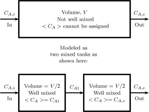
If a system is not backmixed, a model can be used in which the system is composed of a number of smaller macroscopic control volumes connected in series or parallel. Two examples of such models are described in this section. Modeling of each subunit is then done and the overall performance can be examined. More details are presented in Chapter 13.

In the first example, the reactor is modeled as two or more stirred tanks in series, shown schematically in Figure 3.9. The tracer data can be used to fit the equivalent number of well-mixed tanks needed to model the reactor. More details are presented in Section 13.3.

Diagrammatic illustration of a reactor modelled as two well mixed tanks connected in series.

The reactor is first shown as a single rectangular block to have an Inlet on the left with concentration C subscript(A, i) and an outlet on the right with concentration C subscript(A, e). The volume of the tank is V. The text inside the tank reads Not well mixed, C subscriptA cannot be assigned. This reactor is modeled as two mixed tanks as shown in the next sketch. The two well mixed tanks resemble two square blocks connected to each other with an arrow that flows from the first block to the next. The first block is shown to have an inlet on the left with concentration C subscript(A, i), and an outlet on the right with concentration C subscript(A1) which is the inlet to the next block, whose outlet concentration is C subscript(A, e). The volume of both tanks is "V by 2." The concentration of the first tank is C subscriptA equals C subscriptA1 and the concentration of the second tank is C subscriptA equals C subscript(A, e).

Figure 3.9 An equivalent two-tank representation of a reactor.

3.7.2 Model Composed of Active and Dead Zone

Another type of model used to account for deviations from a well-mixed tank incorporates a dead volume. Often the tank is nearly well mixed but mixing is poor in some regions in the tank—so-called dead zones. A model for such a system can be constructed as an active region and a dead region, as shown in Figure 3.10. A theoretical tracer response can be fitted to experimental data to ascertain the relative volume of the active zone and the dead zone as well as the rate of mass exchange between the two regions. The reactor model is then constructed by using two macroscopic control volumes connected with mass exchange.

Diagrammatic representation of a single stirred reactor with dead zones modelled as a two tanks connected in parallel.

Figure 3.10 A stirred reactor with some dead zones modeled as two tanks connected in parallel. Flow occurs in and out of the active or mixed tank, and a slow mass exchange is assumed between the dead zone and the active zone.

3.8 Liquid–Liquid Extraction

In this section we model a two-phase system in which a liquid–liquid extraction takes place. The mixer-settler shown in Figure 1.4 is analyzed here. In this equipment, a feed mixture consisting of components A (the solute to be extracted) and C (a carrier) enters the contactor. The feed is contacted with a solvent S, and species A is transferred to the solvent phase. The two phases are intimately mixed and then separated. The solvent phase called the extract while the carrier phase is called the raffinate. The problem is to calculate the exit composition of the separated mixture.

This system is modeled by using two control volumes: one for the aqueous (feed) phase and one for the solvent phase, as shown in Figure 3.11. The phases share a common interface, and mass is exchanged across the interface. The macroscopic balances are used for each compartment. The model shown in this section is based on the assumption that C is not soluble in the S phase, and vice versa; that is, there is no mutual solubility of C and S.

Diagrammatic representation of a liquid-liquid extraction as a two macroscopic control volumes.

Figure 3.11 Schematic of a liquid–liquid extractor modeled as two macroscopic control volumes.

The solute conservation is then applied to the two control volumes (feed phase and extract phase), as shown in Figure 3.11. It is preferable to use the mole ratio rather than the mole fractions since the total flow rate is changing from the inlet to the outlet due to the solute transfer. The mole ratio is defined as

X = \frac{x}{1 - x} and Y = \frac{y}{1 - y}

$X = \frac{x}{1 - x} and Y = \frac{y}{1 - y}$

Here x is the mole fraction of A in the feed phase and y is the mole fraction in the solvent phase. The subscript A for mole fraction is suppressed in this case, so, for example, x = x_A in this section. Note that for a dilute mixture, the mole ratio is nearly the same as the mole fraction. X = x and Y = y.

The balance of species A in the feed is

in – out – transferred to solvent phase = 0

Expressing this in mathematical terms, we have

\begin{matrix} F_{c} X_{f} - F_{c} X_{e} - {\dot{M}}_{A} = 0 & (3.32) \end{matrix}

$\begin{matrix} F_{c} X_{f} - F_{c} X_{e} - {\dot{M}}_{A} = 0 & (3.32) \end{matrix}$

where F_C is the flow rate of the solute-free aqueous phase. We assume that the component C (the carrier) is not transferred to the solvent phase; hence its flow rate remains F_C invariant. (This is the reason for using the mole ratio instead of mole fractions.)

The balance of A in the solvent phase is formulated in a similar manner:

in – out + received from the feed phase = 0

This can be written as

\begin{matrix} {S Y}_{f} - {S Y}_{e} + {\dot{M}}_{A} = 0 & (3.33) \end{matrix}

$\begin{matrix} {S Y}_{f} - {S Y}_{e} + {\dot{M}}_{A} = 0 & (3.33) \end{matrix}$

which is the mass balance in mole ratio form. Here S is the solvent flow rate on a solute-free basis. Again, we assume no solvent goes to the feed phase; that is, S has no solubility in the aqueous phase.

3.8.1 Mass Transfer Rate

A mass transfer rate model is now needed to close the ${\dot{M}}_{A}$ ${\dot{M}}_{A}$ term. The mass transfer coefficient is defined in these systems using an effective mole fraction difference as the driving force, rather than the concentration difference. Let < x > and < y > be representative average mole fractions in the carrier phase and the solvent phase. The thermodynamic equilibrium relation is usually represented in terms of a partition coefficient m:

\begin{matrix} y * = m x & (3.34) \end{matrix}

$\begin{matrix} y * = m x & (3.34) \end{matrix}$

where y* is the mole fraction corresponding to x if equilibrium were attained. Thus m < x > – < y > is the effective driving force.

The mass transfer rate is then the following term using the mole fraction difference as the driving force:

{\dot{M}}_{A} = K_{y} a_{l l} V_{d} (m 〈 x 〉 - 〈 y 〉)

${\dot{M}}_{A} = K_{y} a_{l l} V_{d} (m 〈 x 〉 - 〈 y 〉)$

where K_y is the intrinsic mass transfer coefficient, a_ll is the liquid–liquid transfer area per unit volume of the dispersion, and V_d is the volume of the dispersion.

The previous equation can also be expressed in terms of the mole ratio:

{\dot{M}}_{A} = K_{y} a_{l l} V_{d} (m \frac{< X >}{1 + < X >} - \frac{< Y >}{1 + < Y >})

${\dot{M}}_{A} = K_{y} a_{l l} V_{d} (m \frac{< X >}{1 + < X >} - \frac{< Y >}{1 + < Y >})$

3.8.2 Backmixed–Backmixed Model

In the previously described model, 〈X〉 and 〈Y〉 are representative concentrations of A in the system in the two phases. A further assumption about the mixing levels in the system is needed to assign values to these concentrations. One such assumption is that both phases are completely mixed, which leads to the backmixed–backmixed model. The < X > and < Y > concentrations are then assigned as the exit values and the mass transfer model is closed:

\begin{matrix} {\dot{M}}_{A} = K_{y} a_{l l} V_{d} (m \frac{X_{e}}{1 + X_{e}} - \frac{Y_{e}}{1 + Y_{e}}) & (3.35) \end{matrix}

$\begin{matrix} {\dot{M}}_{A} = K_{y} a_{l l} V_{d} (m \frac{X_{e}}{1 + X_{e}} - \frac{Y_{e}}{1 + Y_{e}}) & (3.35) \end{matrix}$

Model formulation is now complete, and Equations 3.32 and 3.33 are solved simultaneously using Equation 3.35 for the mass transfer rate. The MATLAB program FSOLVE or similar algebraic equation solvers can be used to solve the equations. The exit concentrations can thus be predicted for a given condition provided the values of the mass transfer coefficients are known. The overall mass transfer coefficient K_ya_ll is sufficient, and the intrinsic coefficient K_y and the interfacial area a_ll need not be known separately.

3.8.3 Equilibrium Stage Model

A simpler model often used as a first approximation in practice is the ideal stage model, which assumes that the mass transfer rate is sufficiently large so that the exit streams reach an equilibrium value. Conservation laws together with thermodynamics of phase equilibrium are used in model building for such processes.

Adding Equations 3.32 and 3.33 results in elimination of the mass transfer rate term:

F_CX_f – F_CX_e + SY_f – SY_e = 0

This is the overall mass balance for A for the entire equipment.

If the solvent contains no dissolved A, we set Y_f equal to zero. Hence

\begin{matrix} F_{c} X_{f} - F_{C} X_{e} - S Y_{e} = 0 & (3.36) \end{matrix}

$\begin{matrix} F_{c} X_{f} - F_{C} X_{e} - S Y_{e} = 0 & (3.36) \end{matrix}$

Now we assume that the exit streams are in equilibrium, thereby creating an equilibrium stage model. The equilibrium relation, which is usually expressed as the ratio of mole fractions in the two phases, is given by Equation 3.34. It can be recast in mole ratio form and expressed as

Y_e = K_AX_e

where K_A is the partition coefficient for A using the mole ratio units. This is related to the partition coefficient based on mole fraction units as follows:

K_{A} = m \frac{1 - x}{1 - y}

$K_{A} = m \frac{1 - x}{1 - y}$

Inserting this result in Equation 3.36, we have

\begin{matrix} F_{C} X_{f} - F_{C} X_{e} - S K_{A} X_{e} = 0 & (3.37) \end{matrix}

$\begin{matrix} F_{C} X_{f} - F_{C} X_{e} - S K_{A} X_{e} = 0 & (3.37) \end{matrix}$

Solving for the solute mole ratio in the exit of the feed, we find

\begin{matrix} X_{e} = \frac{X_{f}}{(1 + {S K}_{A} / F C)} & (3.38) \end{matrix}

$\begin{matrix} X_{e} = \frac{X_{f}}{(1 + {S K}_{A} / F C)} & (3.38) \end{matrix}$

This model for liquid–liquid extraction assumes an ideal stage concept. Note that the conservation law and thermodynamics have been used, but no mass transfer effects are considered. The mass transfer is considered to be almost complete in the equilibrium stage model. Often separation processes are first modeled by making such an assumption to obtain a quick estimate of the performance of the system under ideal conditions. The dimensionless group SK_A/F_C is called the extraction factor, denoted as E. Equation 3.38 can then be written in terms of the extraction factor:

\frac{X_{e}}{X_{f}} = \frac{1}{1 + E}

$\frac{X_{e}}{X_{f}} = \frac{1}{1 + E}$

The fractional removal of A denoted as ø_A in a single state extraction device is then given as

ϕ_{A} = \frac{E}{1 + E}

$ϕ_{A} = \frac{E}{1 + E}$

3.8.4 Stage Efficiency

The ideal stage model can be corrected in an empirical manner by using the concept of stage efficiency, η:

\begin{matrix} η = \frac{X_{f} - X_{e}}{X_{f} - X_{e}^{*}} & (3.39) \end{matrix}

$\begin{matrix} η = \frac{X_{f} - X_{e}}{X_{f} - X_{e}^{*}} & (3.39) \end{matrix}$

where $X_{e}^{*}$ $X_{e}^{*}$ is the solute concentration reached if equilibrium were achieved. This concentration is given by Equation 3.38. The stage efficiency depends on the mass transfer coefficient between the two phases, the interfacial area for mass transport, and the flow pattern of the two phases. Models for stage efficiency can be developed by solving the models including the rate mass transfer and comparing the results with the equilibrium model. More often, however, empirically based values for the stage efficiency (gained from prior design experience) are used.

For dilute systems with a constant value of m, the mass transfer model can be solved algebraically if both phases are assumed to be backmixed. Based on the result, the following relation can be derived for the stage efficiency.

\begin{matrix} η = \frac{k (1 + E)}{1 + k (1 + E)} & (3.40) \end{matrix}

$\begin{matrix} η = \frac{k (1 + E)}{1 + k (1 + E)} & (3.40) \end{matrix}$

Here κ is a dimensionless mass transfer coefficient κ defined as follows:

\begin{matrix} k = K_{y} a_{l l} S / F & (3.41) \end{matrix}

$\begin{matrix} k = K_{y} a_{l l} S / F & (3.41) \end{matrix}$

In this expression, S is the solvent flow rate and F is the feed flow rate. Both are nearly constant for dilute solutions.

As κ tends to ∞ (i.e., with a large mass transfer rate), the stage efficiency tends to 1.

Summary

Batch reactors are a well-studied problem in chemical kinetics, and the differential equations for the transient concentration profiles can be derived by balancing the accumulation to the rate of production. Spatial variations in the concentrations are usually small, so diffusional considerations are not important.
Models for batch reactors involving multiple reactions are solved by numerical integration, with the ODE45 solver being a favorite tool. An improvement on this approach is the CHEBFUN embedded ODE45, which makes the postprocessing easier.
Performance of a batch reactor for reversible reactions can be improved by simultaneous removal of the product. This strategy has important industrial applications. Mass transfer and mixing considerations play an important role in modeling such systems.
The mass transfer coefficient concept is needed for many macro- (and meso-) modeling applications. It is often calculated using empirical correlations. A dimensionless parameter (Sherwood number) is often used as a dimensionless mass transfer coefficient; it is correlated in terms of the Reynolds and Schmidt numbers.
For mass transfer from a solid sphere to a stagnant gas, the Sherwood number has a value of 2. An application to a subliming solid was described in Section 3.4, where an equation was developed for the change in radius as a function of time.
Oxygen transfer into a stirred liquid is an important problem in many processes. The dissolved oxygen concentration can be calculated using an overall (volumetric) mass transfer coefficient, which is itself a product of the intrinsic coefficient and the gas–liquid transfer area. Only the overall coefficient is needed in this application.
Continuous flow reactors are often modeled with the assumption that the tank or reactor is well mixed. This approach provides a closure to the (average) rate term needed in the conservation law.
Backmixed reactors can be further classified as micromixed or segregated depending on the local scale of mixing. For a non-first-order reaction, there is a difference in the performance based on these two models, and the actual reactor can be bracketed between these limiting levels of mixing.
A micromixed backmixed reactor can be modeled using the rate based on the exit concentration. Modeling of a segregated backmixed reactor requires the age distribution function (covered in Chapter 13).
An important application of macroscopic balance is in the modeling of two-phase mass transfer in equipment such as a mixer-settler. The assumption that both flowing phases are backmixed is often used in such a system so that the driving force can be assigned for mass transfer calculations. The concentrations (or mole fractions) in the vessel for each phase can then be set equal to the exit values.
For separation processes, a first-level model assumes that the exit streams are in thermodynamic equilibrium. Such a contactor is called an ideal stage and provides a benchmark for the maximum performance of the contactor, assuming complete mass transfer. The deviation from the ideal model can then be corrected by using the stage efficiency concept. Often stage efficiency is an empirically fitted parameter, but theoretical calculations are possible using mass transfer and mixing concepts.

Review Questions

3.1 What is the relation between the forward reaction rate constant and the backward reaction rate constant for a reversible reaction?

3.2 A series reaction has the following values for the rate constants: k₁ = 100 s^–1 and k₂ = 100 s^–1. What should be the batch time to get the maximum concentration of the intermediate?

3.3 Can you achieve a conversion rate greater than the equilibrium value in a reactor? How?

3.4 How does the mass transfer coefficient from a spherical solid to a gas vary with particle radius?

3.5 What is the difference between the intrinsic and volumetric mass transfer coefficients?

3.6 What does the assumption of a backmixed contactor or reactor mean? What is its usefulness?

3.7 What is Damkohler number? Define it for a first-order reaction as well as for a second-order reaction.

3.8 What is meant by a completely micromixed CSTR?

3.9 What is a segregated but backmixed reactor?

3.10 What is meant by the concept of an ideal stage?

3.11 Define extraction factor. Which parameter affects this factor?

3.12 If the extraction factor is 2, what is the percentage recovery of the solute?

3.13 What is stage efficiency? Which parameters affect the stage efficiency?

Problems

3.1 Consecutive first-order reactions. Solve the following case in a batch reactor analytically:

A → B → C

Verify the equations in the text (Equation 3.7) for the time at which the optimal concentration of B is reached. Compare your result with the numerical solution generated by ODE45.

3.2 Multiple set of first-order reactions. Consider the following series reaction scheme in a constant batch reactor:

A \overset{k_{1}}{\to} B \overset{k_{2}}{\to} C \overset{k_{3}}{\to} D

$A \overset{k_{1}}{\to} B \overset{k_{2}}{\to} C \overset{k_{3}}{\to} D$

Assuming all reactions are first order and irreversible, set up the governing equations in matrix form for A, B, and C. Assume the rate constants k₁ = 2, k₂ = 1, and k₃ = 2 and an initial concentrations of C_A = 1, C_B = 0, and C_C = 0.

Note: Time and concentrations are in arbitrary units for illustrative purposes.

Represent the solution in a compact form using matrix algebra.

Use the expm function (exponential of matrix) to obtain an analytical representation of the results.

Obtain numerical solutions using ODE45 and plot concentrations versus time profiles. Compare the analytical solution (using expm) with the numerical solution.

3.3 Non-isothermal batch reactor. A non-isothermal batch reactor can be modeled by including a heat balance term, thereby generating an additional differential equation for dT/dt. The heat balance is used here:

generation of heat by reaction – heat transferred to the cooling medium = accumulation of enthalpy in the system

Complete the model by representing each term mathematically and show that the following differential equation holds for the batch reactor:

(\sum_{i} M_{i} C_{p i}) \frac{d T}{d t} = (Δ H) V R_{A} - U A (T - T_{c})

$(\sum_{i} M_{i} C_{p i}) \frac{d T}{d t} = (Δ H) V R_{A} - U A (T - T_{c})$

Incorporate this additional equation into the ODE45 solver (Listing 3.1) and simulate a batch reactor for the following conditions: Reaction is first order with a frequency factor 7 × 10¹³ s^–1 and an activation energy of 100 kJ/mol K and the heat of reaction is –100 kJ/mol (exothermic) reaction. The volume of the batch reactor is 10 L and has the same physical properties as water. The reactant is dissolved in water as a solvent; it has an initial concentration of 2000 mol/m³ and an initial temperature of 300 K. The heat transfer coefficient is 1000 W/m²K with a jacket area of 3 m². The coolant is kept at 320 K by circulating a large quantity of coolant in the jacket. Plot the temperature and the concentration in the reactor as a function of time.

3.4 Zero-order generation followed by a first-order reaction. Chemical A, a powdered solid, is slowly and continuously fed for half an hour into a well-stirred vat of water. The solid dissolves quickly and hydrolysis takes place for form B. B reacts by a first-order reaction to form a product C. The rate constant is estimated as 1.5/hour for B to C. The liquid volume in the tank remains constant at 3 m³.

If no reaction of B occurred, the concentration of B in the vat would have been 100 mol/m³ at the end of the half-hour addition of A.

Find the maximum concentration of B in the vat and the time it is reached.

What is the concentration of the product C at the end of one hour?

Hint: Model this system as a batch reactor for B with a zero-order generation from A and a first-order consumption to C. Use the given data (for no reaction of B) to find the zero-order rate constant first.

3.5 Reactor–separator combo: Inclusion of finite rate of mass transfer. Verify the results of Example 3.1 by writing MATLAB code and extend the results in Figure 3.4 for larger values of time. Note that the exit gas concentration was assumed to be the equilibrium value in the solution in the text. Now examine the effects of mass transfer by varying the parameter ${\bar{K}}_{m} A_{g l}$ ${\bar{K}}_{m} A_{g l}$ in the range of 10^–5 to 10^–3 m³/s.

3.6 Mass transfer coefficient from a sphere. Use the Froessling-Marshall equation for mass transfer from a solid sphere to calculate the mass transfer coefficient for transport from a solid of 3 mm diameter to air flowing at a velocity of 0.1 m/s at 300 K and 1 atm average pressure. The diffusion coefficient of the vaporizing species in air is 9.62 × 10^–6 m²/s. Also ρ = 1.1769 kg/m³ and μ = 1.8464 × 10^–5 Pa s. Plot the mass transfer coefficient as a function of particle size in the range of 0.5 mm to 3 mm.

3.7 Sublimation of a solid under high flow conditions. Sublimation of a solid under a stagnant gas condition (no gas flow) was studied in Example 3.2. Under high flow conditions, the first term of 2 in Sherwood number correlation (Equation 3.17) can be neglected and the mass transfer coefficient can be regrouped as

k_{m} = \frac{A}{\sqrt{R}}

$k_{m} = \frac{A}{\sqrt{R}}$

where A is a function of gas velocity and the properties of the gas phase. What is the expression for A when the equation for the Sherwood number (neglecting the factor 2) is regrouped in this manner?

Integrate Equation 3.16 with this dependency of the mass transfer coefficient on the radius (neglecting the factor 2) to find the radius as a function of time. What is the dependency on time now? Calculate and plot the change in radius as a function of time for a gas velocity of 20 cm/s with the other conditions remaining the same as in Example 3.2.

3.8 Oxygen transfer to a pool of liquid. Oxygen is bubbled through a pool of water and the dissolved oxygen concentration in the liquid is measured as a function of time. For a particular experiment, a 50% saturation is achieved after 3 minutes. Find the time needed to achieve a 90% saturation.

3.9 Oxygen absorption with a first-order reaction. Oxygen gas is continuously bubbled into a pool of liquid of volume V_L; the oxygen also reacts in the liquid with a first-order rate constant of 0.2 s^–1. Initially there is no dissolved oxygen in the system. Oxygen concentration increases with time and finally attains a plateau that is equal to the steady state concentration. Develop a model to predict the transient oxygen concentration as well as the steady state value.

3.10 Zero-order reaction in a CSTR. A zero-order reaction with a rate constant of k₀ is carried out in the backmixed reactor. Assume also that the vessel is micromixed. Show that the dimensionless exit concentration is given as

c_A,e = 1 – Da for Da ≤ 1

where Da is defined as

D a = \frac{V k_{0}}{Q C_{A, i}}

$D a = \frac{V k_{0}}{Q C_{A, i}}$

What is the exit concentration if Da is greater than 1?

3.11 Rate constant from exit concentration data. A liquid containing 1 M of species A enters a backmixed reactor of 1 L volume at a rate of 1 L/min. The exit liquid is analyzed for A and has a concentration of 0.5 M. Find the reaction rate constant if the reaction is first order in A, the reaction is second order in A, and the reaction is zero order in A.

3.12 Tanks in series model. A tracer responds to a CSTR by showing that it is not backmixed but can be modeled as two tanks in series. A liquid containing 1 M of species A enters a backmixed reactor of 1 L volume at a rate of 1 L/min. Find the conversion if (1) the reaction is first order with a rate constant 0.5 per hour, and (2) if it is second order with a rate constant of 0.01 L/mol h. For both cases assume that the mixing level in each tank corresponds to the micromixed condition.

3.13 Bimolecular reaction in a CSTR. An aqueous feed to a stirred tank reactor consists of a mixture of A and B with concentrations of 100 mol/m³ and 200 mol/m³ for A and B, respectively. The feed flow rate is 0.04 m³/s and a reaction takes place as follows:

A + B → products

The rate of reaction in mol/L m³ follows the kinetics:

R_A = –0.4C_AC_B

Find the exit concentrations of A and B if the reactor volume is 1 L.

3.14 Step tracer response in a CSTR. A step tracer is introduced into a reactor that is assumed to be completely backmixed. Write a macroscopic balance including the transient terms. Solve this model with an initial condition of zero tracer concentration in the reactor at time 0. Verify Equation 3.31 for the exit concentration of the tracer as a function of time.

3.15 Step response of a CSTR for a reacting tracer. A CSTR is charged with a liquid of volume V . At time 0, a feed containing A is fed at a volumetric flow of Q. A corresponding volume is then continuously removed from the exit of the reactor as well. The species A undergoes a first-order reaction in the system. Derive an expression for the exit concentration of A in the reactor as a function of time and the final steady state concentration in the system. Assume that the tank is well stirred and use the backmixing assumption.

3.16 Use of extraction factor. A feed containing 18,000 kg/h of 8% by weight of acetic acid is treated with methyl acetate, which is has a distribution coefficient of 1.28. Find the extraction factor for 5000 and 10,000 kg/h of solvent. Find the recovery of a solute in a single mixer-settler as a function of solvent flow rate.

3.17 Liquid extraction: Equilibrium model. Methyl-ethyl ketone is used as a solvent to extract methyl acetate from water. The incoming solution has 8% of acetate with a flow rate of 1500 kg/h and the concentration is to be reduced to 3%. Find the solvent flow rate needed, assuming equilibrium conditions at the exit. Use m = 0.657 in mass fraction units. If the raffinate is treated in a second mixer-settler with the same solvent flow rate, to what extent can the solute recovery improved?

..................Content has been hidden....................

You can't read the all page of ebook, please click here login for view all page.

Table of Contents for Chapter 3. Examples of Macroscopic Models

Create new playlist

Sign In

Sign Up

Chapter 3. Examples of Macroscopic Models

3.1 Macroscopic Balance

3.1.1 In and Out Terms from Flow

3.1.2 Wall or Interface Transfer Term

3.1.3 Rate Term

3.1.4 Accumulation Term

3.2 The Batch Reactor

3.2.1 Differential Equations for the Reactor

Rate and Rate Function

Rate for Multiple Reactions

Constant Volume Analysis

3.2.2 ODE45 with CHEBFUN

CHEBFUN Wrapping

Example of a Series Reaction Simulation

3.3 Reactor–Separator Combination

3.4 Sublimation of a Spherical Particle

3.4.1 Correlation for Mass Transfer Coefficient

3.5 Dissolved Oxygen Concentration in a Stirred Tank

3.6 Continuous Stirred Tank Reactor

3.6.1 First-Order Reaction

3.6.2 Second-Order Reaction

3.7 Tracer Experiments: Test for Backmixed Assumption

3.7.1 Interconnected Cells Model

3.7.2 Model Composed of Active and Dead Zone

3.8 Liquid–Liquid Extraction

3.8.1 Mass Transfer Rate

3.8.2 Backmixed–Backmixed Model

3.8.3 Equilibrium Stage Model

3.8.4 Stage Efficiency

Summary

Review Questions

Problems

Table of Contents for
Chapter 3. Examples of Macroscopic Models