
Chapter 27. Gas Transport in Membranes
Learning Objectives
After completing this chapter, you will be able to:
Understand some industrial applications of membrane separation of gas mixtures.
Model the local transport rate of gaseous species across membranes using Fick’s law.
Understand some nonlinear rate models for membrane transport.
Relate pore structural parameters to the diffusivity in a membrane.
Couple a local transport model to an overall model for a gas permeator device.
Develop models for performance on the permeator for three flow patterns for gas phase mixing.
Membrane-based separations are becoming important in many contexts. Examples can be found in gas separations, dialysis, reverse osmosis, and so on. An additional example is the unit operation of pervaporation, which is becoming important in many applications, including the production of ethanol for biofuel applications.
For pedagogical convenience we study separately the transport of gases and liquids across the membranes in two separate chapters. This chapter introduces the analysis of transport effects in various gas transport membrane processes and the models for such systems.
Transport of a gas mixture across a membrane is done with a view of separating a gas mixture. The Fick’s law type of models are generally used to characterize the rate of transport. But many terminologies and jargon, specific to this field and often confusing, are used in the literature. We define these common terms, such as permeance, permeability, selectivity, barrer, and so on. Some complexities (nonlinear effects) encountered in membrane transport are briefly presented.
Membrane transport rate provides the local model. This is then coupled to the process model for the separation unit. The process model needs some assumption about the mixing pattern in the gas phase. These features are explained and various flow patterns are schematically shown. Finally, models for membrane permeator units are presented as examples of the coupling of local and equipment-level models. These models are useful to evaluate the performance of gas separation equipment or to do a preliminary design of the process.
The final section provides an example where a membrane separation is coupled to a reactor, an example of a reactor–separator combo. The equilibrium limitations can be overcome to some extent by the simultaneous removal of the product and some applications of membrane reactors are indicated.
27.1 Gas Separation Membranes
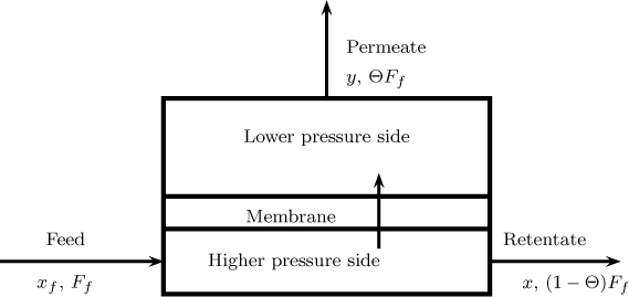
In the membrane process for separation of gas mixtures, the membranes act as a barrier though which some species move faster than others. The feed mixture, usually at a high pressure, is fed to one side of the membrane and is separated into a retentate (part of the feed that does not pass through the membrane) and a permeate (part of the gas that has passed through the membrane). The permeate side is usually at a lower pressure compared to the feed side. A general schematic of a membrane separation process is presented in Figure 27.1. In some cases a sweep gas is fed on the permeate side in order to promote the flow of the permeate. However, this may dilute the permeate stream and cannot be used in some applications.

Gas separation using membranes is employed in a number of industrial applications for separation of gas mixtures. A few examples are indicated here:
Recovery of hydrogen from product streams of ammonia plants, refinery process steams, or mixtures with inert gases such as nitrogen or methane
Enrichment of air to produce oxygen for medical or metallurgical purposes or use in oxidation processes in chemical industries
Removal of CO2 and/or H2S from natural gas
27.1.1 Membrane Classification
There are a number of ways to classify membranes. The usual classification for gas separation is based mainly on the pore size, and membranes can be porous versus non-porous.
Polymers in a glassy state are examples of non-porous membranes. A solution–diffusion model is used as the mechanism of transport in such membranes. The transport rates of different gases are then determined by the differences in their solubility and diffusivity, as discussed later in this section. Since diffusivity in a non-porous matrix is low, the transport rate is low, but selectivity can be high due to solubility differences between the gases in the membrane. Hence the selection of membranes is often a compromise between the rate of transport and the selectivity to a specified gas. Examples of common polymeric membranes include cellulose triacetate, polyisoprene (natural rubber), polycarbonates, polysulfones, and teflon.
Porous membranes are more commonly used for gas separation. The pore diameter must be smaller than the mean free path of gas molecules. Thus the pore size has to be on the order of 10 nm or so. Gas flux through a porous membrane is much higher (three to five orders of magnitude) than for the non-porous case, but the separation selectivity is lower since both gases become closely permeable.
Membranes can also be asymmetric. This represents a compromise between a non-porous and a porous membrane. Here a dense but thin non-porous layer is bonded to a microporous layer. The dense layer provides the selectivity while the porous layer provides increased structural strength.
Although polymeric membranes are common, in special cases materials other than polymers can be utilized. Microporous α-alumina is one example. A second example is the palladium membranes that permit transport solely of hydrogen. Hydrogen is strongly adsorbed over Pd in a dissociative manner and hence the selectivity of such membranes toward hydrogen is very high. The operating temperatures of such inorganic membranes are higher than polymeric membranes.
27.1.2 Transport Rate: Permeability
Consider a membrane of thickness L with a concentration of the diffusing solute of CA0 at x = 0 and CAL at x = L as shown in Figure 27.2.

Figure 27.2 Concentration profiles of A across a membrane; note the concentration jump across the interface.
We can use the Fick’s law type of model for transport across the membrane itself:
where NA is the flux of the diffusing species across the membrane. Note that the low flux mass transfer model used here and NA is assumed to be the same as the Fick’s law flux. DA is the diffusion coefficient of A in the membrane, which is assigned a constant value.
Here CA0 and CAL are the concentration on the membrane side of the interface. This concentration is usually not directly known. What is known is the concentration in the fluid phase on either side of the membrane. The concentration in the fluid is related to the concentration in the membrane by an equilibrium relationship, Thus if CA0,G is the concentration in the gas at x = 0 then the concentration in the membrane CA0 is given as
where KA is an equilibrium solubility constant, also called the partition coefficient. A similar equation holds at x = L. Hence
Using these equilibrium relations in Equation 27.1, we obtain the flux in terms of the concentration driving force based on the fluid concentrations:
Hence the overall transport rate depends on the product of D and K (as well as the thickness L) and not merely on the value of the diffusion coefficient. This composite parameter DK is defined as the permeability of the membrane. This has units of m2/s, similar to that of diffusivity, but it includes the partition coefficient as well.
The driving force can also be based on partial pressure units and a permeability PM,A can be defined by the following equation:
where ΔpA is the partial pressure difference across the membrane. The permeability defined in this manner has units of mole – m/m2 s Pa this case. The two are related by
Barrer
The unit of permeability as defined above is mole – m/m2 s Pa. However, in membrane-related publications, the permeability is often reported in units of barrer, defined as follows:
one barrer = 10–10 cm3 STP. cm/cm2 s Hg – cm
The conversion factor to traditional SI units is as follows:
one barrer = 3.348 × 10⁻¹⁶mole – m/m2 s Pa
The barrer unit is named after early work by Barrer (1951, 1984) in this area. One reason for the persistence of this unit is that the permeability for many membranes is on the order of 1 to 10 barrer and hence the values can be easily remembered. Typical values are shown in Table 27.1 from more extensive data provided by Seader et al. (2011).
Table 27.1 Permeability in Barrer of Common Gases in Typical Membranes at 25 °C
|
H2 |
O2 |
N2 |
CO2 |
Polyethylene |
9.8 |
2.93 |
0.97 |
12.66 |
Polymethacrylate |
– |
1.18 |
0.23 |
5.05 |
Polyvinlchloride |
1.73 |
0.046 |
0.12 |
0.16 |
Butyl rubber |
7.24 |
1.30 |
0.32 |
5.19 |
27.1.3 Transport Rate: Permeance
Usually the thickness of the membrane L is also not precisely known. The partition coefficient K also may not be usually measured and thus may not be known as well. Hence the effects of these terms are combined into an overall term called the permeance of the membrane:
The transport rate across the membrane can thus be described (in terms of the fluid phase concentration difference as the driving force) as
Note that the permeance has the same units as the mass transfer coefficient (m/s) and is hence a measure of transport efficiency of a membrane. The driving force is also defined in this equation in terms of the gas phase concentration difference. The superscript (C) on permeance is used to indicate this.
The permeance of a membrane is a composite parameter that depends on the diffusion coefficient of the membrane itself, the solubility or the partition coefficient of the solute in the membrane, and finally the thickness of the membrane itself. Thus the values of may vary from one type of membrane to another and cannot be correlated in a theoretical sense unless all three effects can be quantified separately. However in practice the permeance is often used to describe the transport rate and in membrane module analysis as a matter of convenience. Often the permeance values are directly reported in the literature, since they can be directly calculated from the measured rate data.
The partial pressure difference is often used in Equation 27.7 instead of the concentration difference. The flux is given as
where A (with no superscript) is now based on the partial pressure difference. The permeance has units of mol/m2.s.Pa (or mol/m2.s.atm if the pressure is expressed in atm). The units are the same as kG, the gas-side mass transfer coefficient used in absorption studies. We will use this definition and the partial pressure difference as the driving force for local flux calculation in permeator scale modeling in Section 27.3.
The effect of temperature is to increase permeance. An increase in temperature causes an increase in diffusivity while the effect of solubility may act in either direction. Overall, a modest increase in permeance with temperature is observed.
27.1.4 Selectivity
The relative rate of transport of two gases is the measure of the selectivity of the membrane to one gas relative to the second. Hence it is useful to define a selectivity parameter, S12 as follows:
or
Thus selectivity depends on both the solubility ratio and the diffusivity ratio.
27.1.5 Sievert’s Law: Dissociative Diffusion
Gases such as hydrogen can dissociate into H atoms in inorganic membranes with noble metals such as Pd and in such cases a nonlinear transport model with a square root dependency is used:
This equation is called Sievert’s law and describes hydrogen transport in Pd-based membranes. The square root dependency arises due to the law of mass action: the concentration of H atoms (the diffusing species) is proportional to the square root of H2 concentration.
27.1.6 Nonlinear Effects in Membrane Transport
The discussion in Section 27.1.2 was based on the simple Fick’s law concept based on constant values of solubility and diffusivity. However, complexities in the transport law often arise due to local differences in both solubility and diffusivity, both of which can be functions of concentration. Stern (1994) made the following classifications:
Constant diffusion and constant Henry’s law (K): This is the simplest case and the model in subsection 27.1.2 is applicable. Diffusion of permanent gases in elastomers and many harder polymers are often described by such a model.
Diffusivity as a function of position: Membranes prepared from composite materials of two or more layers show different values of D for each layer.
Concentration-dependent diffusivity D but constant K: This phenomena is exhibited by gases with critical temperatures near the ambient to 200° C, for example, C4 hydrocarbons in rubbery membranes.
Variable D and variable K: Gases with high critical temperatures, organic vapors, and so on, are examples of systems showing this pattern.
Time-dependent effect, that is, D(CA, t): Here a time- and history-dependent diffusion phenomena is observed. These are seen in polymers with longer relaxation times, for example, organic vapor in ethyl cellulose.
Further discussion of these complex effects is not considered here. The main point is for you to be aware of these phenomena in practical applications and use specific modifications in the model as needed. The models for all the preceding cases can be set up using the methodology described in Chapter 6 for variable diffusivity problems. Numerical computation is usually needed to integrate the local model across the membrane thickness.
Dual Mode Transport
Another model that shows a nonlinear dependency is the dual mode transport model first proposed by Barrer et al. (1958) and then by Koros and Paul (1980). The model is useful for rubbery polymers. In this model, the solution is determined by using Henry’s law (linear) in the polymer chains and by the Langmuir isotherm (nonlinear) in holes or sites between chains of glassy polymers. The overall permeance is a weighted average of the linear and nonlinear part of the solution–diffusion model for the two sites. For further details consult the mentioned references.
27.2 Gas Translation Model
The gas translation model, also called the activated Knudsen model, is often used to calculate the permeance and the selectivity parameter. A brief overview of this model is given here. The model was first developed by Xiao and Wei (1992) and later modified by Shelelkhin et al. (1995) and Nagasawa et al. (2014). The model is applicable to microporous membranes where diffusion is the main controlling parameter. The partition coefficient is not much different for many gases in such membranes (unlike polymeric membranes) and hence the selectivity depends mainly on the diffusivity in this case. (The partition coefficient K will be taken as one in the following discussion.)
The gas translation model can be viewed as an extension of the Knudsen diffusion concept. In small micropores the pore diameter is smaller than the molecular mean free path and hence diffusion is through the Knudsen mechanism. Note that the Knudsen diffusion coefficient in a cylindrical straight pore (Section 7.5.1) is given as
where dp is the diameter of the pore. The term within the square root is the mean free path of the diffusing gas.
The corresponding permeability is given by using the porosity and a tortousity factor:
The gas translation model is a modification of the above relationship, which was based on the Knudsen diffusion concepts. In this model, the permeate diffusion is assumed to be restricted from the potential field of the membrane wall and a correction factor, pi, is applied to the this formula. The permeabiity equation is then multiplied by the following factor:
The factor pi represents the probability factor, which represents the fraction of molecules that have the energy to overcome the activation barrier; this is modeled by an Arrhenius type of equation:
p0 is the pre-exponential factor and Ei is the activation energy barrier for transport through the pores.
The concepts behind the modified gas translation model are shown in Figure 27.3. Since the center of the permeating molecules cannot approach the pore wall, the effective cross-sectional area is modeled as a circle with a diameter equal to the effective diffusion length dp – dA, as shown in this figure.

Figure 27.3 Schematic of membrane permeation in a pore and effect of size of the permeate molecule. From Nagasawa et al. 2014.
dA is the effective molecular diameter of species A. The ratio of this area to the physical area is used as the pre-exponential factor: hence the pre-exponential factor, p0, is modeled as
Introducing this into Equation 27.10, the permeability can be written as
This provides a useful expression to correlate data on the various gases in terms of structural parameters and an activation energy parameter.
The model also provides a way to assess the selectivity parameter for two gases based on the gas properties. Taking the ratio of the permeability for two gases, the selectivity parameter is given by
d1 and d2 are the molecular diameters of species 1 and 2 respectively. This equation indicates a dependency on the molecular size as well in addition to the molecular weight. The Knudsen model would have predicted only the effect of molecular weight. The second difference is in the temperature effect. The classical Knudsen predicts a square root relation while the gas translation model predicts an additional exponential effect. Thus the temperature dependency is
27.3 Gas Permeator Models
Here we focus on modeling at the equipment level. Membrane separation systems are often modeled based on idealized flow patterns. Four common patterns are shown in Figure 27.4.

Figure 27.4 Four idealized flow patterns in membrane separation unit. Based on Seader, J. D. Henley, E. J. and Roper D. K. (2011). Separation Process Principles with Applications using Process Simulators, John Wiley & Sons, Hoboken, NJ.
Basic aspects and useful relations common to all four models are first presented. A binary feed consisting of A and B is considered.
The following notation is used here: x is the mole fraction of A in the retentate and y is the mole fraction of A in the permeate (i.e., species subscript A is dropped.) These are also local values at any position in the bulk gas.
27.3.1 Flux Relations
The flux across the membrane is represented as
where P1 is the pressure on the membrane side and P2 is the pressure on the pemeate side. A is the permeance of species A.
Similarly for B the flux is given as
The pressure ratio parameter and selectivity parameter are introduced to simplify the above equations.
The selectivity parameter is defined as
The pressure ratio parameter is defined as
With these definitions, the fluxes are given as
27.3.2 Local Concentration
It is useful to define a local mole fraction y′ in the permeate side. This definition is useful to set up mass balances on the permeate side:
Using the fluxes the following relation can be shown for the local permeate composition, y′:
This equation provides the local composition of A crossing the membrane and it can then be used to model the performance of a membrane separator. The material balance equations are to be coupled with these flux relations. The material balances are different for different flow patterns as shown in Figure 27.4. Hence the effect of flow patterns needs to be accounted for; these are studied next.
Before we show these details of permeator performance calculations, it is worth noting two limiting cases of Equation 27.16. The first is when P* equal to zero. This will give the maximum local mole fraction in permeate:
The second limiting case is when P* = 1. The value of y′ is now zero since there is no driving force for diffusion when the pressures are equal on both sides. Separation is now possible only by adding a third component on the permeate side, which is called the sweep gas. This is used in some applications to improve separation. However, the sweep gas dilutes the permeate gas and hence may not be suitable in some applications.
There is also a minimum value of P* that is independent of the value of S. This arises due to the requirement that the partial pressure of A in the permeate does not exceed that in the feed:
P1xf ≥ P2ymax
Since ymax can not exceed one, the operating pressure ratio has to be less than the following minimum value:
P* ≤ xf
For example if the feed is 40% A, the pressure ratio has to be less than 0.4 in order to get a nearly pure A (in the permeate stream) under ideal operating conditions. This is similar to the minimum reflux concept in distillation operation. Here we have a minimum retentate side pressure criteria.
Gas permeator models are considered next. We examine the simplest case (backmixed-backmixed) first.
27.3.3 Backmixed-Backmixed Model
Here we provide a simple model to evaluate the performance of a gas permeator. The model assumes the gas is well mixed on both the high and low pressure side. The basis of the model is shown schematically in Figure 27.5.
The following notation is used in this section: Ff is the molar flow rate of the feed with xf the mole fraction of A in the feed. x is the exit mole fraction in the retentate; y is the exit mole fraction on the permeate side. Due to the assumption of complete mixing on the permeate side, the mole fractions x and y are also representative of the mole fractions in the permeater itself.
It is customary to use a cut parameter, denoted as Θ. This is defined as the fraction of the feed that becomes the permeate:
Here Fp is the permeate molar flow rate.
The mass balance for A gives
This can be expressed using the cut parameter and rearranged to give
This has the status of an operating line since it is based on mass balance and relates x to y. A second relation between these two is given by transport considerations, which are shown next.
The mole fraction in the retentate side y is now equal to the local mole fraction y′ since there is no other flow in the retentate (no sweep gas). Hence Equation 27.16 relates y and x. This is reproduced below with the left-hand side changed to y now:
Equations 27.18 and 27.19 can be solved simultaneously to find the exit mole fractions for a given feed mole fraction with the cut as a parameter. Additional parameters to be specified are the selectivity ratio S and the pressure ratio P*. Since the cut varies from 0 to 1, a design type of plot can be constructed for the permeate mole fraction as a function of the cut. An illustrative plot of membrane performance is shown in Figure 27.6.

Figure 27.6 Membrane performance as a function of the cut parameter. xf = 0.21, S = 1000, P* = 100. Backmixed-backmixed model.
The model is useful for laboratory studies to interpret data and to evaluate permeability values as these are often operated such that the back-mxied assumption is reasonably valid.
The transfer area needed can then be calculated from the following equation:
This will provide a conservative estimate since the driving force will be larger in other flow patterns. The flow pattern examined next is the counterflow of the two streams.
27.3.4 Countercurrent Flow
A common mode of operation is the hollow fiber permeater. A schematic of this is shown in Figure 27.7.
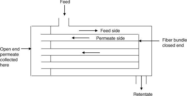
Here the membranes are made in tubes or fibers and tied together to form a bundle. The fiber bundle is put into a shell where the feed stream is contacted. The species diffuse into the fiber and the permeate is collected at the open end as shown in the figure. The flow is usually countercurrent since it provides a better degree of separation compared to cocurrent flow. A model for performance analysis is presented in this section.
A differential model is called for since the mole fractions vary along the tube length. However, if the differential model is discretized (e.g., by an implicit Euler scheme) an equivalent stagewise representation is obtained and can be used to simulate the process. A schematic of this is shown in Figure 27.8. The model equations are the species balance and the total flow balance for the permeate and the feed side; these are presented next. The permeater is divided into N stages with stage 1 starting at the closed end of the system. Each stage is assumed to provide an area ΔAm for mass transfer.
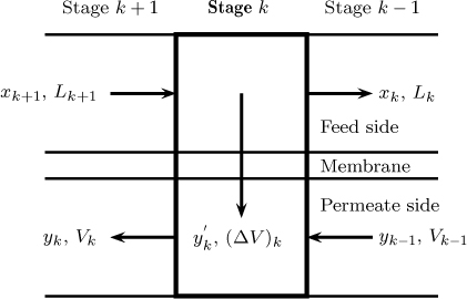
Figure 27.8 Model notation for stagewise computation of a membrane separator with countercurrent flow. Note ΔV is the permeation mole flow and is equal to JA + JB.
The following notation is used: L is the molar flow rate on the feed side and V is the flow rate on the permeate side. The subscript will be used to denote the stream leaving a stage. The stream entering a stage will have the subscript of the stage from where it came. This notation is similar to that used in distillation. The balance equations using this notation are presented next.
The species balance on the feed side can be derived as
Lk+1xk+1 – Lkxk = (JA + JB)y′kΔAm
The total balance on the feed side is
Lk+1 – Lk = (JA + JB)ΔAm
The following equation holds for the species balance on the permeate side:
Vk–1yk–1 – Vkyk = –(JA + JB)y′kΔAm
Finally, the total balance is needed for the permeate side:
Vk–1 – Vk = –(JA + JB)ΔAm
y′k and xk are related by Equation 27.16.
A simple solution procedure is as follows. The computations are usually started at the closed end since the permeate conditions can be specified at this end. The retentate flow and mole fraction are assumed at this end. This is stage one. Hence L1 corresponds to the specified (or guessed) retentate flow and x1 is the mole fraction at the exit. For the permeate, V0 and y0 are zero in the absence of the sweep gas. All the quantities for starting the calculation for stage one are therefore known and the composition and flow leaving stage one can now be calculated. These are then used for the next stage and we can move across the system to end up in stage N.
What value should be assigned to the number of stages N? This depends on whether it is a simulation or design problem. If it is a simulation problem the total area for mass transfer Am is known. We can discretize this to any number of stages. The larger N is, the more accurate the results (with more computations) since the differential model is now closely approached. The parameter ΔAm has to be selected as Am/N and will depend on the value of N chosen. The calculations are done for N stages and provide the values for the inlet feed conditions and also the exit permeate flow and mole fraction for the chosen exit retentate conditions. Using many different exit conditions, a design chart (a parametric plot) can be prepared.
For a design problem a value of ΔAm is chosen as an incremental area for simulation. The stagewise calculations are continued until the inlet feed mole fraction is reached. This provides the number of stages (N) needed to achieve the separation. The required membrane area is then calculated as N ΔAm.
Effect of Pressure Variation
The model shown above assumed that the pressures are constant on both the feed and permeate side. Hence the pressure ratio does not vary across the permeater. A rigorous analysis should include the pressure variations in the feed and permeate sides due to frictional losses. The feed is usually in the shell side in the hollow fiber type of arrangement. The pressure drop on the shell side is usually small and no significant error is caused by assuming that the pressure in the shell is a constant. For the permeate side the pressure gradient is zero at the closed end and increases gradually as we approach the discharge end. The pressure variation can be included in the stagewise model by computing the pressure drop in each stage based on the local velocity at that stage. Note the pressure drop depends on the permeate flow rate at each stage and cannot be assigned a priori. Hence this represents a problem where the momentum transfer is coupled to mass transfer.
The analysis of the cocurrent flow pattern shown in Figure 27.4 involves merely switching the flow arrangement in Figure 27.8 and is not presented here.
27.3.5 Cross-Flow Pattern
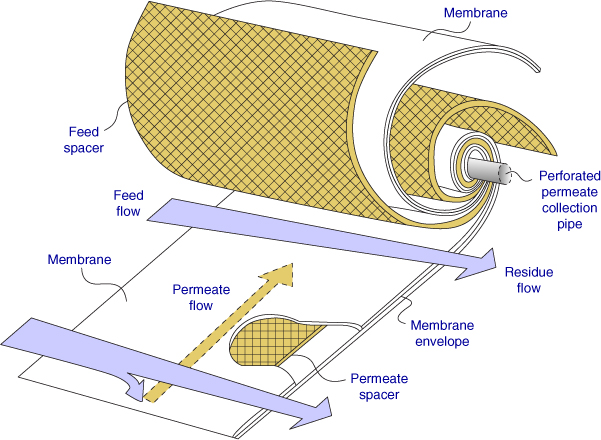
Another contacting pattern is the cross-flow. The fibers are often spiral wound with a center pipe as the permeate collector. The feed and the permeate flow in a cross-flow manner as shown in Figure 27.9.
A stagewise model is useful and is shown in Figure 27.10.

Figure 27.10 Model notation for stagewise computation of a membrane separator with crosscurrent flow.
The permeate from each stage is assumed to flow into the center pipe. The model is merely a simplification of the countercurrent flow. The V terms in the permeate balance are set as zero. Stage k contributes a permeate molar flow of (ΔV)k, which is equal to JA + JB from that stage. The composition of this stream is the same as the local composition y′. Hence yk = y′k is used in the feed species balance equations. The total permeate flow is the sum of the flow from the N stages and the composition is the weighted average:
27.4 Reactor Coupled with a Membrane Separator
This section presents an example of a reactor-separator combo. The walls of the reactor are selectively permeable to a product or reactant. The product removal, for example, overcomes the limitation of an otherwise equilibrium-limited reaction. The arrangement therefore provides a more compact design plus greater conversion. Removal of a product increases the residence time for a given volume of reactor and drives equilibrium-limited reactions toward completion. Another advantage is that the operating range of temperature and pressure is larger.
A schematic of a membrane reactor with product removal is presented in Figure 27.11. One widely studied example is the steam reforming of methane to produce synthesis gas:
CH4 + H2O ⇌ 3H2 + CO

The reaction is endothermic and equilibrium limited. The water gas shift reaction also occurs in parallel:
CO + H2O ⇌ H2 + CO2
This reaction is mildly exothermic. The simultaneous removal of hydrogen shifts the equilibrium to the right. Also it is possible to operate the reactor at somewhat lower temperature.
A second example is the cracking of cyclohexane to benzene:
C6H12 ⇌ C6H6 + 3H2
Again equilibrium limitations can be overcome by the use of a membrane reactor. Hydrogen-selective membranes that operate at high temperatures are used in these processes.
Another potential application is in partial oxidation. Here one of the reactants (oxygen) is introduced into the reactor by transport across a membrane. The membrane provides a means of supplying oxygen to the system at a controlled rate. The concentration of oxygen can be adjusted (usually to a low value) so that the secondary oxidation reactions are suppressed. A schematic of a membrane reactor with reactant dosing is shown in Figure 27.12.

Summary
Membrane-based processes and separations are becoming important in a number of industrial applications and an engineer should be able to analyze and evaluate these processes. Membranes are of course of importance in biological transport in cells and other organs as well.
For separation of gaseous mixtures, polymer-based membranes are most commonly used. These are essentially non-porous and hence the rate of transport is governed by dissolution accompanied by diffusion. A second class of membranes is nano-porous materials with pore size comparable to the mean free path. In view of the small size of these pores, the Knudsen diffusion is often the operating mechanism in these systems.
Membranes for gaseous separation in polymeric membranes can be modeled on the basis of the solution-diffusion model. The transport rate is based on the permeability parameter, which is the product of the diffusivity and the solubility divided by the membrane thickness. The relative rate of transport between two gases can be changed by changing the solubility rather than the diffusivity. Thus the solubility parameter plays a key role in the selectivity of the membrane for polymeric membranes.
Hydrogen diffuses in many membranes after dissociation to H atoms. This is important in many Pd-coated high temperature ceramic membranes. If the equilibrium for dissociation is included, the permeation rate is proportional to the square root of the hydrogen partial pressure rather than being linearly proportional. The resulting expression for permeation is known as the Sievert law.
For hydrocarbons in polymeric membranes various nonlinear effects are encountered. This can include nonlinear equilibrium relations, nonlinear concentration dependent diffusivity, and time variation in permeability caused by swelling or viscoelastic effects.
The selectivity for gas separation in microporous membranes is primarily affected by the relative diffusion coefficient ratio. Knudsen diffusion is the main mechanism for diffusion. An improved model is the gas translation model where the Knudsen model is corrected for the diameter of the diffusing species and an activation barrier for pore diffusion.
There are several ways of arranging the membrane and contacting it with the feed and withdrawal of the permeate. This leads to various flow patterns. Permeator models can be developed by combining species balance and accounting for the effect of the flow pattern.
The simplest flow pattern to model is the case where both the feed side and the permeate side are well mixed. There is no spatial variation of y and x in this case. The mole fraction in the exit permeate and retentate can be calculated by solving Equations 27.18 and 27.19 in the text simultaneously. The input parameters needed to find the y–x split are the pressure ratio, the selectivity value, and the cut (fraction of the feed flow removed as permeate). Once the transfer rate is known the transfer area can be calculated from the permeability model. This model is useful for laboratory measurements of membrane permeance and selectivity since the interpretation of data is simple and not influenced by the flow pattern. This is reminiscent of differential reactors used for kinetic measurements.
The membranes are commonly assembled in a hollow fiber arrangement and this is similar to a shell and tube heat exchanger. The flow pattern is usually countercurrent flow in this system. The model is developed using a stagewise model that is similar to the mixing cell model used for reactors. The computations are usually started from the sealed permeate end by assuming an exit retentate flow rate and mole fraction. The calculations are done all the way back to the feed end until the feed composition is reached (design problem) or the prescribed number of stages is reached (simulation problem). This provides the feed flow rate and the cut parameter. The performance (degree of separation) can then be tabulated as a design chart in terms of the cut parameter for various pressure ratios and selectivity values.
Pressure drop variations (mainly on the permeate side) can be included in the stagewise model by calculating the frictional pressure drop for each stage. This depends on the permeate velocity in each stage.
Cross-flow is another flow pattern. This is encountered for instance in spiral wound membranes and in radial flow type of arrangements. A stagewise model is again useful from a computational point of view. The local mole fraction is representative of the permeate mole fraction in each stage and the exit mole fraction is calculated as the weighted average of the flow times the mole fraction from each stage.
Reactors can be combined with membrane separators to go beyond equilibrium conversion with selective removal of product. This is mainly used when hydrogen is the product. Membranes can also act as a controlled feed for a reactant; this is useful to control the selectivity of partial oxidation reactions.
Review Questions
27.1 What are the two streams from a membrane separator called?
27.2 What is meant by a sweep? When is it used?
27.3 What is a barrer?
27.4 What is the effect of temperature on the permeability?
27.5 State Sievert’s law. Where is it used?
27.6 State factors that could lead to nonlinear models for membrane transport.
27.7 What are the assumptions in the dual mode transport model in polymeric membranes?
27.8 What additional effects are included in the gas translation model compared to the simple Knudsen diffusion model?
27.9 State four common flow patterns used in membrane separation modeling.
27.10 Define the cut parameter.
27.11 What is the value used for the permeate composition in the cross-flow arrangement?
27.12 State some merits of reactive membranes.
27.13 What is the dosing membrane reactor?
27.14 What is the separating membrane reactor?
Problems
27.1 Permeability units. The permeability of a membrane is reported as 100 barrer. Convert this to permeability based on gas-side concentration driving force and gas-side partial pressure driving force expressed in Pa as well as in atm. If the partition coefficient of the diffusing species is 10, determine the diffusivity in the membrane itself.
27.2 Relative rate based on permeance values. A nitrogen (20%) and methane (80%) mixture is fed to a membrane at a rate of 1000 kmol/hour. The feed pressure is 550 kPa and the permeate is 100 kPa. The permeance values are 50,000 for nitrogen and 10,000 barrer/cm for nitrogen and methane, respectively. Find the flux of each component across the membrane.
27.3 Gas translation model. Estimate the selectivity of hydrogen (dA = 0.25 nm) to nitrogen (0.4 nm) in a membrane with a pore diameter of 0.6 nm. Use the activation energy parameters reported in the paper by Nagasawa et al. (2014) of 4.90 kJ/mole for hydrogen and 7.53 for nitrogen. Compare the values with the selectivity predicted by using the classical Knudsen model. The temperature is 200 °C.
27.4 Permeabilty from differential data. Consider a case where air is separated at a feed rate of 20 L/min with P1 = 3 atm and P2 = 2.6 atm gauge. A 3 L/min STP of permeate with 40% O2 was obtained. The retentate has 17% O2, which is close to the inlet value. Hence an average value for mole fraction can be used for oxygen. Calculate the permeance of oxygen and the selectivity of the membrane for oxygen. A trial and error calculation is needed since the local mole fraction at the permeate side at the inlet is not known. This needs a selectivity value according to Equation 27.16.
27.5 Single-stage separation. Oxygen is separated from air in a membrane that has a selectivity of 8 for oxygen. Determine the maximum separation that can be achieved in a single stage unit. If 60% of oxygen is recovered, find the approximate permeate composition.
27.6 Hydrogen separation. A gas containing 70% hydrogen and the rest methane is separated into a nearly pure hydrogen stream in a counterflow membrane permeator that has a selectivty of 100 for hydrogen. The pressure ratio employed is 0.2. Find the fraction of hydrogen recovered in the permeate if the permeate has a purity of 96% for hydrogen and the cut. Model the separator as a countercurrent flow with ten stages.
27.7 Helium separation from natural gas. Helium has a mole fraction of 0.82% in a natrual gas and a high permeance with a selectivity factor of 200. Find the helium recovery for different cut values. Assume both the permeate and the retentate are close to backmixed flow in the membrane.
27.8 CO2 separation from natural gas. Separation of CO2 from natural gas in a hybrid fixed-site carrier type of membrane has been studied by He et al. (2014). Their data indicate a permeance value of 0.2 m3 STP/m2 hour bar for CO2 and a selectivity in the range of 30. The feed contains 10% CO2 and the retentate should have less than 3% CO2. A countercurrent unit is used and the pressure ratio is 0.3. Suggest a design by specifying a feed cut. Find the permeate composition.
27.9 Recovery of VOC from air. VOC can be separated by using highly selective membrane and Baker et al. (1987) examines this potential. A membrane with permeability of 20,000 barrer for VOC (acetone) and 4 barrer for air was used with a membrane thickness of 2 μm. The feed was 0.5% acetone at atmospheric pressure while a pressure of 3 cm Hg was used in the permeate side. The flow rate was 0.2 m3/min in a spiral wound type of arrangement. Find the membrane area needed if the retentate has 0.05% mole of acetone and the permeate has 5% mole of acetone.