Chapter 8. Transient Diffusion Processes

Search in book...
Toggle Font Controls
Create new playlist

Name your new playlist

Playlist description (optional)
Sign In

Email address

Password

Forgot Password?

or

Continue with Facebook

Continue with Google
Sign Up

Full Name

Email address

Confirm Email Address

Password

or

Continue with Facebook

Continue with Google

Chapter 8. Transient Diffusion Processes

Learning Objectives

After completing this chapter, you will be able to:

Understand and use the separation of variables method for the solution of homogeneous linear partial differential equations.
Use the modified method of separation of variables for non-homogeneous problems.
Understand the superposition method for the solution of multidimensional transient diffusion problems.
Solve transient problems posed on a semi-infinite domain.
Understand the concepts behind the penetration model for mass transfer from a gas–liquid interface.
Solve eigenvalue problems with the CHEBFUN program.
Solve partial differential equations numerically with the PDEPE program in MATLAB.

In Chapter 2 we briefly examined some problems on transient diffusion, albeit on a qualitative basis. In this chapter we examine unsteady state problems in more detail. This chapter introduces and solves such problems and illustrates a number of important mathematical and computational techniques to obtain the solutions.

For linear partial differential equations, analytic solutions based on the direct separation of variables method are commonly used. They can be applied to problems where the differential equations and the boundary conditions are homogeneous (explained in the text) and apply to problems posed in a finite spatial domain. This solution procedure is developed and demonstrated here, focusing more on a physical perspective rather than a rigorous mathematical viewpoint.

The method of separation of variables cannot be used directly for non-homogeneous problems and needs some modifications. We study such problems next and then present a number of examples. A more general solution method is based on the eigenfunction operator and known as the finite Fourier transform method. This can be applied to a wider class of (still linear) problems, but this method is not discussed in this text.

Many problems in transient diffusion are posed on a semi-infinite domain. For such problems a solution method based on similarity transformation is useful. This method is introduced and applications to a number of problems are described. An important application of this is the penetration model for mass transfer, which is often used in lieu of the classical film theory. Another application is to predict the effect of a reaction on mass transfer under transient conditions, which is taken up in detail later in the context of gas–liquid reactions.

For nonlinear problems, numerical solutions are required and we discuss one program based on MATLAB code, PDEPE, as an illustrative and useful method for nonlinear problems.

This chapter therefore provides an introduction to solution methods for transient mass diffusion problems together with some useful worked examples.

8.1 Transient Diffusion Problems in 1-D

The governing equation for transient diffusion follows from the general equation for mass transfer derived in Chapter 5:

\begin{matrix} \frac{\partial C_{A}}{\partial t} + \nabla \cdot N_{A} = R_{A} & (8.1) \end{matrix}

$\begin{matrix} \frac{\partial C_{A}}{\partial t} + \nabla \cdot N_{A} = R_{A} & (8.1) \end{matrix}$

If a low flux mass transfer model is used for N_A, which is then equal to J_A, and if Fick’s law is used for diffusion (with a constant value for D_A), we have:

\begin{matrix} \frac{\partial C_{A}}{\partial t} = D_{A} \nabla^{2} C_{A} + R_{A} & (8.2) \end{matrix}

$\begin{matrix} \frac{\partial C_{A}}{\partial t} = D_{A} \nabla^{2} C_{A} + R_{A} & (8.2) \end{matrix}$

The Laplacian can be simplified for common 1-D problems as presented in Figure 8.1. These problems are 1-D diffusion in a slab, and diffusion only in the radial direction in a long cylinder or sphere. These are important and useful problems and will be analyzed in detail in the following sections. We examine the solutions to these 1-D problems for the cases where the separation of variables can be directly applied. Then we show some cases where a modified method is required.

Diagrammatic representation of one-dimensional diffusion in a slab, cylinder, and a sphere.

Three diagrams are shown. The first one represents one-dimensional diffusion in a slab. The slab is taken projected as a graph, One end of the slab is marked 0 (origin) while the other end is marked L, this edge is the horizontal axis representing x. The vertical axis is the left edge of the slab and it represents Increasing time. At L, concentration C subscript A equals 0, and at the top of the slab, C subscriptAi equals 1. Three decreasing, concave down curves are drawn from three different points on the vertical axis, and all cease at the bottom right of the slab marked L. The second diagram represents one-dimensional diffusion in a cylinder. A vertical line, the axis, is drawn through the geometric center of the cylinder and the center point is marked as 0, the radius of the cylinder is r, the direction of the diffusion is marked around the axis, from left to right. The third diagram represents one-dimensional diffusion in a sphere. A one-dimensional sphere with its great circle drawn is shown. Its center point is marked 0 and the outer circumference is marked R, the direction of diffusion is marked along the central axis.

Figure 8.1 Three simple geometries where the transient problem can be treated in one spatial coordinate (and time).

8.2 Solution for Slab: Dirichlet Case

The problem analyzed in this section is transient diffusion in a porous slab of thickness 2L; it has an initial concentration of C_Ai and is exposed to a concentration of C_As on the surface. No reaction occurs in the slab and the transient diffusion with reaction case is analyzed later in Section 8.5. We will predict the transient concentration profile in the slab. The problem is shown schematically in Figure 8.2 as problem (a). This can be cast as a homogeneous problem and direct separation of variables can be used. The coordinate system is defined such that x = 0 is the midpoint of the slab. This is a mathematical convenience as will become clear during the derivation.

Diagrammatic illustration of transient diffusion with two different examples.

Two diagrams are shown labeled, Problem a and Problem b. Problem a: A square block with its top edge cut off is shown. The left edge is marked x equals minus L and the right edge is marked x equals L, with its center point, marked 0. A vertical dashed line is drawn through its center point. Two dashed, horizontal lines are drawn, at the top and the bottom. The bottom line is labeled C subscript A (t equals 0) equals C subscript Ai. The top line is marked C subscript As, at t equals infinity. Problem b: A square block with its top edge cut off is shown. The left edge is marked x equals minus L and the right edge is marked x equals L. A dashed horizontal line is drawn at the bottom labeled C subscript A (t equals 0) equals C subscript Ai. Another dashed, slanting line is drawn from the left edge to the right edge. The concentration at the top of the line (left edge) is marked C subscriptA1 and the concentration at the bottom of the line (right edge) is marked C subscript A2, with t equals infinity.

Figure 8.2 Schematic of the illustrative slab transient problems analyzed for transient diffusion. Two cases are shown. Problem (a) is solved by direct separation of variables where the same surface concentration exists at both edges of the slab while problem (b), where the two surface concentrations are different, requires some pre-manipulations prior to solution by the separation of variables method.

A variation of this problem, shown as (b) in Figure 8.2, is analyzed later in Section 8.5. Here the surfaces of the slab are exposed to two different concentrations. The solution requires a modification in the separation of variables method by subtracting out the steady state solution.

For the slab case the governing equation is Equation 8.2 using the Laplacian in Cartesian with only x-dependency:

\begin{matrix} \frac{\partial C_{A}}{\partial t} = D_{A} \frac{\partial^{2} C_{A}}{\partial x^{2}} & (8.3) \end{matrix}

$\begin{matrix} \frac{\partial C_{A}}{\partial t} = D_{A} \frac{\partial^{2} C_{A}}{\partial x^{2}} & (8.3) \end{matrix}$

It is useful to put this in dimensionless form, which is discussed next.

8.2.1 Dimensionless Representation

The dimensionless representation begins by defining a scaled concentration and distance:

c_{A} = \frac{C_{A} - C_{A s}}{C_{A i} - C_{A s}}

$c_{A} = \frac{C_{A} - C_{A s}}{C_{A i} - C_{A s}}$

where C_As is the surface concentration, which remains constant with time for the Dirichlet problem. C_Ai is the initial concentration, which is assumed to be uniform here and not a function of the spatial variable, x. The above dimensionless definition makes the initial concentration one. The surface concentration is now zero, which makes the boundary conditions homogeneous. This is an important consideration when using direct separation of variables.

Note: The initial concentration need not be uniform and can be a specified function of position, in which case the average value of the initial concentration has to be used to define the dimensionless concentration.

The dimensionless distance is defined by ξ as x/L. This also makes the distance go from zero to one. These choices for scaling reduce the equation to the following form using the chain rule:

\begin{matrix} \frac{L^{2}}{D_{A}} \frac{\partial c_{A}}{\partial t} = \frac{\partial^{2} c_{A}}{\partial ξ^{2}} & (8.4) \end{matrix}

$\begin{matrix} \frac{L^{2}}{D_{A}} \frac{\partial c_{A}}{\partial t} = \frac{\partial^{2} c_{A}}{\partial ξ^{2}} & (8.4) \end{matrix}$

The time was not made dimensionless as we do not know what the time scales are. However the equation suggests that L²/D_A should be chosen as the reference time to scale all terms equally. Hence the dimensionless time τ is defined as

τ = \frac{t D_{A}}{L^{2}} = \frac{t}{L^{2} / D_{A}}

$τ = \frac{t D_{A}}{L^{2}} = \frac{t}{L^{2} / D_{A}}$

L²/D_A is the reference time, also called the diffusion time as noted earlier in Example 2.5, and is approximately the time for internal gradients to reach a steady profile for a surface change in the concentration. The τ is thus the ratio of the elapsed time to the diffusion time.

The dimensionless version for further analysis is therefore

\begin{matrix} \frac{\partial c_{A}}{\partial τ} = \frac{\partial^{2} c_{A}}{\partial ξ^{2}} & (8.5) \end{matrix}

$\begin{matrix} \frac{\partial c_{A}}{\partial τ} = \frac{\partial^{2} c_{A}}{\partial ξ^{2}} & (8.5) \end{matrix}$

Note that there are no free parameters, which is a characteristic of a well-scaled problem in general.

The boundary and initial conditions are as follows:

At ξ = 0, we have symmetry and hence ∂c_A/∂ξ =0.
At ξ = 1, we use the specified concentration, which makes c_A = 0.
At τ = 0 we assume a specified initial concentration profile: c_A(τ = 0) = c_Ai(ξ) in general. For the case of a uniform starting concentration profile, c_Ai = 1.

The boundary conditions and the differential equation are homogeneous and we can use the separation of variables method directly.

8.2.2 Series Solution

The separation of variables method starts with proposing a solution as a product of separate functions in time τ and distance ξ. It seeks solutions of the following form:

Assumed form of the solution = G(τ) F (ξ)

The time-dependent part can be shown to be exp

(- λ_{n}^{2} τ)

$(- λ_{n}^{2} τ)$ , where λ_n is a constant known as the eigenvalue. (The subscript n is needed since there are many (infinite) values of λ, as shown later.) Hence we seek solutions of the following form:

From of the solution = exp (- λ_{n}^{2} τ) F_{n} (ξ)

$From of the solution = exp (- λ_{n}^{2} τ) F_{n} (ξ)$

Substituting the assumed solution in Equation 8.5 we find that the F function should satisfy the following ordinary differential equation (verify the algebra):

\begin{matrix} \frac{d^{2} F_{n}}{d ξ^{2}} + λ_{n}^{2} F_{n} = 0 & (8.6) \end{matrix}

$\begin{matrix} \frac{d^{2} F_{n}}{d ξ^{2}} + λ_{n}^{2} F_{n} = 0 & (8.6) \end{matrix}$

The boundary conditions for F follow from those for c_A. Hence we use the following homogeneous conditions:

At ξ = 0, dF/dξ = 0.
At ξ = 1, F = 0.

Equation 8.6 and the associated homogeneous boundary conditions constitute an eigenvalue problem. The solution shown next result in the generation of the F functions, which are known as the eigenfunctions.

Eigenvalues and Eigenfunctions

The general solution to Equation 8.6 is

\begin{matrix} F_{n} (ξ) = A_{n} cos (λ_{n} ξ) + B_{n} sin (λ_{n} ξ) & (8.7) \end{matrix}

$\begin{matrix} F_{n} (ξ) = A_{n} cos (λ_{n} ξ) + B_{n} sin (λ_{n} ξ) & (8.7) \end{matrix}$

where A_n and B_n are the integration constants. Now we will evaluate these using the boundary condition.

Use of the symmetry condition at ξ = 0 will lead to B_n = 0. Hence

F_n = A_n cos(λ_nξ)

Use of the condition at ξ = 1 will lead to

\begin{matrix} A_{n} cos (λ_{n}) = 0 & (8.8) \end{matrix}

$\begin{matrix} A_{n} cos (λ_{n}) = 0 & (8.8) \end{matrix}$

A_n cannot be zero as it will lead to a trivial solution. Hence this equation provides us the means to find the values for λ_n. Since the cos function is zero at π/2, 3π/2, 5π/2, and so on, we have many discrete values for λ_n:

\begin{matrix} λ_{n} = (n + \frac{1}{2}) π & (8.9) \end{matrix}

$\begin{matrix} λ_{n} = (n + \frac{1}{2}) π & (8.9) \end{matrix}$

Here n = 0, 1, 2, 3, ..., generating an infinite set of eigenvalues.

The F function is therefore of the form F_n = A_n cos(λ_nξ). These are known as the eigenfunctions, as indicated earlier.

Series Solution

As there are infinite number of eigenvalues for this problem and all these values are justified, a series solution that incorporates all values of n seems logical; we can write the solution as an infinite series:

\begin{matrix} \begin{matrix} c_{A} (ξ, τ) = \sum_{n = 0}^{\infty} A_{n} exp (- λ_{n}^{2} τ) cos (λ_{n} ξ) \end{matrix} & (8.10) \end{matrix}

$\begin{matrix} \begin{matrix} c_{A} (ξ, τ) = \sum_{n = 0}^{\infty} A_{n} exp (- λ_{n}^{2} τ) cos (λ_{n} ξ) \end{matrix} & (8.10) \end{matrix}$

The only thing missing is that the initial conditions are not yet satisfied. The series constants A_n should be chosen to satisfy the initial conditions as shown in the following section.

8.2.3 Evaluation of the Series Coefficient

Using the initial conditions we have

\begin{matrix} c_{A i} (ξ) = \sum_{n = 0}^{\infty} A_{n} cos (λ_{n} ξ) & (8.11) \end{matrix}

$\begin{matrix} c_{A i} (ξ) = \sum_{n = 0}^{\infty} A_{n} cos (λ_{n} ξ) & (8.11) \end{matrix}$

Now, in order to find explicit expressions for A_n, we have to use the orthogonal property of the F function.

First we state the orthogonality property of the eigenfunctions:

\int_{0}^{1} F_{n} (ξ) F_{m} (ξ) d ξ = 0 if n \neq m

$\int_{0}^{1} F_{n} (ξ) F_{m} (ξ) d ξ = 0 if n \neq m$

In our particular case of this problem, we have

\int_{0}^{1} cos ([n + 1 / 2] π ξ) cos ([m + 1 / 2] π ξ) d ξ = 0 if n \neq m

$\int_{0}^{1} cos ([n + 1 / 2] π ξ) cos ([m + 1 / 2] π ξ) d ξ = 0 if n \neq m$

which can be verified using the table of integrals, MAPLE, or MATHEMATICA. But it is useful to note that the orthogonality property is a general property for all the eigenvalue problems of the Strum-Liouville type. If the differential operator is linear and symmetric then the eigenfunctions are orthogonal (with a weighting function), which is a basic property of such operators. Interested students should refer to the book by Ramkrishna and Amundson (1985) on linear operator methods. We now proceed to evaluate the series coefficients.

If we use the orthogonality property of the eigenfunction, then the series unfolds itself and the coefficients can be found one at a time using the following ratio of two integrals:

\begin{matrix} A_{n} = \frac{\int_{0}^{1} c_{A i} (ξ) cos (λ_{n} ξ) d ξ}{\int_{0}^{1} {cos}^{2} (λ_{n} ξ) d ξ} & (8.12) \end{matrix}

$\begin{matrix} A_{n} = \frac{\int_{0}^{1} c_{A i} (ξ) cos (λ_{n} ξ) d ξ}{\int_{0}^{1} {cos}^{2} (λ_{n} ξ) d ξ} & (8.12) \end{matrix}$

This is applicable to any specified initial condition given by c_Ai(ξ). For a particular case of a constant initial concentration c_Ai = 1, the series coefficients are

\begin{matrix} A_{n} = \frac{\int_{0}^{1} cos (λ_{n} ξ) d ξ}{\int_{0}^{1} {cos}^{2} (λ_{n} ξ) d ξ} = \frac{2 (- 1)^{n}}{π (n + 1 / 2)} & (8.13) \end{matrix}

$\begin{matrix} A_{n} = \frac{\int_{0}^{1} cos (λ_{n} ξ) d ξ}{\int_{0}^{1} {cos}^{2} (λ_{n} ξ) d ξ} = \frac{2 (- 1)^{n}}{π (n + 1 / 2)} & (8.13) \end{matrix}$

This completes the solution to the Dirichlet problem in a slab.

The method holds for all similar problems, for example, the other 1-D geometries mentioned in Figure 8.1. The only changes will be in the eigenfunction, eigencondition, eigenvalues, and series coefficient. If expressions for these are derived, the series solution is complete. In fact the solution to a number of homogeneous PDE problems can be represented in series form similar to that given by Equation 8.10 and similar solution steps can be used. Let us return to the slab problem and look at some features of the solution.

8.2.4 Illustrative Results

An illustrative plot of concentration versus distance is presented in Figure 8.3; it is obtained by summing the series up to 50 terms in MATLAB for some selected values of time.

Graphical representation of concentration versus distance for the slab case with Dirichlet boundary condition.

The horizontal axis represents Dimensionless distance, zeta, ranging from 0 to 1 in increments of 0.2. The vertical axis represents Dimensionless concentration , C subscript A ranging from 0 to 1 in increments of 0.1. Five decreasing, concave down curves are drawn across the graph, all of the curves converging at (1, 0). On each curve, approximately 8 to 10 different points are marked using asterisks. The first curve, with dimensionless time, tau equals 0.02, originates at (0, 1), starts decreasing from (0.6, 0.95) and gradually continues to decrease ceasing at (1, 0). The second curve, with tau equals 0.05 also starts at (0, 1), starts decreasing at (0.4, 0.95) and gradually continues to decrease ceasing at (1, 0). The third curve originates at (0, 0.77) with tau equals 0.2 gradually continues to decrease ceasing at (1, 0). The fourth curve starts at (0, 0.37) with tau equals 0.5, continues to decrease ceasing at (1, 0). The fifth curve starts at (0, 0.11) with tau equals 1.0 and continues to decrease ceasing at (1, 0).

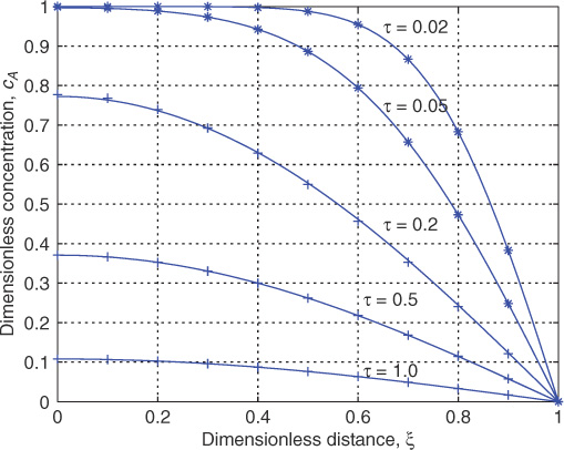
Figure 8.3 Time-concentration plot for slab case with Dirichlet boundary condition at the surface. The points marked * represent the semi-infinite solution for comparison; points marked + show the series solution computed with only one term.

Concentration profiles are rather sharp for small values of τ . The series will converge rather slowly here and a large number of terms is needed. An alternative is to model this as a semi-infinite slab as shown in Section 8.7. The following solution (derived in Section 8.7) will then be applicable:

c_{A} = erf (\frac{1 - ξ}{2 \sqrt{τ}})

$c_{A} = erf (\frac{1 - ξ}{2 \sqrt{τ}})$

where erf represents the error function. This solution is marked as * in Figure 8.3. Note the excellent comparison with the above erf solution for τ < 0.05.

The series converges rapidly for values of τ > 0.2. Only one term may be sufficient to get a reasonable estimate of the concentration profile. Using the term approximation (A₀ = 4/π here) the concentration can be described as a function of time as

c_A = (4/π) exp(–π²τ/4) cos(ξπ/2)

which is valid for τ > 0.2 or so. The one term approximation is marked as + in Figure 8.3 for comparison and we find that this is sufficient for τ > 0.2. Steady state is almost reached around a τ of one. Hence the actual time needed to reach steady state is of the order of the diffusion time, L²/D_A.

The expression for the mass flux at the surface is important in design calculations. This is obtained by applying Fick’s law at the surface. For a constant initial concentration of C_Ai, the expression can be shown to be

\begin{matrix} N_{A s} (τ) = 2 D_{A} \frac{(C_{A i} - C_{A s})}{L} \sum_{n = 0}^{\infty} exp [- (n + 1 / 2)^{2} π^{2} τ] & (8.14) \end{matrix}

$\begin{matrix} N_{A s} (τ) = 2 D_{A} \frac{(C_{A i} - C_{A s})}{L} \sum_{n = 0}^{\infty} exp [- (n + 1 / 2)^{2} π^{2} τ] & (8.14) \end{matrix}$

Students may wish to verify the algebra leading to this expression.

A plot of mass flux as a function of dimensionless time is presented in Figure 8.4. A flux scaled by D_A(C_Ai – C_As)/L is used in this plot. The mass flux is very large at time near zero and decreases with time with square root proportionality in the early stages of the process. At early stages for τ < 0.1, the dimensionless flux can be calculated more simply as $1 / \sqrt{π τ}$ $1 / \sqrt{π τ}$ , which follows from the alternative semi-infinite slab solution shown in Section 8.7. For larger values of time (τ > 0.2 or so), the one-term approximation is sufficient to calculate the fluxes. The flux decreases as an exponential function of time during this period.

Graphical representation shows a plot of mass flux as a function of dimensionless time.

Figure 8.4 Dimensionless mass flux from the surface as a function of time for the slab problem.

8.2.5 Average Concentration

The volume average concentration in the solid is defined in a general manner for all three geometries shown in Figure 8.1:

\begin{matrix} 〈 c_{A} 〉 = (s + 1) \int_{0}^{1} ξ^{s} c_{A} (ξ) d ξ & (8.15) \end{matrix}

$\begin{matrix} 〈 c_{A} 〉 = (s + 1) \int_{0}^{1} ξ^{s} c_{A} (ξ) d ξ & (8.15) \end{matrix}$

where s is the shape factor. Note that ξ^sdξ is a measure of the local volume at any given ξ position.

For the slab case s = 0 and the average concentration is simply the integral under the curve in Figure 8.3 for each time value. The integrated expression is

\begin{matrix} 〈 c_{A} 〉 (τ) = \sum_{n = 0}^{\infty} A_{n} B_{n} exp [- (n + 1 / 2)^{2} π^{2} τ] & (8.16) \end{matrix}

$\begin{matrix} 〈 c_{A} 〉 (τ) = \sum_{n = 0}^{\infty} A_{n} B_{n} exp [- (n + 1 / 2)^{2} π^{2} τ] & (8.16) \end{matrix}$

The term B_n arises from the spatial integration and is given as

B_{n} = \int_{0}^{1} cos (λ_{n} ξ) d ξ = \frac{sin (λ_{n})}{λ_{n}}

$B_{n} = \int_{0}^{1} cos (λ_{n} ξ) d ξ = \frac{sin (λ_{n})}{λ_{n}}$

A related quantity is the fractional mass loss parameter, Φ, which is defined as

Φ = \frac{M_{0} - M (t)}{M_{0}} = 1 - 〈 c_{A} 〉

$Φ = \frac{M_{0} - M (t)}{M_{0}} = 1 - 〈 c_{A} 〉$

This represents the ratio of moles of A that have been removed at the given time to the total amount of moles of A that have to be removed (which is the same as the initial moles in the system $M_{0}$ $M_{0}$ ). An application of the solution is shown in Example 8.1.

Example 8.1 Transient Diffusion of Oxygen

A pool of liquid of 10 cm deep is exposed to air and oxygen diffuses into the pool. Take 1 m² as the surface area. Find the time interval up to which the oxygen concentration is nearly zero at the bottom of the pool. Find the time interval over which the liquid is nearly saturated (90%) with oxygen. For the time equal to half this value, find the oxygen concentration at the bottom of the pool.

The diffusion coefficient of oxygen in water is 2 × 10^–9 m²/s. The saturation solubility of oxygen is found from Henry’s law as 0.27 mol/m³.

Solution

The diffusion time is calculated as (0.1 m)²/[2 × 10^–9m²/s] = 5 × 10⁶ seconds.

From Figure 7.3 we find the concentration at the bottom remains nearly one until about τ = 0.05. Hence this is the time up to which oxygen concentration remains zero at the bottom. The corresponding actual time is 2.5 × 10⁵ seconds.

The time at which oxygen concentration is 90% of the final value corresponds to τ = 1 from Figure 7.3. This corresponds to an actual value of time of 5 × 10⁶ seconds, which is also equal to the diffusion time. A long time is needed to saturate in a stagnant liquid with oxygen and some type of aeration is generally needed to quicken the process.

For half this time (i.e., τ = 0.5) a one-term approximation is sufficient. The dimensionless concentration is

c_A(bottom) = (4/π)exp(–0.5 * π²/4) = 0.3708

For an initial concentration of zero, the definition of c_A is $1 - \frac{C_{A}}{C_{A s}}$ $1 - \frac{C_{A}}{C_{A s}}$ . Using this definition, the actual concentration C_A is calculated as 0.17 mol/m³ for a time of 2.5 × 10⁶ seconds.

8.3 Solutions for Slab: Robin Condition

If the surface is losing mass by convection to the surroundings, the surface concentration is unknown. What we know is the external fluid or ambient concentration, denoted as C_A∞ here. For such problems the convective boundary condition should be used; this is obtained by a balance of mass flux at the surface:

- D_{A} {(\frac{\partial C_{A}}{\partial_{x}})}_{x = L} = k_{m} [C_{A} (at x = L) - C_{A \infty}]

$- D_{A} {(\frac{\partial C_{A}}{\partial_{x}})}_{x = L} = k_{m} [C_{A} (at x = L) - C_{A \infty}]$

The left-hand side is the mass arriving by diffusion while the right-hand side is the mass leaving the surface by convection to the surroundings with k_m defined as the (solid-to-fluid) mass transfer coefficient. The dimensionless temperature c_A is now defined as (C_A – C_A∞)/(C_Ai – C_A∞). The boundary condition in dimensionless form at the surface is

\begin{matrix} (\frac{\partial c_{A}}{\partial ξ})_{ξ = 1} = - B i c_{A} at (ξ = 1) & (8.17) \end{matrix}

$\begin{matrix} (\frac{\partial c_{A}}{\partial ξ})_{ξ = 1} = - B i c_{A} at (ξ = 1) & (8.17) \end{matrix}$

The dimensionless parameter appearing in this boundary condition is Bi, defined as k_mL/D_A. This is known as the Biot number. Thus we have a mixed (Robin) boundary condition with the flux appearing on the left-hand side and the surface concentration appearing on the right-hand side. The surface concentration is no longer constant and varies as a function of time.

Note: C_A∞ assumes that the diffusing solute has a partition coefficient of one in the bulk liquid. Otherwise the term C_A∞ should be replaced by K_AC_A_∞, where K_A is the ratio of the solid concentration of A to its liquid concentration at equilibrium.

The differential equations and the center boundary condition remain the same. The initial condition is taken as unity for further analysis.

The series given by Equation 8.10 is still used but with modified values for eigenvalues, which now are specific to each Biot number. The series coefficients are also different now.

The following relations hold for this case and the student should verify the details:

The eigenvalues are the solutions to the following equation:

$\begin{matrix} B i cos (λ) - λ sin (λ) = 0 & (8.18) \end{matrix}$ $\begin{matrix} B i cos (λ) - λ sin (λ) = 0 & (8.18) \end{matrix}$

Note that the eigenvalues now depend on the Biot number and must be calculated by the solution of this transcendental equation. They are not simple multiples of quantities like π/2 in contrast with the Dirichlet case.
The eigenfunctions F_n are cos(λ_nξ). These functions have the orthogonality property.
The series expansion coefficient for a uniform initial condition of one is

$\begin{matrix} A_{n} = \frac{2 sin (λ_{n})}{λ_{n} + sin (λ_{n}) cos (λ_{n})} & (8.19) \end{matrix}$ $\begin{matrix} A_{n} = \frac{2 sin (λ_{n})}{λ_{n} + sin (λ_{n}) cos (λ_{n})} & (8.19) \end{matrix}$
The expression needed to find the average temperature is the same as before:

$\begin{matrix} B_{n} = \frac{sin (λ_{n})}{λ_{n}} & (8.20) \end{matrix}$ $\begin{matrix} B_{n} = \frac{sin (λ_{n})}{λ_{n}} & (8.20) \end{matrix}$

However, the B_n values are now Biot number dependent since the eigenvalues depend on the value of the Biot number.
An illustrative example of the effect of the Biot number is shown in Figure 8.5.

The horizontal axis represents Dimensionless distance ranging from 0 to 1 in increments of 0.2. The vertical axis represents Dimensionless concentration ranging from 0 to 1 in increments of 0.1. Graph legend reads Biot equals 2. Four decreasing curves are drawn across the graph. The first curve, with dimensionless time, tau equals 0.2, originates from (0, 0.92) and ceases at (1, 0.45). The second curve with tau equals 0.4, originates from (0, 0.74) and ceases at (1, 0.35). The third curve with tau equals 1.5, originates from (0, 0.23) and ceases at (1, 0.11). The fourth curve with tau equals 5.00, originates from (0, 0.12) and ceases at (1, 0.05). All coordinate values are approximate.

Figure 8.5 Time-concentration plot for the slab case with a Robin boundary condition at the surface. A Biot number of two is used in this illustration.

Two limiting cases are noted below:
- – For large Bi (> 20), the eigenvalues reduce to λ_n = (n + 1/2)π and the Dirichlet solution is recovered for large Bi. The physical interpretation is that the surface concentration becomes nearly the same as the bulk concentration.
- – For small Biot numbers (Bi < 0.3), a lumped parameter approximation is sufficient. The physical interpretation is that there is no significant internal concentration gradient and the external mass transfer rate becomes the limiting factor. An overall macroscopic mass balance for the solid is sufficient here. The volume-averaged concentration predicted by such a model is
  
  $\begin{matrix} < c_{A} > = exp (- B i τ) & (8.21) \end{matrix}$ $\begin{matrix} < c_{A} > = exp (- B i τ) & (8.21) \end{matrix}$

Derivation of the lumped parameter model is left as en exercise. Drying a porous solid is an example where such a model is likely to apply because the external partial pressure difference in the gas phase is the limiting driving force.

8.4 Solution for Cylinders and Spheres

The solution for cylinders and spheres can be obtained using the same procedure. The series solution can be represented as

\begin{matrix} c_{A} (ξ, τ) = \sum_{n = 0}^{\infty} A_{n} exp (- λ_{n}^{2} τ) F_{n} (λ_{n} ξ) & (8.22) \end{matrix}

$\begin{matrix} c_{A} (ξ, τ) = \sum_{n = 0}^{\infty} A_{n} exp (- λ_{n}^{2} τ) F_{n} (λ_{n} ξ) & (8.22) \end{matrix}$

where λ_n are the eigenvalues and F_n is the corresponding eigenfunction. The expressions for these and the series coefficient for long cylinders and spheres are given in the following subsections without derivation.

Note: The coefficient A₀ = 0 for cylinders and spheres and the above series starts with n = 1.

8.4.1 Long Cylinder

The solution for a cylinder is in terms of the Bessel functions of the first kind and can be enumerated as follows:

The eigenvalues are the solutions to

BiJ₀(λ) – λJ₁(λ) = 0

The values can be found by the solution of the above nonlinear equation for λ for a fixed Biot number.
The problems with large values of the Biot number are often of more interest in mass transfer problems because the internal diffusion is often rate limiting compared to external mass transfer. For this case the eigenvalues can be directly found as the roots of

J₀(λ) = 0

The first three eigenvalues are 2.4048, 5.5201, and 8.6537 from tabulated or calculated values of the J₀ Bessel function.
The eigenfunctions F_n are J₀(λ_nξ).
The eigenfunctions are orthogonal to each other with a weighting factor of ξ.
The series expansion coefficient for a uniform initial condition of one is

$A_{n} = \frac{2 J_{1} (λ_{n})}{λ_{n} [J_{0}^{2} (λ_{n}) + J_{1}^{2} (λ_{n})]}$ $A_{n} = \frac{2 J_{1} (λ_{n})}{λ_{n} [J_{0}^{2} (λ_{n}) + J_{1}^{2} (λ_{n})]}$

Note that the series coefficients simplify for the large Biot case to

$A_{n} = \frac{2}{λ_{n} [J_{1} (λ_{n})]}$ $A_{n} = \frac{2}{λ_{n} [J_{1} (λ_{n})]}$
The coefficients B_n needed to calculate the average concentration are

$B_{n} = 2 \frac{J_{1} (λ_{n})}{λ_{n}}$ $B_{n} = 2 \frac{J_{1} (λ_{n})}{λ_{n}}$

8.4.2 Sphere

The eigenfunctions for a sphere belong to a class of Bessel functions of the spherical kind. The results are as follows:

The eigenvalues are the solutions to the following transcendental equation:

λ cos(λ) + (Bi – 1) sin(λ) = 0
For the large Biot number case, the eigenvalues can be directly found as the roots of

sin(λ) = 0

Hence the first two eigenvalues are π and 2π.
The eigenfunctions F are sin(λξ)/(λξ).
The eigenfunctions are orthogonal with a weighting factor of ξ².
The series expansion coefficient for a uniform initial condition of one is

$A_{n} = \frac{sin (λ_{n}) - λ_{n} cos λ_{n}}{λ_{n} - sin (λ_{n}) cos (λ_{n})}$ $A_{n} = \frac{sin (λ_{n}) - λ_{n} cos λ_{n}}{λ_{n} - sin (λ_{n}) cos (λ_{n})}$

The series coefficients simplify for the large Biot case to

$A_{n} = \frac{2}{cos (λ_{n})}$ $A_{n} = \frac{2}{cos (λ_{n})}$
The coefficient needed to find the average concentration is

$B_{n} = 3 \frac{\sin (λ_{n}) - λ_{n} cos (λ_{n})}{λ_{n}^{3}}$ $B_{n} = 3 \frac{\sin (λ_{n}) - λ_{n} cos (λ_{n})}{λ_{n}^{3}}$

Note that the above coefficient simplifies for the large Biot case to

$B_{n} = - 3 \frac{cos (n π)}{n^{2} π^{2}}$ $B_{n} = - 3 \frac{cos (n π)}{n^{2} π^{2}}$

An illustrative plot of the concentration profile for a sphere with the Dirichlet condition is shown in Figure 8.6. Note that a nearly steady state value is attained for dimensionless time of τ = 0.3. Also, for τ > 0.1 a one-term approximation discussed in Section (8.4.3) is sufficient.

The horizontal axis represents Dimensionless distance, zeta, ranging from 0 to 1 in increments of 0.2. The vertical axis represents Dimensionless concentration, C subscript A, ranging from 0 to 1 in increments of 0.1. Five decreasing curves are drawn across the graph, with several points plotted on or along them with asterisks. All the curves converge at (1, 0). The first curve with dimensionless time tau equals 0.02, originates from (0.3, 1) and gradually decreases to cease at (1, 0). The second curve with tau equals 0.05 originates at (0, 0.96) and gradually decreases to cease at (1, 0). The third curve with tau equals 0.1 originates at (0, 0.71) gradually decreases to cease at (1, 0). The fourth curve with tau equals 0.2, originates at (0, 0.27) gradually decreases to cease at (1, 0). The fifth curve with tau equals 0.3, originates at (0, 0.1) gradually decreases to cease at (1, 0).

Figure 8.6 Time-concentration plot for transient diffusion in a sphere with Dirichlet boundary condition at the surface. The points marked * represent the semi-infinite solution for comparison; points marked + show the series solution computed with only one term.

The surface flux calculated for the sphere problem is presented in Figure 8.7, which shows the effect of Biot number. This represents a case where there is a barrier to diffusion near the surface, for example, having an inert core near the surface. The flux is reduced at lower Biot numbers as expected, but the release rate is more uniform. In other words a large rate at times near zero, a characteristic of the Dirichlet problem, is no longer observed. This has implications on the design of drug capsules which can provide a nearly uniform release rate.

Graphical representation of the surface flux calculated for the sphere problem.

Figure 8.7 Effect of Biot number on the instantaneous flux from a sphere; in the simulation Biot = 1.33. Flux is dimensionless and a scale flux of D_AC_Ai/R is used as a reference. Note that the release rate has become somewhat more uniform due to the diffusion barrier.

8.4.3 One-Term Approximation

Often the leading term of the series is accurate enough for large values of time, τ > 0.1 for spheres and 0.3 for slabs. This is known as the one-term approximation. Often we are interested in the concentration at the center as the response is slowest at this point. The one-term approximation for the center concentration is

c_{A} (ξ = 0) \approx A_{1} exp (- λ_{1}^{2} τ)

$c_{A} (ξ = 0) \approx A_{1} exp (- λ_{1}^{2} τ)$

Similarly the average temperature is another quantity of interest; the one-term approximation for this is

〈 c_{A} 〉 \approx A_{1} B_{1} exp (λ_{1}^{2} τ)

$〈 c_{A} 〉 \approx A_{1} B_{1} exp (λ_{1}^{2} τ)$

Note that the average concentration is equal to the center concentration multiplied by B₁. Only the first eigenvalues and the first series coefficients are needed for the one-term model. Further the large Biot case is of interest in mass transfer processes. The values of the parameters needed in the one-term approximation for this Dirichlet problem are shown in Table 8.1; they are for quick calculation for design purposes. The following problem shown in Example 8.2 illustrates the use of the one-term approximation.

Table 8.1 Coefficients for use in the One-Term Approximation. Large Biot Number Case.

–	$λ_{1}^{2}$ $λ_{1}^{2}$	A₁	B₁
Slab	2.467	1.273	0.6366
Cylinder	5.784	1.602	0.4317
Sphere	9.869	2.000	0.3040

Example 8.2 Drug Release Rate from a Capsule

A capsule has a radius of 0.3 cm and has an initial drug concentration of 68.9 mg/cm³. The diffusion coefficient of the drug in the porous matrix is 3 × 10^–6 cm²/s. Calculate and plot the center concentration and the amount of drug released as a function of time. Use one-term approximation as a simplification, but note in general that this is not valid for short times.

Solution

First we estimate the time constant to calculate how long the process will last:

Time constan = \frac{R_{2}}{D_{A}} = \frac{({0.3}^{2}) {cm}^{2}}{3 \times 10^{- 6} {cm}^{2} / s} = 3 \times 10^{4} sec = 8.33 hours

$Time constan = \frac{R_{2}}{D_{A}} = \frac{({0.3}^{2}) {cm}^{2}}{3 \times 10^{- 6} {cm}^{2} / s} = 3 \times 10^{4} sec = 8.33 hours$

Hence we look for time values in this range. Consider a time t = 1 hour, which corresponds to τ = 1/8.33 = 0.12. The center concentration is calculated from the one-term approximation to the series solution as 2.0 exp(–9.899τ) = 0.6119 using the tabulated value of A₁ and $λ_{1}^{2}$ $λ_{1}^{2}$ .

The average concentration is calculated as 0.1860 using the tabulated value of B₁ and multiplying the center concentration by this number.

The fraction of drug released is 1 – 〈c_A〉, which is 81.4%.

The quantities for other time values can be calculated in a similar manner and the data on the amount of drug released as a function of time can be generated.

8.5 Transient Non-Homogeneous Problems

In this section, we consider how the transient diffusion equation can be solved for non-homogeneous cases. Clearly use of separation of variables directly is not possible and we have to manipulate the equations somewhat before we can proceed further. One common method is to subtract the steady state solution. The solution is then represented as the sum of the steady state part and the deviation from the steady state:

C_A(x, t) = C_A,s(x) + Y (x, t)

The variable Y can be interpreted physically as the deviation of the concentration from the steady state. The governing PDE for Y and the associated boundary conditions can be derived from the original problem. The problem for Y is homogeneous and can be solved by direct separation of variables. We present two examples to demonstrate the method. The book by Crank (1975) is an useful source for a wide range of transient diffusion problems and many other examples may be found here.

8.5.1 D-D Problem in Slab Geometry

Consider a slab of thickness L that has a uniform initial concentration of C_AL at time zero. At time zero one end of the slab at x = 0 is raised to a concentration of C_A₀ while the other end is maintained at C_AL. The problem is presented in Figure 8.2(b).

The dimensionless variable c_A defined as

c_{A} = \frac{C_{A} - C_{A L}}{C_{A 0} - C_{A L}}

$c_{A} = \frac{C_{A} - C_{A L}}{C_{A 0} - C_{A L}}$

is appropriate. The boundary conditions for c_A are as follows: at ξ = 0, c_A = 1 and at ξ = 0, c_A = 0. Note: ξ = 0 starts at one edge of the slab and not at the center. Since the Dirichlet condition applies at both ends, this is tagged as a D-D problem. The initial condition is c_A = 0 for all ξ at τ = 0.

The boundary conditions are non-homogeneous and hence direct separation of variables is not possible. The problem has a steady state solution:

c_A,s(ξ) = 1 – ξ

This can be used to formulate the problem in terms of the deviation variable Y . The governing equation is now the same as the transient diffusion with no generation:

\begin{matrix} \frac{\partial Y}{\partial τ} = \frac{\partial^{2} Y}{\partial ξ^{2}} & (8.23) \end{matrix}

$\begin{matrix} \frac{\partial Y}{\partial τ} = \frac{\partial^{2} Y}{\partial ξ^{2}} & (8.23) \end{matrix}$

The homogeneous boundary conditions result for the Y problem since Y is in zero at both ends ξ = 0 and 1.

The modified initial conditions are as follows:

Y (0, ξ) = –(1 – ξ)

A point of caution is to change the initial conditions for the Y problem. The original conditions specified for c_A should not be inadvertently used for Y .

The Y problem can be solved by separation of variables and the composite solution is the sum of the steady state solution and the transient part given by the Y solution. The details are left as an exercise and the final solution is presented here:

\begin{matrix} c_{A} = 1 - ξ - \sum_{n = 1}^{\infty} \frac{2}{n π} sin (n π ξ) exp (- n^{2} π^{2} τ) & (8.24) \end{matrix}

$\begin{matrix} c_{A} = 1 - ξ - \sum_{n = 1}^{\infty} \frac{2}{n π} sin (n π ξ) exp (- n^{2} π^{2} τ) & (8.24) \end{matrix}$

8.5.2 Transient Diffusion with Reaction

A second example where a similar prior change of variables is needed before we can use separation of variables is presented in the following. We consider the transient diffusion with reaction in a slab. For the reacting system a source term is added to the transient diffusion equation, resulting in the following equation for a first-order reaction in a slab geometry:

\begin{matrix} \frac{\partial C_{A}}{\partial t} = D_{A} \frac{\partial^{2} C_{A}}{\partial x^{2}} - k C_{A} & (8.25) \end{matrix}

$\begin{matrix} \frac{\partial C_{A}}{\partial t} = D_{A} \frac{\partial^{2} C_{A}}{\partial x^{2}} - k C_{A} & (8.25) \end{matrix}$

The boundary conditions are the usual: no flux at x = 0 and a concentration of C_A = C_As at x = L. The initial condition examined here is C_A(τ = 0) = 0, the so-called start-up problem.

It should be noted here that the differential equation is homogeneous while the boundary condition is not. Hence the method of subtraction of the steady state solution is needed. Again it may be more useful to work in dimensionless coordinates. The governing equation in dimensionless form is:

\begin{matrix} \frac{\partial c_{A}}{\partial τ} = \frac{d^{2} c_{A}}{d ξ^{2}} - φ^{2} c_{A} & (8.26) \end{matrix}

$\begin{matrix} \frac{\partial c_{A}}{\partial τ} = \frac{d^{2} c_{A}}{d ξ^{2}} - φ^{2} c_{A} & (8.26) \end{matrix}$

where ø is the Theile modulus defined as $L \sqrt{k_{1} / D_{A}}$ $L \sqrt{k_{1} / D_{A}}$ . The dimensionless concentration c_A is defined here as C_A/C_AS.

The steady state solution was part of Section 2.3 and is

c A, s = \frac{cosh (ϕ ξ)}{cosh (ϕ)}

$c A, s = \frac{cosh (ϕ ξ)}{cosh (ϕ)}$

Hence the transient part of the problem Y = c_A – c_A,s is governed by

\begin{matrix} \frac{\partial Y}{\partial τ} = \frac{d^{2} Y}{d ξ^{2}} - ϕ^{2} Y & (8.27) \end{matrix}

$\begin{matrix} \frac{\partial Y}{\partial τ} = \frac{d^{2} Y}{d ξ^{2}} - ϕ^{2} Y & (8.27) \end{matrix}$

This can be verified to be a homogeneous differential equation; the boundary conditions for the Y problem are the following: dY/dx = 0 at ξ = 0 and Y = 0 at ξ = 1. Note that the original boundary conditions for the c_A problem were not homogeneous but the Y problem is. Hence separation of variables can be used for the Y problem.

The initial condition for the Y problem is

Y (0, ξ) = - \frac{cosh (φ ξ)}{cosh (φ)}

$Y (0, ξ) = - \frac{cosh (φ ξ)}{cosh (φ)}$

This initial condition is obtained by subtracting the steady state solution from prescribed initial condition for c_A. The original initial condition should not be applied inadvertently.

The Y problem can be solved by separation of variables. The solution details are left as an exercise since our goal here is to show how to recast non-homogeneous problems.

8.6 2-D Problems: Product Solution Method

Consider a transient diffusion problem in a 2-D rectangular slab schematically shown in Figure 8.8. The boundary conditions of the homogeneous type are prescribed along the perimeter.

Diagrammatic representation of 2-dimensional diffusion in a rectangular slab.

The illustration has three figures, such that the 2-dimensional diffusion problem is split into two simpler problems. Each of the three figures is a square block, and the blocks are placed linearly such that, the first block (labeled 2-D problem) equals the sum of the second (labeled C superscript (x) subscript A) and third (labeled C superscript (y) subscript A) blocks. 2-D problem: The vertices of the square are marked as follows: the bottom left vertex is marked minus H and minus L, the top left vertex is marked H and the bottom right vertex is marked L. The top right, one-fourth of the square is marked with dashed lines. C superscript (x) subscript A: A square with its top right, one-fourth portion marked with dashed lines is shown. The one-fourth portion encloses an arrow pointing from left to right. The top edge of the one-fourth portion has its surface marked with slant lines. C superscript (y) subscript A: A square with its top right, one-fourth portion marked with dashed lines is shown. The one-fourth portion encloses an arrow pointing from bottom to top. The right edge of the one-fourth portion has its surface marked with slant lines.

Figure 8.8 Product solution method: a problem in 2-D transient diffusion split into two simpler problems.

The differential equation is the 2-D transient diffusion equation:

\begin{matrix} \frac{\partial c_{A}}{\partial t} = D_{A} (\frac{\partial^{2} c_{A}}{\partial x^{2}} + \frac{\partial c_{A}}{\partial y^{2}}) & (8.28) \end{matrix}

$\begin{matrix} \frac{\partial c_{A}}{\partial t} = D_{A} (\frac{\partial^{2} c_{A}}{\partial x^{2}} + \frac{\partial c_{A}}{\partial y^{2}}) & (8.28) \end{matrix}$

This is a PDE in two spatial variables, x and y, and time and the solution by separation of variables is lengthy. A simpler method is available: the product solution method. The method applies if the differential equation and the boundary conditions are homogeneous.

We claim that a product solution of the following type holds:

\begin{matrix} c_{A} (x, y, t) = c_{A}^{(x)} (x, t) \times c_{A}^{(y)} (y, t) & (8.29) \end{matrix}

$\begin{matrix} c_{A} (x, y, t) = c_{A}^{(x)} (x, t) \times c_{A}^{(y)} (y, t) & (8.29) \end{matrix}$

where $c_{A}^{(x)} (x, t)$ $c_{A}^{(x)} (x, t)$ is the subproblem with concentration varying in only the x-direction while $c_{A}^{(y)} (y)$ $c_{A}^{(y)} (y)$ is the subproblem posed in the y-direction only. (Superscripts with brackets are used here for clarity since often the subscripts denote differentiation and superscripts can also be confused for the exponents.)

The preceding claim can be verified by direct substitution in the governing equations. Since the boundary conditions on c_A have been made homogeneous, we can also show that each subproblem satisfies the specified boundary conditions subproblems in the x- and y-directions.

Some caution has to be exercised in calculating the solutions to the subproblems as the length scales in the x- and y-directions may be different. Let 2L be the length along the x-direction and 2H be the length along the y-direction. We know in general that the concentration profile depends on the dimensionless distance, time, and the Biot number. These have to calculated separately for each subproblem.

Thus for the x-direction, we use the characteristic distance L and represent the subproblem in the x-direction parametrically as

\begin{matrix} c_{A}^{(x)} (x, t) = c_{A}^{(x)} (x / L, t D_{A} / L^{2}; k_{m} L / D_{A}) & (8.30) \end{matrix}

$\begin{matrix} c_{A}^{(x)} (x, t) = c_{A}^{(x)} (x / L, t D_{A} / L^{2}; k_{m} L / D_{A}) & (8.30) \end{matrix}$

that is, the dimensionless distance of x/L, the dimensionless time of tD_A/L² and the Biot number of k_mL/D_A should be used for the calculation of c_A(x, t).

Similarly for the y-direction the parametric representation is

\begin{matrix} c_{A}^{(y)} (y, t) = c_{A}^{(y)} (y / H, t D_{A} / H^{2}; k_{m} H / D_{A}) & (8.31) \end{matrix}

$\begin{matrix} c_{A}^{(y)} (y, t) = c_{A}^{(y)} (y / H, t D_{A} / H^{2}; k_{m} H / D_{A}) & (8.31) \end{matrix}$

The average concentration can be demonstrated to be the product of the solution to the subproblems as well:

\begin{matrix} 〈 c_{A} 〉 (t) = 〈 c_{A} 〉^{(x)} (t) 〈 c_{A} 〉^{(y)} (t) & (8.32) \end{matrix}

$\begin{matrix} 〈 c_{A} 〉 (t) = 〈 c_{A} 〉^{(x)} (t) 〈 c_{A} 〉^{(y)} (t) & (8.32) \end{matrix}$

The fractional mass loss (1 – 〈c_A〉) from the slab at any time t can be calculated as

\begin{matrix} Φ = Φ^{(x)} + Φ^{(y)} - Φ^{(x)} Φ^{(y)} & (8.33) \end{matrix}

$\begin{matrix} Φ = Φ^{(x)} + Φ^{(y)} - Φ^{(x)} Φ^{(y)} & (8.33) \end{matrix}$

where Φ^(x) = 1 – 〈c_A〉^(x) with Φ^(y) defined similarly.

The method is also applicable to a finite cylinder, that is, a case where the length of the cylinder is comparable to the radius. For a finite cylinder the concentration profile can be found by product solutions of the form

\begin{matrix} c_{A} (r, z, t) = c_{A}^{(r)} (r, t) \times c_{A}^{(z)} (z, t) & (8.34) \end{matrix}

$\begin{matrix} c_{A} (r, z, t) = c_{A}^{(r)} (r, t) \times c_{A}^{(z)} (z, t) & (8.34) \end{matrix}$

The r-subproblem is computed by using the transient diffusion solution for a long cylinder. The radius of the cylinder is used as the characteristic length for this case. The z-subproblem is computed using the 1-D slab solution. Half the height of the cylinder is used as the reference length here.

The method can also be used for 3-D transient diffusion problems in the geometry of a cube. The solution to the 3-D case is the product of the solutions to the subproblems in x, y, and z.

8.7 Semi-Infinite Slab Analysis

The series solution is valid for all time values. However, at sufficiently short times the concentration changes are localized near the surface of the slab or solid. The mass does not diffuse out from the interior of the solid during this time and the concentration stays nearly at its initial value. For these small values of time (τ < 0.05 is taken as the criteria for the finite slab case analyzed in Seciton 8.2), the series solution converges rather slowly and many terms need to be included. In such situations, it is easier to treat the problem as a semi-infinite media and separate closed form analytical solutions can be derived. This is taken up in the following discussion.

8.7.1 Constant Surface Concentration

The problem considered here is stated as follows: a semi-infinite slab has an initial concentration C_Ai and at t > 0, the surface of the slab at x = 0 is exposed to a concentration C_As and maintained at that value subsequently. The transient concentration profile developed in the slab and these profiles have to be computed.

The dimensionless concentration for this problem is commonly defined as

\begin{matrix} Y = \frac{C_{A} - C_{A i}}{C_{A s} - C_{A i}} & (8.35) \end{matrix}

$\begin{matrix} Y = \frac{C_{A} - C_{A i}}{C_{A s} - C_{A i}} & (8.35) \end{matrix}$

The definition is different from that in Section 8.2 where c_A was used. Note that Y = 1 – c_A. The initial concentration for Y is thus made zero here, which is convenient for mathematical manipulations.

Note: The variable Y in the previous equation should not be confused with Y the deviation concentration in Section 8.5. Use of the same symbol in different contexts is common in engineering mathematics as long as the contexts are separate and no confusion can result.

The governing equation for Y is

\begin{matrix} \frac{\partial Y}{\partial t} = D_{A} \frac{\partial^{2} Y}{\partial x^{2}} & (8.36) \end{matrix}

$\begin{matrix} \frac{\partial Y}{\partial t} = D_{A} \frac{\partial^{2} Y}{\partial x^{2}} & (8.36) \end{matrix}$

Note that the distance and time has not been normalized, only concentration. This is because there is no reference length scale or time scale obvious for the problem. But we note that the following group of variables is dimensionless:

\begin{matrix} η = \frac{x}{2 \sqrt{D_{A} t}} & (8.37) \end{matrix}

$\begin{matrix} η = \frac{x}{2 \sqrt{D_{A} t}} & (8.37) \end{matrix}$

The factor 2 in the denominator is only for later numerical convenience. You should verify that η is dimensionless. It is called the similarity variable.

Now the solution should be expected to a function of η only. This is known as a similarity principle. Equation 8.36 can be shown to reduce to an ordinary differential equation of the following form:

\begin{matrix} \frac{d^{2} Y}{d η^{2}} + 2 η \frac{d Y}{d η} = 0 & (8.38) \end{matrix}

$\begin{matrix} \frac{d^{2} Y}{d η^{2}} + 2 η \frac{d Y}{d η} = 0 & (8.38) \end{matrix}$

Detailed derivation of this equation is obtained from Equation 8.36 by applying the chain rule but the derivation is not quite important to the current theme of deriving an equation for the transient profiles.

The boundary and initial conditions for the Y problem are the following:

At η = 0 (surface), Y = 1.
At η → ∞ (far away from surface), Y = 0.
For t = 0, which also corresponds to η = ∞, Y = 0.

Note that the initial condition and the far away distance condition merge into a single condition, which is a characteristic feature of problems with similarity transformation. Hence there are only two conditions used.

The first integration of Equation 8.38 is straightforward and leads to

\frac{d Y}{d η} = A exp (- η^{2})

$\frac{d Y}{d η} = A exp (- η^{2})$

with A the integration constant. The second integration has no analytical closed form solution and is written as

Y = A \int_{0}^{η} exp (- u^{2}) d u + B

$Y = A \int_{0}^{η} exp (- u^{2}) d u + B$

where u is a dummy variable. The integration constant B is found to be 1 by applying the boundary condition at η = 0. Hence the solution is

Y = 1 - A \int_{0}^{η} exp (- u^{2}) d u

$Y = 1 - A \int_{0}^{η} exp (- u^{2}) d u$

Applying the boundary conditions at η = ∞ we find

A = \int_{0}^{\infty} exp (- u^{2}) d u

$A = \int_{0}^{\infty} exp (- u^{2}) d u$

This integral has a value of $2 / \sqrt{π}$ $2 / \sqrt{π}$ , which provides the value of A. Hence the solution is

Y = 1 - \frac{2}{\sqrt{π}} \int_{0}^{η} exp (- u^{2}) d u

$Y = 1 - \frac{2}{\sqrt{π}} \int_{0}^{η} exp (- u^{2}) d u$

The final result can be expressed in a compact form using the “error” function (erf):

erf (η) = \frac{2}{\sqrt{π}} \int_{0}^{η} exp (- u^{2}) d u

$erf (η) = \frac{2}{\sqrt{π}} \int_{0}^{η} exp (- u^{2}) d u$

The final solution is

\begin{matrix} Y = 1 - erf (η) = 1 - erf (\frac{x}{2 \sqrt{D_{A} t}}) & (8.39) \end{matrix}

$\begin{matrix} Y = 1 - erf (η) = 1 - erf (\frac{x}{2 \sqrt{D_{A} t}}) & (8.39) \end{matrix}$

Since 1 – erf (η) is the same as erfc(η), the complementary error function, the solution can also be expressed as

\begin{matrix} Y = erf (η) & (8.40) \end{matrix}

$\begin{matrix} Y = erf (η) & (8.40) \end{matrix}$

Note that the MATLAB function erfc can be used to calculate the complementary error function.

This completes the solution for the concentration profile in a semi-infinite slab with a constant surface concentration. The solution expressed in terms of dimensional variables is

\begin{matrix} \frac{C_{A} - C_{A i}}{C_{A s} - C_{A i}} = erfc (\frac{x}{\sqrt{4 D_{A} t}}) & (8.41) \end{matrix}

$\begin{matrix} \frac{C_{A} - C_{A i}}{C_{A s} - C_{A i}} = erfc (\frac{x}{\sqrt{4 D_{A} t}}) & (8.41) \end{matrix}$

The instantaneous flux into the surface is given as

\begin{matrix} N_{A s} = (C_{A s} - C_{A i}) \sqrt{\frac{D_{A}}{π t}} & (8.42) \end{matrix}

$\begin{matrix} N_{A s} = (C_{A s} - C_{A i}) \sqrt{\frac{D_{A}}{π t}} & (8.42) \end{matrix}$

The surface flux decreases with a square root of time dependency.

The average flux over a period of time t_E is given as

\begin{matrix} {\bar{N}}_{A s} = \frac{1}{t_{E}} \int_{0}^{t_{E}} N_{A s} d t = (C_{A s} - C_{A i}) (2 \sqrt{\frac{D_{A}}{π t_{E}}}) & (8.43) \end{matrix}

$\begin{matrix} {\bar{N}}_{A s} = \frac{1}{t_{E}} \int_{0}^{t_{E}} N_{A s} d t = (C_{A s} - C_{A i}) (2 \sqrt{\frac{D_{A}}{π t_{E}}}) & (8.43) \end{matrix}$

This expression is important in the context of mass transfer at interfaces exposed to a short contact time. The resulting model is known as a penetration model and elaborated in Section 8.8.

An illustrative plot of the concentration profile is shown in Figure 8.9. The profile is of a boundary layer type with only a certain region near the surface coming under the influence of the surface change in concentration. This thickness of this region increases as time progresses.

Graphical representation of concentration profiles in a semi-infinite slab.

The horizontal axis represents Distance into the solid, x, ranging from 0 to 3.5 in increments of 0.5. The vertical axis represents Dimensionless concentration, y, ranging from 0 to 0.9 in increments of 0.1. The legend of the graph reads dotted curve - integral solution, solid curve - error function solution, alpha equals 1, arbitrary units. Four curves are down across the graph, two dotted and two solid. Both curves originate at (0, 1). For the solid curve with time equals 1.0, the curve gradually decreases and ceases at (3.5, 0). For the solid curve with time equals 0.25, the curve decreases rapidly and ceases at (1.75, 0). The two dotted curves, one is drawn almost overlapping the curve with time equals 1.0 and the other is drawn overlapping the curve with time equals 0.25. The coordinate values are approximate.

Figure 8.9 Concentration profiles in a semi-infinite slab; time in arbitrary units.

We now discuss the integral method, another useful solution method. The Laplace transform method is another useful method discussed in Chapter 21.1.3 in the context of transient diffusion in a semi-infinite region with a first-order reaction. This can be studied at this stage as well.

8.7.2 Integral Method

The integral method assumes that there is a penetration depth of λ beyond which the solute concentration is zero. The λ is a function of time (see Figure 8.10). The boundary condition of Y = 0 is used at λ . Further, since no solute moves beyond this, dY/dx is also set as zero at Y = λ . Of course Y = 1 at x = 0. These three conditions permit us to approximate the concentration profile using a quadratic function. A function which satisfies all three conditions is

Graphical representation showing the basis of the integral method with the lambda as a function of time.

Figure 8.10 Basis for integral method: a concentration boundary layer of thickness λ is proposed; this moves inward with time as more of the slab becomes contaminated.

\begin{matrix} Y = (1 - \frac{x}{λ})^{2} & (8.44) \end{matrix}

$\begin{matrix} Y = (1 - \frac{x}{λ})^{2} & (8.44) \end{matrix}$

Equation 8.36 is now applied in an integral sense:

\begin{matrix} \int_{0}^{λ (t)} \frac{\partial Y}{\partial t} d x = \int_{0}^{λ (t)} D_{A} \frac{\partial^{2} Y}{\partial x^{2}} d x & (8.45) \end{matrix}

$\begin{matrix} \int_{0}^{λ (t)} \frac{\partial Y}{\partial t} d x = \int_{0}^{λ (t)} D_{A} \frac{\partial^{2} Y}{\partial x^{2}} d x & (8.45) \end{matrix}$

Substitution of the Y approximation in the integral representation given by Equation 8.45 and further algebraic manipulations using the Leibnitz rule for the left-hand side leads to the following differential equation for λ:

\begin{matrix} \frac{1}{3} \frac{d λ}{d t} = D_{A} \frac{2}{λ} & (8.46) \end{matrix}

$\begin{matrix} \frac{1}{3} \frac{d λ}{d t} = D_{A} \frac{2}{λ} & (8.46) \end{matrix}$

Integrating, we obtain an expression for variation of the penetration depth with time:

\begin{matrix} λ = \sqrt{12 D_{A} t} & (8.47) \end{matrix}

$\begin{matrix} λ = \sqrt{12 D_{A} t} & (8.47) \end{matrix}$

Thus the concentration profile creeps inward with a square root dependency on time. Note that such a square root dependency is common to many moving boundary problems. The corresponding concentration profile is now obtained from Equation 8.44.

The surface flux can also be calculated. dY/dx at x = 0 is given as –2λ from the quadratic profile given by Equation 8.44. Substituting $\sqrt{12 D_{A} t}$ $\sqrt{12 D_{A} t}$ for λ, we find dY/dx at the surface to be $- 1 / \sqrt{3 D_{A} t}$ $- 1 / \sqrt{3 D_{A} t}$ . This gives a surface flux value of $\sqrt{D_{A} / 3 t}$ $\sqrt{D_{A} / 3 t}$ times the concentration difference. The numerical factor is 3.14 (π) in the exact solution given by Equation 8.42 instead of 3 in the integral method. Hence the error in mass flux at the surface flux is on the order of 3% by comparing with the exact result based on the error function. Therefore, the results of the integral method, although approximate, provide a simple solution method for problems posed in the semi-infinite domain. Further the integral method can be more easily applied to other cases such as variable diffusivity, simultaneous chemical reaction, and so on, where simpler analytical solutions based on the similarity method may not be possible.

8.7.3 Pulse Response

The pulse response is also of interest in some applications. The boundary condition at the surface is now a pulse that can be mathematically represented as a Dirac delta function. The solution is stated as follows without derivation:

\begin{matrix} C_{A} - C_{A i} = \frac{S}{\sqrt{π D_{A} t}} exp (- \frac{x^{2}}{4 D_{A} t}) & (8.48) \end{matrix}

$\begin{matrix} C_{A} - C_{A i} = \frac{S}{\sqrt{π D_{A} t}} exp (- \frac{x^{2}}{4 D_{A} t}) & (8.48) \end{matrix}$

Here S is the pulse strength, the quantity of solute placed on the surface as pulse at time zero.

Surface concentration is maximum at time zero and decreases thereafter. The surface mass flux is zero at all times greater than zero. Figure 8.11 illustrates typical concentration profiles for a pulse response. As time progresses, the concentration front moves inward but the value of the concentration decreases along the distance as well. The surface concentration is maximum at the initial time and decreases with time as the concentration front starts to move inward. Example 8.3 shows an application of to electronic material processing.

Graphical representation shows typical concentration profiles for a pulse response.

Figure 8.11 Concentration (scaled by pulse strength) response to a pulse applied at the surface of a semi-infinite region. $t * = \sqrt{D_{A} t}$ $t * = \sqrt{D_{A} t}$ .

Example 8.3 Doping of Silicon with Phosphorus

Silicon is doped with phosphorus under constant surface conditions and as a pulse introduced at time zero. Calculate the concentration profiles as a function of time. Assume the initial concentration C_Ai is zero and the surface concentration is one, that is, all concentrations are scaled.

Solution

The diffusion coefficient of phosphorus in silicon is reported as 6.5 × 10^–13 cm²/s at 1100°C by Middleman and Hochberg (1993).

The penetration depth is where the error function takes a value of 0.99. This corresponds to an argument of η of 1.8. Hence at time t = 3600 sec the phosphorus would have diffused up to $1.8 \times 2 \sqrt{D t}$ $1.8 \times 2 \sqrt{D t}$ , which is equal to 1.74 μm.

At a location half this distance the parameter η is 0.9. The corresponding value of erfc is 0.2031. Hence phosphorus concentration at this location is 20.31% of the surface value. Similar calculations can be done at other positions and the profiles can be computed for any given value of time.

The total quantity of phosphorus diffusing (per unit area) is equal to ${\bar{N}}_{A s} \times t$ ${\bar{N}}_{A s} \times t$ , which is equal to $\sqrt{4 D t / π}$ $\sqrt{4 D t / π}$ , which is 5.45 × 10^–5 times the actual surface concentration.

If the doping were done with a pulse of strength S = 5.45 × 10^–5, then the concentration at 0.87 μm would be calculated from Equation 8.48 as 0.2832. The concentration with the pulse source is larger than that with the step source at the same location for a given value of time; this provides a means of controlling the junction thickness.

8.8 Penetration Theory of Mass Transfer

In Section 6.3 we discussed a film model for mass transfer. This assumes that a steady state concentration profile is established near the interface where mass transfer is taking place. There are however many situations where the steady state profile does not quite get established. For example, consider the case of mass transfer from a bubble to a liquid. Mass transfer can take place only when the bubble is in contact with the liquid, which receives mass only for this time; hence the mass transfer is viewed as a transient process. The penetration model proposed by Higbie in 1932 is an attempt to describe mass transport using the transient diffusion model.

In this model the liquid element is assumed to be in contact with a bubble (or a gas phase) for a certain time t_E, the exposure time. Mass transfer takes place up to this time. At the end of this time, the eddies mix the liquid, a fresh liquid is exposed, and the process starts again with the arrival of the next bubble. The process envisioned in the modeling is illustrated in Figure 8.12.

Diagrammatic illustration of events involved in penetration theory of mass transfer.

A Gas phase and a Semi-infinite Liquid phase are shown separated by an interface, the interface represented by a vertical, dashed line. Three figures are drawn one below the other showing the three stages of mass transfer. All the three concentration profiles drawn are shown to have a steady state at the gas phase, a sudden decrease at the interface and then continues to have stead stage at the semi-infinite liquid phase. The first figure represents "Fresh liquid exposed to gas at t equals 0." The second figure represents "Transient profiles develop." where three decreasing curves are drawn originating from the steady state line of gas phase and ceasing at the steady state line of the liquid phase when t equals t subscriptE. A description below reads, at t equals t subscriptE eddies from bulk sweep and freshen the interface. The third figure represents "Process starts all over again."

Figure 8.12 Snapshot of events visualized in the penetration model for mass transfer.

The mass transfer rate over this “exposure” time can then be calculated using the transient diffusion model in a semi-infinite domain. The mass transfer coefficient is calculated by dividing the average flux given by Equation 8.43 by the driving force; the following expression results for the mass transfer coefficient:

\begin{matrix} \begin{matrix} k_{L} = 2 \sqrt{\frac{D_{A}}{π t_{E}}} \end{matrix} & (8.49) \end{matrix}

$\begin{matrix} \begin{matrix} k_{L} = 2 \sqrt{\frac{D_{A}}{π t_{E}}} \end{matrix} & (8.49) \end{matrix}$

An application of this theory is to calculate the mass transfer coefficient from a bubble to a liquid. An estimate of the exposure time is needed and in the context of bubbles it is taken as the diameter of the bubble divided by the bubble rise velocity, that is, the time it takes for the bubble to travel past a distance equal to its diameter. The liquid is assumed to be mixed again after this and a fresh bubble rises through the pool of liquid. This method provides values for the mass transfer coefficient that are in reasonable agreement with the experimental data. Another important application is to interpret the effect of a reaction based on the penetration theory; this is discussed in some detail in Chapter 21.

8.9 Transient Diffusion with Variable Diffusivity

Problems where the diffusivity is a function of concentration is of importance in many applications, including fabrication of micro-electronic devices. In this section we introduce a mathematical method useful for solving these problems.

The problem can be stated in a slab geometry as

\begin{matrix} \frac{\partial C_{A}}{\partial t} = \frac{\partial}{\partial x} (D (C_{A}) \frac{\partial C_{A}}{\partial x}) & (8.50) \end{matrix}

$\begin{matrix} \frac{\partial C_{A}}{\partial t} = \frac{\partial}{\partial x} (D (C_{A}) \frac{\partial C_{A}}{\partial x}) & (8.50) \end{matrix}$

A power law model for the diffusivity is often used in semi-conductor device analysis:

D (C_{A}) = D_{0} [1 + B C_{A}^{n}]

$D (C_{A}) = D_{0} [1 + B C_{A}^{n}]$

where D₀ is the limiting value of diffussivity at low concentration, B is a constant for concentration dependency, and n is an index; n = 0 corresponds to a constant diffusivity. For example, arsenic diffusion in Si is modeled with an index of one (Middelman and Hochberg, 1993). A solution in a semi-infinite region is often needed and analytical solutions are rare.

The dimensionless form for a power law with first-order diffusion variation (n = 1) is

\begin{matrix} \frac{\partial c_{A}}{\partial t} = \frac{\partial}{\partial x} ((1 + β c_{A}) \frac{\partial c_{A}}{\partial x}) & (8.51) \end{matrix}

$\begin{matrix} \frac{\partial c_{A}}{\partial t} = \frac{\partial}{\partial x} ((1 + β c_{A}) \frac{\partial c_{A}}{\partial x}) & (8.51) \end{matrix}$

where the diffusion coefficient is assumed to be a linear function of concentration. The coefficient of proportionality is β and the constant diffusivity model is represented with β = 0.

The boundary conditions are x = 0, c_A = 1, and as x → ∞, c_A = 0, which is also the initial condition.

The problem posed in a semi-infinite region can be cast in terms of the similarity variable η defined as $x / \sqrt{4 D_{0} t}$ $x / \sqrt{4 D_{0} t}$ . Equation 8.51 reduces to an ordinary differential equation. Using the chain rule for differentiation on both sides of Equaiton 8.51 we find

- 2 η \frac{d c_{A}}{d η} = \frac{d}{d η} ((1 + β c_{A}) \frac{d c_{A}}{d η})

$- 2 η \frac{d c_{A}}{d η} = \frac{d}{d η} ((1 + β c_{A}) \frac{d c_{A}}{d η})$

which can be rearranged to the following second-order nonlinear but ordinary differential equation:

\frac{d^{2} c_{A}}{d η^{2}} + \frac{β}{1 + β c_{A}} (\frac{d c_{A}}{d η})^{2} + 2 \frac{η}{1 + β c_{A}} \frac{d c_{A}}{d η} = 0

$\frac{d^{2} c_{A}}{d η^{2}} + \frac{β}{1 + β c_{A}} (\frac{d c_{A}}{d η})^{2} + 2 \frac{η}{1 + β c_{A}} \frac{d c_{A}}{d η} = 0$

Unlike the constant diffusivity case this equation can not be solved analytically and a numerical solution is needed. The equation was solved in MATLAB using BVP4C and the plot is shown in Figure 8.13.

Graphical representation shows a basic comparison of the constant diffusivity and variable diffusivity.

Figure 8.13 Concentration profile for nonlinear diffusion as a function of the similarity variable. A linear variation is used and compared with the constant diffusivity case.

One key idea here was to demonstrate use of the similarity transformation to simplify the computations even for nonlinear diffusivity as the procedure reduces the PDE to an ODE. The ODE is easier to solve numerically than a PDE. Also note that the initial condition and the condition at ∞ merge into a single condition, which is needed for the similarity method to apply.

8.10 Eigenvalue Computations with CHEBFUN

This section may be omitted without loss in continuity.

Eigenfunctions can be readily computed using CHEBFUN with MATLAB as it has an overloaded eig function. The following code solves for the eigenfunctions of the Robin problem shown in the text in Section 8.3. The code with minor modifications can be used for many other cases, for example, cylinder and sphere geometries. Code can also readily evaluate the series coefficients. Thus the whole procedure of the method of separation of variables can be automated with code similar to this. You will be able to solve or verify many of the problems in this chapter with this code and also be able to use it in your research.

Listing 8.1 Series Solution with CHEBFUN

Click here to view code image

% Solves A y = L B y $ where A and B are linear differential operators.
xi = chebfun(’xi’,[0,1]);
A = chebop(0,1); A.op = @(xi,u) diff(u,2) ;

A.lbc = @(u) diff(u,1) % Neumann
Biot = 1.0
A.rbc = @(u) diff(u,1) + Biot* u % Robin
B = chebop(0,1);
B.op = @(xi,u) –u ;

% Then we find the eigenvalues with eigs.
[F,L] = eigs(A,B)
omega = sqrt(diag(L)) % eigenvalues
% Series coefficient can be evaluated
for i = 1:6
     center = F(0,i);
N1 =center* int (F(:,i)   );
N2 = int (F(:,i).* F(:,i)   );
B1(i)= int (F(:,i)   )/center
A1(i)= N1/N2 % Answer C1= 1.119
end

The problem coded here is the slab with the Robin condition examined in Section 8.3. On running the code you should get the following results for Biot = 1.

The first six eigenvalues will be computed as

0.8603 3.4256 6.4373 9.5293 12.6453 15.7713

The first six series coefficients for Biot = 1 will be calculated as

1.1191 –0.1517 0.0466 –0.0217 0.0124 –0.0080

It is only a matter of summing the series for any chosen time to find the concentration profiles. You can write a small piece of code and generate time-concentration plots for any given Biot number.

Extension to the cylinder and sphere and other complicated PDEs is trivial and therefore you will find this to be a powerful method to solve linear PDEs.

8.11 Computations with PDEPE Solver

The PDEPE routine solves the initial-boundary value problems for parabolic-elliptic PDEs in 1-D. Small systems of parabolic and some elliptic PDEs in one space variable x and time t can be solved to modest accuracy and are a good practice tool to understand the behavior of such systems.

The general structure of the program is a solver for PDEs of the following type:

\begin{matrix} c \frac{\partial u}{\partial t} = \frac{1}{x^{s}} \frac{\partial}{\partial x} (x^{s} F) + S = 0 & (8.52) \end{matrix}

$\begin{matrix} c \frac{\partial u}{\partial t} = \frac{1}{x^{s}} \frac{\partial}{\partial x} (x^{s} F) + S = 0 & (8.52) \end{matrix}$

Here s is equal to 0, 1 and 2 for slab, infinitely long cylinder, and sphere geometries, respectively. The solution is sought for u as a function of distance x and time t. Note that these can be actual or dimensionless variables and the same symbol is used here for generality. In the present context u is the concentration, either actual or dimensionless. Note that working with dimensionless variables is often easier and the results are also more general.

Note that multiple PDEs can be solved and where u becomes the “solution vector” with components u₁, u₂, and so on. For example simultaneous solution of concentration and temperature profile within a porous catalyst can be accomplished using this code. The other terms in Equation 8.52 are explained in the following.

The coefficient in the time derivative, c, is a capacity term and is in general a function of x, t, u, and p where p is the gradient of u defined as du/dx. In general, c is a diagonal matrix when multiple equations are being solved. The diagonal elements of the matrix c are either identically zero or positive. An entry that is identically zero corresponds to an elliptic equation and otherwise to a parabolic equation. There must be at least one parabolic equation. For the transient diffusion problems examined here c = 1.

F is the mass flux term and is defined as F = D(∂u/∂x) It is the negative of the Fick’s law flux. Note the value of the diffusion coefficient appears inside Equation 8.52 and hence variable diffusivity cases can also be solved. Hence D can be defined as a function of position and the concentration for such problems.

Finally S = S(x, t, u, p) is the source term, which can be any linear or nonlinear function of the variables. This corresponds to the R_A term in this chapter. Thus the general nonlinear reaction case can be handled.

The calling statement is

Click here to view code image

SOL = PDEPE (shape, PDEFUN, ICFUN, BCFUN, XMESH,TSPAN)

The variables in the calling statement are defined as follows:

shape is the parameter that defines the geometry and must be equal to either 0, 1, or 2, corresponding to slab, cylindrical, or spherical symmetry as earlier in Equation 8.52.
PDEFUN is the function that evaluates the quantities defining the differential equation.

The calling statement is [C,F,S] = PDEFUN(X,T,U,DUDX). The input arguments are scalars X and T and vectors U and DUDX, which approximate the solution and its partial derivative with respect to x, respectively. PDEFUN returns column vectors C (containing the diagonal of the matrix C(x,t,u,dudx)), F, and S (representing the flux and source term, respectively). For constant diffusivty, the “flux” term is usually written as F = dudx. Note that here we assume a dimensionless formulation and hence the diffusivity does not appear as an explicit term.
ICFUN is the function that defines the initial conditions and the structure of this function is as follows: U = ICFUN(X) . When called with a scalar argument X, ICFUN evaluates and returns the initial values of the solution components at X in the column vector U.
BCFUN defines the boundary conditions. These are defined as the left and right boundaries in the general form A + B F = 0, where A and B are in general functions of the values of x, t, and u and B is a diagonal matrix.
XMESH defines the mesh over which the solution is calculated. XMESH can be generated using the LINSPACE function if equal spacing in x is used.
TSPAN is the time values at which the solution is to be calculated.

8.11.1 Sample Code for 1-D Transient Diffusion with Reaction

Sample code is presented in the following that is useful for getting started. You can modify this for a wide range of problems. The problem considered is transient diffusion with a first order chemical reaction in a sphere:

\begin{matrix} \frac{\partial u}{\partial t} = \frac{1}{x^{2}} \frac{\partial}{\partial x} (x^{2} F) - ϕ^{2} u & (8.53) \end{matrix}

$\begin{matrix} \frac{\partial u}{\partial t} = \frac{1}{x^{2}} \frac{\partial}{\partial x} (x^{2} F) - ϕ^{2} u & (8.53) \end{matrix}$

Here F = ∂u/∂x, assuming a constant diffusion coefficient.

Note all variables are dimensionless although the symbols t and x are used.

The boundary conditions are (1) symmetry at x = 0 and (2) constant concentration, Dirichlet condition at x = 1. The initial condition is taken as u = 0.

The components to set up the problem and the function routine needed are shown in the following. The main calling block is presented as Listing 8.2 and can be used as a common block for many problems.

Listing 8.2 Main Section for PDEPE SOLVER

Click here to view code image

% test problem given by Equation 8.53
shape = 2; % sphere.
% meshes in the x–direction created with linspace function
xnodes = 21 ; xmesh= linspace (0,1,xnodes);
% time intervals at which solution is ought
t = [0 0.2 0.4 0.6 0.8 1.0 1.25 1.5 1.75 2.00];
% call the function to generate the solution
sol = pdepe(shape,@pdeproblem,@pdeic,@pdexbc,xmesh,t);

Note solution (sol) is a vector of three dimensions. It is of the form u = sol(i,j,Neq). The first index is the time node, the second index j is the x node, and the third is the dependent variable number. If there is only one variable, then Neq = 1. If two PDEs are solved simultaneously then Neq can be called with either 1 or 2 to find the u₁ and u₂ solutions.

The derivative of the solution can be calculated using the PDEVAL function. An alternative is to use the three-point finite difference formula shown in the following calling statements:

(\frac{d u}{d x})_{at node i} = \frac{u (i - 2) - 4 u (i - 1) + 3 u (i)}{2 Δ x}

$(\frac{d u}{d x})_{at node i} = \frac{u (i - 2) - 4 u (i - 1) + 3 u (i)}{2 Δ x}$

where Δx is the node spacing. The following lines of code can be used to implement this.

Listing 8.3 Three-Point Finite Difference to Find the Derivative at the Surface

Click here to view code image

% flux at the surface
  Delx = 1/(xnodes–1);
  u1 = sol(j,xnodes–2,1);
  u2 = sol(j,xnodes–1,1); %
  u3 = sol(j,xnodes,1); % surface node
  f1(j) = (u1–4*u2+3*u3)/2/Delx;

This will calculate the derivative of the solution at time j using the solution values at three nodes near the surface. Derivatives are not very accurate if the x-mesh is small even though the concentration predictions are closer. (See the results section as well.)

The other m-files needed are listed below.

Listing 8.4 PDEPROBLEM File for the Test Problem

Click here to view code image

%_______Problem definition _____________
function [c,f,s] = pdeproblem(x,t,u,DuDx)
% This defines the capacity term, f (flux term) and the source term.
c = 1 ;   % capacity term
f = DuDx;         % flux term is defined (constant D case)
phisq = 4;
s =–phisq*u ;   % source term

Initial Conditions

The initial conditions are defined as a function of x as shown in the following m-file:

Click here to view code image

function u0 = pdeic(x);
u0 = 0.000 ; % initial conditions

Finally, boundary conditions are defined in a file pdebc as shown in the following. For the left boundary pl and ql are used in the definition and the boundary condition is restated as

pl + qlf = 0

where f is the flux vector. For example, pl = 0 and ql = 1 will provide a no flux boundary condition.

Similarly the right-side (x = 1) conditions are specified by providing values for pr and qr. For example, pr = ur – 1 and qr = 0 will make the boundary condition at x = 1 go to u = 1.

Listing 8.5 Boundary Condition m-file for the Test Example

Click here to view code image

function [pl,ql,pr,qr] = pdebc(xl,ul,xr,ur,t)
% Left boundary conditions (Neumann; symmetry)
pl = 0;
ql = 1; % no flux condition
% Right boundary condition (Dirichlet type)
pr = [ ur(1)–1.0 ];
qr = 0;
% If Robin applied use the following:
% Bulk concentration is cb here.
% pr = [biot* ur(1)–cb ];
% qr = 1;

Results for Transient Diffusion with Reaction in a Sphere

The computed results are shown in Table 8.2 for a first-order reaction.

Table 8.2 PDEPE Results for Transient Diffusion with Reaction in a Sphere; ø = 2

τ	ξ = 0	0.2	0.4	0.6	0.8	1.0
0	0	0	0	0	0	1.0000
0.1	0.2155	0.2445	0.3436	0.5035	0.7258	1.0000
0.5	0.5398	0.5546	0.6051	0.6887	0.8160	1.0000
1.0	0.5418	0.5564	0.6065	0.6897	0.8164	1.0000
2.0	0.5418	0.5564	0.6065	0.6897	0.8164	1.0000

The center concentration should be 0.5514 but the code gives 0.5418 showing some discretization error. This is due to crude spatial discretization. We used only six points here; if you increase to 101 points the exact solution is recovered. One should always perform these mesh dependency studies and check the results. Testing on a simpler problem while having an analytical solution in hand is useful for such studies before undertaking a more complex case.

The steady state flux values calculated for different levels of x-discretization are shown in Table 8.3.

Table 8.3 Steady State Surface Flux Values as a Function of Level of Spatial Nodes

N	11	21	101
flux	1.0701	1.0733	1.0746

The flux at the surface should have an analytical value of 1.0746 and the results are quite close. The built-in PDEVAL calculator did not give the proper value of the fluxes and the three-point finite difference formula appears to be more accurate.

Summary

Transient problems lead to partial differential equations involving time and spatial variables. The simpler problems use only one spatial variable and are posed in ideal slab, long cylinder, and sphere geometries. Further constant physical properties and a constant or linear rate of production is assumed, which leads to a linear PDE. The governing equations can be represented in a compact form in terms of dimensionless variables.
Linear PDEs with homogeneous boundary conditions can be solved by separation of variables. The general properties of such systems are the eigencondition (the solution of which gives the eigenvalues of the problem), eigenfunctions, and representation of the solution as a series. The series coefficient can be obtained by Fourier expansion of the initial condition in terms of the eigenfunctions. The procedure can be applied to all three geometries. The eigenfunctions and other properties are geometry and the boundary condition dependent but the general solution procedure form of the series solution are the same.
The eigenvalues for the Dirichlet problem in a slab are simple but the eigenvalues for the Robin problem have to be obtained as the solution of a transcendental equation. This difference is worth noting. The eigenvalues for the Robin problem are functions of the Biot number. For small Biot numbers the concentration profile within the slab is nearly uniform and a lumped parameter model (a macroscopic model for the solid as a whole) can be used as a simple model.
Important properties of the series solution should be noted. The series converges rather slowly for small values of time while for large values of dimensionless time only one term is sufficient. Since the series converges slowly, a semi-infinite model is more suitable for small values of time.
Many 2-D problems can be split into two 1-D problems and the results for the separated 1-D problems can be combined and used for such cases. The 2-D result is a product of the separated 1-D problems; hence the method is also called the product solution method.
Series solutions can be implemented with computer algebra tools such as MAPLE. This removes the tedium of doing lengthy algebraic manipulations. The computation of the eigenvalues can also be accomplished using CHEBFUN. The use of these tools however requires experience; hence the study of some standard problems should be attempted first.
Many transient problems are posed in a semi-infinite domain. This approach is suitable when the depth of penetration of the concentration front is much smaller than the domain dimension. The mathematical problem can then be reduced to an ordinary differential equation in terms of the transformed variable. For constant surface concentration the solution is the error function of a similarity variable. For a pulse input at the surface, the solution is a half-Gaussian function. These solutions find applications, for example, in electronic material processing to find dopant profiles.
Mass transport between a gas-liquid can be modeled by a transient diffusion equation if the contact time between the gas and liquid is short. This leads to a model for interfacial mass transfer known as the penetration model. This has wide application, especially for reacting systems, and is often used as an alternative to the film model.
Transient diffusion with a variable diffusion coefficient in a semi-infinite medium can be modeled using a similarity transformation method. There is no true similarity and hence the final computations have to be done numerically. However, the transformation makes the numerics somewhat easier.
The MATLAB tool PDEPE is a versatile method for solving transient diffusion problems. Nonlinear diffusion, nonlinear source terms, and nonlinear boundary conditions can be readily incorporated. The solution can be used for all three basic geometries by simply changing the shape parameter, s, in the code. The code can also handle multiple differential equations. A worked example presented in the chapter provides a learning tool for this case. Students will be in a position to analyze and solve a wide range of transient transport problems with the modification of the code shown in the text.

Review Questions

8.1 How is diffusion time defined? What is the significance?

8.2 What is meant by an eigenvalue problem?

8.3 What is meant by an eigencondition? State one example.

8.4 What is meant by orthogonal functions? How do they help us in solving PDEs?

8.5 How does the mass flux vary with time in the initial time period for the slab problem examined in Section 8.2?

8.6 How does the mass flux vary with time in the longer time period for the slab problem examined in Section 8.2?

8.7 State the physical meaning of the Biot number.

8.8 Is external mass transfer the main resistance for large Biot numbers?

8.9 The Sherwood number has a similar grouping of variables as the Biot number. What is the difference between these two dimensionless groups?

8.10 Can the separation of variables method be used for non-homogeneous problems?

8.11 What is the product solution for 2-D transient problems?

8.12 What is the definition of the error function?

8.13 State the definition of the similarity variable used in transient diffusion in a semi-infinite medium.

8.14 If a pulse is applied at a surface of a semi-infinite region, what would the transient concentration profile look like?

8.15 How does the mass transfer coefficient vary with the diffusion coefficient in the context of the penetration model?

Problems

8.1 Separation of variables: exponential decay in time. Assume that the product solution indicated in the following holds as shown in classical mathematical books:

c_A = F (ξ)H(τ)

where F is a function of position only and H is a function of time only. Use this in Equation 8.5 and verify that the time dependency is indeed an exponentially decaying function as assumed in the text.

8.2 Eigenvalues for the Robin problem. Solve the eigenvalue problem for the slab with the Robin condition at the surface and verify that the eigenvalues are the solutions to the transcendental equation given by Equation 8.18.

8.3 Eigenvalue differential equation for long cylinder and sphere. Derive the differential equations for the F function for the long cylinder and sphere cases. Refer to your engineering mathematics textbooks and write out the general solution to the equation. State the boundary conditions for F and verify the expression for the eigenvalues and the eigenfunctions shown in the text.

8.4 Lumped model for low Bi. For low Biot numbers the concentration inside the system is nearly equal to 〈c_A〉. The convection loss at the boundary is the controlling resistance. Show that a macroscopic balance for the solid leads to the following equation:

V_{p} \frac{d 〈 C_{A} 〉}{d t} = - k_{m} S_{e} (〈 C_{A} 〉 - C_{A \infty})

$V_{p} \frac{d 〈 C_{A} 〉}{d t} = - k_{m} S_{e} (〈 C_{A} 〉 - C_{A \infty})$

V_p is the volume of the solid and S_e is the external surface area. Integrate this equation to get the average concentration as a function of time. Write your results in dimensionless form and verify Equation 8.21 for a slab geometry.

8.5 Use of diffusion time. Find the time needed to remove 95% of a solvent in polymeric film. The film is attached to an impermeable surface at the bottom and has a thickness of 2 mm. The diffusion coefficient of the solvent in the polymer matrix is estimated as 4 × 10^–11 m²/s.

8.6 Measurement of diffusivity by fitting the transient release data. The following data were obtained for drug released from a spherical capsule of 4 mm as a function of time. Initially the drug concentration in the capsule is uniform at 70 mg/cm³. The data can be used to calculate the diffusion coefficient of the drug. How would you plot the data to estimate the value of the diffusion coefficient? Determine its value.

t, hrs	3.7	7.4	11.1	14.8	18.5	22.2	25.9
mg/hr	1.16	0.596	0.350	0.212	0.1298	0.0797	0.048

8.7 Center concentration in a cylinder. A porous cylinder, 2.5 cm in diameter and 80 cm long, is saturated with alcohol and maintained in a stirred tank. The alcohol concentration at the surface of the cylinder is maintained at 1%. The concentration at the center is measured by careful sampling and is found to drop from 30% to 8% in 10 hours. Find the center concentration after 15 and 20 hours.

8.8 Slab with Dirichlet-Dirichlet condition. Consider the problem studied in Subsection 8.5.1. Solve the resulting eigenvalue problem for Y . Verify that the eigenvalues are multiples of π and the eigenfunctions are sin(nπξ). Evaluate the series coefficients as well and verify the solution given by Equation 8.24.

8.9 Effect of chemical reaction. Consider the problem of transient diffusion in a slab accompanied by a first-order chemical reaction. and focus on the Y problem given by Equation 8.27. Show by direct substitution that the time-dependent part of the solution should be exp(–[ ² + ø²]τ). Thus exp(–λ²τ), which is used for the no-reaction case, should not be used. Use this to derive the eigenvalue problem and find the eigenvalues, eigenfunctions, and series coefficient, thereby completing the solution.

8.10 Use of product solution: release rate from a cube. Consider the drug release problem in the text (Example 8.2) but now the drug is in a form of a cube with 6 mm sides. Find the center concentration after 3 hours and the fraction of drug released.

8.11 Use of product solution for a short cylinder. A drug tablet has a diameter of 4 mm and a length of 4 mm and has an initial drug concentration of 68.9 mg/cm³. The diffusion coefficient of the drug in the porous matrix is 3 × 10^–6 cm²/s. Calculate and plot the center concentration at a function of time using the product solution method. Also find the fraction of the drug released as a function of time.

8.12 Semi-infinite slab: surface flux. Verify Equation 8.42 by applying Fick’s law at x = 0. Integrate the flux over a contact time t_E and verify Equation 8.43 for the average flux over this time period.

8.13 Transient oxygen profiles in a deep tank. A deep tank filled with oxygen has a initial concentration of oxygen of 2 mol/m³. The surface concentration on the liquid side of the interface is changed to 9 mol/m³ and maintained at this value. The diffusion coefficient of oxygen is 2 × 10^–9 m²/s in water. Calculate and plot the concentration profile for time = 3600 and 36,000 s. Find the rate of oxygen transport at these times. Find the total oxygen transferred starting from the beginning to the end of the above time period.

The penetration depth of oxygen is defined as $\sqrt{12 D_{A} t}$ $\sqrt{12 D_{A} t}$ and is the measure of the depth up to which the oxygen concentration has changed. Calculate the values at the two times indicated in the problem statement.

8.14 Arsenic diffusion into silicon. An arsenic thin film is laid down on the surface of silicon and arsenic diffuses into silicon, forming a p-type material with a diffusion coefficient of 5 × 10^–13 cm²/s. The saturation solubility of arsenic in silicon is 2 × 10²¹ atoms/cm³. The initial concentration of arsenic is 10¹² atoms/cm³. Find the arsenic concentration at 2 μm from the surface and the quantity of arsenic that has diffused into silicon. Determince the location where the arsenic concentration is 2 × 10¹⁷ atoms/cm³ for a process time of one hour.

8.15 Mass transfer from a bubble. A gas bubble of 3 mm diameter is rising in a pool of a liquid. Calculate the mass transfer coefficient if the diffusion coefficient is 2 × 10^–5 cm²/s. Note the contact time needed for finding the mass transfer coefficient. One way of approximating this is

Contact time = \frac{Bubble diamter}{Rise velocity}

$Contact time = \frac{Bubble diamter}{Rise velocity}$

The rise velocity can be calculated using Stokes’ law. Small bubbles are spherical and Stokes’ law is a reasonable approximation here.

8.16 Transient diffusion in a composite slab with PDEPE. Consider the problem of transient diffusion in a composite slab with two different diffusion values. Thus region 1 extending from 0 to a dimensionless length κ has a diffusivity D₁ while region 2 from κ to 1 has a diffusivity of D₂. The slab is initially at a dimensionless concentration of 1 and both ends are exposed to a zero concentration. Set up the problem and solve by separation of variables. Solve by PDEPE as well and compare the results.

8.17 Eigenvalues with CHEBFUN. Compute the eigenvalues and the eigenfunctions for all three geometries shown in Figure 8.1. Compare these with the analytical values shown in Section 8.4.

..................Content has been hidden....................

You can't read the all page of ebook, please click here login for view all page.

Table of Contents for Chapter 8. Transient Diffusion Processes

Create new playlist

Sign In

Sign Up

Chapter 8. Transient Diffusion Processes

8.1 Transient Diffusion Problems in 1-D

8.2 Solution for Slab: Dirichlet Case

8.2.1 Dimensionless Representation

8.2.2 Series Solution

Eigenvalues and Eigenfunctions

Series Solution

8.2.3 Evaluation of the Series Coefficient

8.2.4 Illustrative Results

8.2.5 Average Concentration

8.3 Solutions for Slab: Robin Condition

8.4 Solution for Cylinders and Spheres

8.4.1 Long Cylinder

8.4.2 Sphere

8.4.3 One-Term Approximation

8.5 Transient Non-Homogeneous Problems

8.5.1 D-D Problem in Slab Geometry

8.5.2 Transient Diffusion with Reaction

8.6 2-D Problems: Product Solution Method

8.7 Semi-Infinite Slab Analysis

8.7.1 Constant Surface Concentration

8.7.2 Integral Method

8.7.3 Pulse Response

8.8 Penetration Theory of Mass Transfer

8.9 Transient Diffusion with Variable Diffusivity

8.10 Eigenvalue Computations with CHEBFUN

8.11 Computations with PDEPE Solver

8.11.1 Sample Code for 1-D Transient Diffusion with Reaction

Initial Conditions

Results for Transient Diffusion with Reaction in a Sphere

Summary

Review Questions

Problems

Table of Contents for
Chapter 8. Transient Diffusion Processes