
Chapter 29. Adsorption and Chromatography
Learning Objectives
After completing this chapter, you will be able to:
Appreciate typical applications of adsorption and chromatography.
Understand common types of models used to describe solid–fluid equilibria (adsorption isotherms).
Understand the sequence of mass transfer steps involved in adsorption and chromatography.
Set up and solve models for predicting the performance of batch and continuous packed bed adsorption columns.
Understand how axial dispersion and internal diffusion effects can affect the performance of chromatographic columns.
Adsorption is a mass transfer process by which a chemical component from a fluid phase is transferred and attached to a solid phase. This can be an effective way of removing trace contaminants from either a gas or liquid stream. The species being adsorbed is called the adsorbate while the solid on which it is adsorbed is called the adsorbent. The adsorption process depends on the selective partitioning of the adsorbate in the solid phase. Thus the equilibrium distribution of the adsorbent between the fluid and solid phase is an important thermodynamic property needed in the design of adsorption equipment. We therefore discuss first the various types of adsorption isotherms. Since the species is transferred from the fluid to the solid phase, a number of mass transfer steps are involved in the process. These steps are discussed next. This is followed by models for batch and continuous adsorption processes. For batch adsorbers the fluid phase is modeled using a macroscopic model while for continuous adsorption in a packed column, the mesoscopic model is useful. These models are coupled suitably with the differential model for the adsorbent particle as illustrated in this chapter. Models are needed to calculate the time of operation and design and scale-up of an adsorption column using laboratory data.
Chromatography is a related process where two or more components are separated due to the difference in adsorption property of these species over a solid. One model is to assume that equilibrium exists at all points in the column. This generates the first-level model for the system, the so-called ideal separation model. However, mass transfer effects are important and one of the goals is to examine their effect on the extent of separation and show the deviation from ideal behavior.
29.1 Applications and Adsorbent Properties
Adsorption is useful to separate a solute in small concentrations from a liquid or gas phase and finds application mainly in pollution control. A typical application is in the gas purification process, for example, removal of organics from vent gases. Adsorption from concentrated solutions is also used to accomplish bulk separation of a preferentially adsorbing solute. Typical largescale adsorption-based separation processes are the removal of CO2 from natural gas, nitrogen–oxygen separation, and separation of normal paraffins from isoparaffins.
The quantity adsorbed is proportional to the surface area of the adsorbent and efficient adsorption needs materials with a large area. This can be achieved only if they are highly porous solids. Activated carbon is one such common adsorbent and has a surface area of 1000 m2/g or more. The process of activation is used to create this high area and consists of two steps: charging and heating of a carbon source such as coconut shells in the range of 500 to 700 °C in a gas phase with a low oxygen concentration, and treating the charred material to an oxidizing gas such as CO or steam to volatilize the tarry material and thereby create a large surface area. A network of micro- and macropores is created by this process. Macropores provide less area but provide pathways to transport to micropores. The micropores provide the large area where most of the adsorption occurs. Hence both macro- and micropore volumes are important. The relative proportion of these can be adjusted by choosing suitable starting materials. For example, coconut shells, which are dense, produce activated carbon with more micropores while bituminous coal as a starting material produces an adsorbent more macropores.
Other common materials are silica gel and the zeolites. Silica gel is a porous form of silicon dioxide with typical pore sizes in the 4–7 nm range and a surface area of around 700 m2/g. It has strong adsorption properties for water and is commonly used as a desiccant. It is also commonly used as a packing in chromatography columns. Zeolites are a class of compounds belonging to the alumina-silicate family of chemicals. They are also known as molecular sieves due to their ability to selectively sort molecules based primarily on a size exclusion process. This is due to a very regular pore structure of molecular dimensions. The maximum size of the molecular or ionic species that can enter the pores of a zeolite is controlled by the dimensions of the channels. For example, zeolite 5° A has a nominal pore diameter of 0.5 nm and can separate n-paraffins from branched ones. Zeolites in general have wide applications both as catalysts (e.g., catalytic cracking in the petroleum industry) and as adsorbents (e.g., oxygen separation from nitrogen).
29.2 Isotherms
The equilibrium data for fluid–solid systems often have to be measured in contrast to the vapor–liquid equilibrium for which case models for activity coefficients such as UNIFAC can be used to predict the values computationally. The adsorption data is called an isotherm and can be represented by the models described here.
29.2.1 Langmuir Model
The Langmuir model is the most commonly used model. In this model, adsorption is visualized to occur on active sites of the solid. Let θ be the fraction of sites occupied. Then the rate of adsorption is proportional to the fluid concentration and to the fraction of empty sites (1 – θ). The rate therefore is equal to kaCA(1 – θ) where ka is the rate constant for the adsorption process. Simultaneously the desorption rate is proportional to the fraction of occupied sites (θ) and is therefore given as kdθ, with kd being the rate constant for the desorption process. The schematic of the basis for the Langmuir model is shown in Figure 29.1.

Figure 29.1 Equilibrium viewed as a dynamic balance between adsorption and desorption; dark circles represent the occupied sites and the open circles are available for adsorption. The desorption rate is proportional to the fraction of dark circles.
At equilibrium the two processes balance each other. Therefore
kaCA(1 – θ) = kdθ
Let the ratio of the two rate constants be designated as KA, an equilibrium constant. Thus let KA be defined as ka/kd. Using this in the above equation and solving for θ we get
The adsorbed concentration of A,qA, is defined as qmaxθ, where qmax is the concentration at complete coverage corresponding to θ equal to 1. (A monolayer coverage of the sites is implied in the Langmuir model.) Hence
which is referred to as the Langmuir adsorption isotherm. This is often rearranged and expressed as
where is the reciprocal of KA. A plot of 1/qA versus 1/CA would be linear if the Langmuir isotherm holds and such a plot is useful to estimate the two constants needed to characterize the model.
Linear Isotherm
At low fluid phase concentrations we have KACA << 1 and the Langmuir isotherm shows a linear relation:
where KA,linear = qmaxKA. The linear model is useful when the solute concentration is low, for example, applications such as pollutant removal. The nonlinear Langmuir model (Equation 29.1) is needed for higher concentrations, for example, for adsorption-based separation processes.
Generally the adsorption capacity KA decreases with temperature. This is consistent with Le Chatelier’s principle since adsorption is an exothermic process.
29.2.2 Competitive Adsorption Isotherm
If two more components are present, they compete for the same vacant sites and hence a modification of the Langmuir model is needed. In such cases the following equation is used for species A in presence of B:
A similar equation holds for species B:
where qi,max is the maximum amount of adsorption for species i at complete coverage of the all active sites. The model is often called the extended Langmuir model. It ignores the interaction between adsorbed A and B and simply includes the reduction of vacant sites for adsorption of, say A, due to the simultaneous adsorption of B.
29.2.3 Freundlich Isotherms
An equation attributed to Freundlich (1907) is used to describe adsorption equilibria in many cases:
Here KA,f and n are the two parameters needed in this model. The range of n is usually from 1 to 5. n = 1 is the linear case. The Freundlich isotherm can be derived by assuming a heterogeneous surface with a non-uniform distribution of the heat of adsorption over the surface.
29.2.4 BET Isotherm
Another model is the BET (Brunauer-Emmet-Teller) isotherm. This is an extension of the Langmuir isotherm. Here the adsorption is not restricted to a monolayer and a multilayer formation is assumed to apply. Brunauer et al. (1938) showed five isotherm patterns as depicted in Figure 29.2.
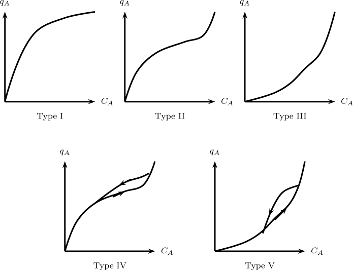
Figure 29.2 Five common types of adsorption isotherms according to Brunauer et al. (1938). Based on Hines and Maddox (1985).
Type I is the standard Langmuir isotherm and shows a monotonic approach to qmax; it applies for the case where the adsorption is restricted to a monolayer. Type II occurs when the monolayer adsorption occurs at low pressures and a multilayer condensation type of phenomena occurs at higher pressures. Type III is a case where the condensation type of phenomena is the dominant mechanism. Adsorbents showing this pattern are not useful in practice because the adsorbed concentration is low except at very high concentrations or pressures.
Types IV and V are systems showing a hysteresis phenomena, which is due to capillary condensation. These are capillary condensation versions of Type II and III, respectively.
29.3 Model for Batch Slurry Adsorber
Data from a batch adsorber provide a means of measuring equilibria and can also be used for small-scale processes for gas/liquid purification. Time versus liquid concentration profiles are calculated. In this section we show how mass balance equations can be combined with transport laws and an equilibrium model to predict the transients in this process.
29.3.1 Model Equations
Mass balance on the liquid phase in words is
Loss of solute in the liquid phase = Gain of mass in the solid phase
This can be written mathematically as
where is the average adsorbed concentration in the solid. CA is the concentration in the bulk liquid. The average concentration needs a transient diffusion model for the particle. This particle-level model is common to both the batch slurry adsorber discussed in this section and the fixed bed adsorber discussed in Section 29.4.
29.3.2 Particle-Level Model
The concentration in the particle varies as a function of position due to pore diffusion limitations. The local equilibrium is assumed for the adsorption process and hence the adsorbed concentration at any point in the solid, qA(r), is equal to KCAp(r). Here CAp is the concentration of A in the fluid phase in the pores at any location r.
Note: The notation K is used here for the linear adsorption relation as an abbreviation for the KA,linear in Equation 29.2. This should not be confused with the KA in the Langmuir model. Also qA will be abbreviated as q and CAp is abbreviated as Cp.
The average concentration in the pores (a spherical particle is assumed here) is given as
Using the local equilibrium relation, this can be written in terms of the pore level concentration Cp as:
The variation of Cp as a function of r can be modeled by the transient diffusion model:
The two terms on the left-hand side represent the mass capacity in the pores and the mass capacity on the solid. Usually K is large and the second term, the mass capacity over the solid, is much larger and hence in further discussion the first term is dropped. Also note that the surface diffusion (diffusion of adsorbed species along the surface) is ignored here and only the pore diffusion is included.
Since q = KCp (assuming a linear isotherm here) the PDE can also be written as
Equation 29.10 requires two boundary conditions and one initial condition. The center condition at r = 0 is the symmetry condition while the boundary condition at r = R depends on whether external mass transfer (liquid to solid) is important or not. Thus we can use the Dirichlet at the surface if the liquid to solid mass transfer is relatively fast compared to internal diffusion. This provides the following condition for the case of no external resistance:
If the external mass transport is included, a balance of flux at the solid surface leads to the following Robin condition:
The initial condition is taken as zero concentration, that is, a fresh adsorbent particle.
The solution of Equation 29.10 can be used in Equation 29.8 to get and , which in turn is needed in Equation 29.6. This is the exact procedure. It is useful to solve the particle model numerically since the analytical solution is cumbersome in spite of the fact that the PDE is linear. The solution can be done using orthogonal collocation, which appears to be the most efficient for this system. This method is discussed in Section 29.3.5. An approximate analytical solution is based on the linear driving force model, which is presented in the following section.
29.3.3 Linear Driving Force Model
The linear driving force model provides an approximation (LDF approximation). This was first introduced into the adsorption field by Glueckauf (1955). The concentration profile in the particle is assumed to a parabolic function in the derivation of this approximation. The concentration profiles and the LDF approximation to the internal profiles are shown in Figure 29.3.
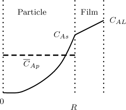
Figure 29.3 Concentration profile in a solid adsorbent and the external film at a given instant of time. The dotted line is the average concentration used in the LDF model.
The quadratic profile assumption can be used to derive an approximate lumped transfer coefficient for internal diffusion. Equivalently its reciprocal is the internal diffusional resistance. The external mass transfer leads to an additional drop in concentration from bulk to the surface. The overall resistance is then the sum of the external solid–liquid resistance and the internal diffusion resistance. The overall driving force is represented as . The rate of transfer is represented as a transfer coefficient, k0, times the driving force. Thus the uptake per particle volume is modeled as
The exchange resistance 1/k0 is modeled as the reciprocal of the sum of two resistances.
An approximate formula for this exchange coefficient is
The first term on the right-hand side is the resistance to solid–liquid mass transfer and the second term is resistance to internal diffusion.
The equivalent representation in terms of the resistance is presented in Figure 29.4. This figure captures the essence of the linear driving force model.

29.3.4 Calculation of the Slurry Transients
We now link the LDF model to the slurry mass balance model given by Equation 29.6. The average concentration in the adsorbent can be related to CAL by an overall balance from the start to any instantaneous time:
(Solute in liquid + solute in solid) at time t = Solute in liquid at time zero
Using this material balance, the following equation can be derived:
Here CAi is the initial concentration of the solute in the bulk liquid.
Using the above relation for in Equations 29.6 and 29.13, we can show that
An adsorption factor α is defined as
Using this factor Equation 29.16 is written as
Integration of Equation 29.16 provides the concentration profile in the liquid as a function of time. The resulting expression is
The final concentration in the liquid is obtained in the limit t tending to infinity:
This can also be verified by an overall mass balance from time 0 to ∞.
The final concentration depends only on α, which can be obtained by changing the volume of the liquid to that of the adsorbent, VL/VS. The measured value of the final composition is used to find the parameter α using Equation 29.19, which in turn provides the equilibrium constant, K. The assumption of linear equilibrium can also be tested by this set of experiments since K should be independent of the final concentration for a linear isotherm.
Note also that for each final concentration obtained by changing the VL/VS ratio, the corresponding adsorbed concentration is given by Equation 29.15:
This equation is independent of the type of isotherm since it is purely based on mass balance. Hence qA versus CA data can be obtained in a batch slurry experiment by merely changing the solid loading progressively and allowing each set to reach the steady state. The data can then be used to fit a suitable isotherm.
29.3.5 Simulation Using the Collocation Method
In order to simulate the batch slurry transients numerically one needs to discretize the spatial operator in Equation 29.10. One very useful tool is the orthogonal collocation method. We introduce this briefly here and show how the model can be reduced to a set of ordinary differential equations in time.
Equation 29.10 is first made dimensionless in distance by defining ξ = r/R, leading to
where K′ = K(1 – ∊p) is used as an abbreviated notation. Note that the time is not dimensionless here. The right-hand side is the Laplacian defined in dimensionless coordinates and can be approximated using the B matrix given in Section 18.6. This is applied at all the interior points leading to a set of equations for dCpi/dt:
Here N is the total number of collocation points and Cpi is the concentration of A in the pores at collocation point i.
The point N is the surface of the catalyst (r = R) and the concentration at this point, CpN , is assigned by using the the boundary condition given by Equation 29.12. Using the A matrix for the derivative, the collocation version of this boundary condition is
Here the parameter Bi is defined as = kmR/De. Rearranging this equation, the surface concentration is given as
Note that if Bi is large, the Dirichlet condition holds and CpN can be simply approximated as CAL. This is a case where the film mass transfer is rapid compared to internal diffusion.
An additional equation for dCAL/dt can be obtained from Equation 29.6. This needs an average adsorbed concentration, . The relation is used. The integral to calculate the average concentration in the pore, , is approximated using the w values, the quadrature weights, and therefore
Using this in Equation 29.6 and rearranging we get
where α is defined as VL/VSK′.
The initial value equations (Equations 29.22 and 29.26) can be readily integrated, for example, using ODE45. The time evolution of the concentration in the interior points in the pore and in the bulk liquid can then be calculated simultaneously. Further details are left as an exercise.
29.3.6 Additional Complexities
Other effects related to the model caused by additional complexities are discussed qualitatively here. Some useful references for further study are also provided.
Variable Diffusivity
This type of model arises when there is a significant concentration dependence on the intracrystalline diffusivity. An example is diffusion in molecular sieve zeolites. Numerical solutions for constant surface concentration have been presented by Garg and Ruthven (1973). A similar nonlinear dependence also arise for nonlinear adsorption isotherms due to the nonlinear dependency of q on Ci, for example, the Freundlich isotherm. Collocation methods are still suitable with the nonlinear dependent terms added to the B matrix. This presents an interesting case study for students. One consequence is that the adsorption and desorption curves are no longer mirror images of each other. For large concentration values, the adsorption front moves faster than desorption and vice versa.
Bidispered Particles
Many commonly used adsorbents contain both macropores and micropores; these have a grain or particle-pellet structure similar to that discussed in Section 19.3. In this case the macropores provide the transport pathways while the major adsorption takes place in the micropores. Detailed modeling and a solution were presented by Gray and Do (1991) and Liu and Bhatia (2001) and for more details these sources are useful.
29.4 Fixed Bed Adsorption
Fixed bed adsorption columns are commonly used in industrial practice. In this mode of operation the feed containing a solute to be removed is continuously introduced to the system. The column operates in a transient mode and the effluent concentration of the solute varies with time. This concentration is monitored and the operation is stopped when the effluent concentration increases above a threshold value. The adsorbent bed is then regenerated and the operation repeated. Usually two beds are used in tandem, one in adsorption mode and the second in regeneration mode so that uninterrupted continuous operation can be achieved. This section provides an analysis of the transient concentration profiles in fixed bed adsorption and indicates some design considerations.
The model is similar to the tracer response curve in a packed bed studied in Chapter 14. Modeling can be done on many levels of progressive complexity and the approach is discussed in the following.
Models where the concentration profiles in the solid are not solved explicitly are called pseudo-homogeneous models. If the profiles in the solid are also included the model is a called heterogeneous model. The pseudo-homogeneous type of model can again be developed at various levels of detail.
The first category of model is based on local equilibrium and provides an approximate estimate of the column size needed and also the effect of the adsorption isotherm on the outlet concentration. Here no mass transfer resistances are considered nor is the effect of axial dispersion.
A second level of model keeps the local equilibrium assumption but introduces the axial dispersion effect.
The third level includes the mass transfer resistances in addition to dispersion. But the particle-scale model is not solved in detail and instead lumped into an overall mass transfer coefficient based on the LDF concept.
Models where the solid concentration profile is also included and the gas and solid are treated as separate phases are called heterogeneous models. The gas phase is modeled using dispersion and the solid phase is modeled using a transient diffusion-adsorption model; the two are coupled and solved simultaneously.
29.4.1 Equilibrium Model
Plug flow of gas is assumed and local equilibrium between gas and solid is assumed at each point in the adsorber. Transport effects are not included. The gas balance is done by writing the mass balance:
in – out = accumulation
In = uGA(CA)x where uG is the superficial velocity of the gas. Similarly, out = uGA(CA)x+Δx.
The accumulation is the time derivative of moles of A in the system. Moles of A are present in the gas phase in the void space plus that adsorbed on the solids. The adsorbed concentration is in equilibrium with the gas concentration. Hence the adsorbed concentration is equal to KACA for linear adsorption. Combining the two, the following expression is obtained for the moles of A in the differential volume:
Moles of A = [∊B + KA(1 – ∊B)] CAAΔx
Here ∊B is the bed voidage, that is, the fraction of the bed that is not occupied by the solid.
Putting all these together into the gas phase balance, we can derive the following differential equation for the concentration variation of A in the system:
A wave speed ws can be defined as
Using this Equation 29.27 can be expressed in a simpler form as
This is the simplest PDE of the hyperbolic type. The equation requires an inlet condition CAi(0, t) (which can be any a specified function of time) and an initial condition (taken as zero here). The solution is simply a time delay:
Here H is the Heaviside step function.
The inlet value simply moves along the bed with the wave velocity. The inlet response therefore appears at position x after an elapse of time of L/ws for a step input.
The time constant for a plug flow, also called the retention time (which is also the first moment of the system for a pulse input) is given by
The second moment can be shown to be equal to zero and therefore there is no spread or dispersion. A pulse introduced at the inlet will appear at the exit intact after the elapse of this retention time. Similarly a square wave input at the inlet will appear at the exit as a square wave after this time. A step input will appear as a step input at the exit after the elapse of the retention time.
The exit response is shown schematically in Figure 29.5. (Note that the ∊B term in Equation 29.31 is normally dropped as done in this figure.)

Figure 29.5 Exit response to a pulse injection in an adsorption column modeled as plug flow with an equilibrium model.
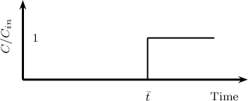
The exit response to a step input is shown in Figure 29.6. For a continuous flow of solute with the inlet gas, no solute appears in the exit for time less than the retention time. After this time, the exit concentration is equal to the inlet concentration. Hence for a given length of the bed the maximum time of operation is equal to the retention time.
29.4.2 Axial Dispersion Effects
In reality the response is not a sharp jump as depicted in the previous figure but is instead broadened due to axial dispersion effects. Another factor that can cause spreading is the internal diffusion and in some cases the solid–liquid film mass transfer. Each of these contribute to the variance of the pulse response or to the spread of a step response. The characteristic exit then shows a spread around the retention time. The resulting curve is called the breakthrough curve and is sketched in Figure 29.7. Note that a part of the solute appears earlier than the retention time and some appears after the retention time. If a certain cutoff purity is required at the exit, the operating time has to be reduced. This results in a part of the bed not being utilized. If the exit concentration has to be less than, say, Cb then the operating time should be tbthe corresponding time on the breakthrough curve.

Figure 29.7 Breakthrough curve with exit concentration as a function of time. Data from Hines and Maddox (1994).
The steepness of the breakthrough curve shows how much of the bed is underutilized. If it is very steep a large part of the bed is utilized, approaching an ideal case. Thus prediction of the shape of the breakthrough curve is quite important. It is also useful to know what effects the bed length, bed diameter, and particle diameter have on the shape of the breakthrough curve. The mass transfer models are useful to do these calculations.
The spread due to dispersion is modeled by adding an additional contribution to axial dispersion, but other assumptions in the ideal model are retained. Thus film diffusion and internal diffusion are not accounted for and a local equilibrium is assumed at any location in the adsorber. This, for example, could apply for small particles where the mass transfer coefficients are large and the internal diffusion resistance is also small.
The gas balance now reads
where the first term on the right-hand side reflects the spread due to axial dispersion. The model now needs one initial condition and two boundary conditions. This is similar to the dispersion model studied in Section 14.3. The time constant is simply adjusted to account for the accumulation in the solid. The response curve would look similar to that plotted in Figure 14.2.
The dispersion coefficient is an important parameter in quantifying the pulse spread. Correlations to calculate these were reviewed in Section 14.6 and are useful to simulate adsorption and chromatographic columns.
29.4.3 Heterogeneous Model
In this model the gas and solid are modeled separately with the solid–liquid mass transfer connecting the two models. The model equations are stated below. See also the discussion in Section 14.5 where the variance of the tracer curve is shown for a packed bed. It may be useful to review this section at this point.
The gas balance equation is now modeled with the accumulation in the particle added as an additional term. The assumption is no longer used:
where is the average concentration in the solid:
The variation of qA as a function of r can be modeled by the transient diffusion model. This part of the model is given in Section 29.3.2.
The solution of this model needs a coupled computational scheme. At each location x in the bed, the particle model has to be solved to provide the information. This provides the required coupling for the gas phase balance. A number of numerical methods can be used. Collocation methods are again suitable but need some additional refinements. Since there are two spatial variables, one in the bed x and the second internal to the particle r, two separate collocation discretizations are needed. The method is sometimes called double collocation. Sampath et al. (1975) provide details of this method. Although this paper is for a reacting solid problem it has the same mathematical structure as the transient adsorption simulation model.
29.4.4 Klinkenberg Equation
A useful approximate analytical solution to calculate the breakthrough curve was developed by Klinkenberg (1962). Here axial dispersion is not included but mass transfer effects are. But the particle model is not solved and the LDF approximation is used to account for mass transfer and internal diffusion. The concentration profile is given by the following equation as a function of dimensionless distance and time:
Here ξ is the dimensionless axial distance, defined as
and τ is dimensionless time corrected for the motion of the fluid, defined as
Here k0 is given by the LDF model (Equation 29.14).
29.4.5 Scale-Up Aspects
Often data from small-scale columns needed to measure adsorption capacity; the data are used to predict the performance of large-scale columns. Crittenden and Thomas (1998) suggested the following scale-down rules:
where ts is the time for estimated breakthrough in a small-scale column and tL is the value for the large-scale column. dp is the particle diameter used.
The exponent of the particle diameter α has a value of 0 for a constant diffusion coefficient and is equal to 1 for diffusivity proportional to concentration. The latter value is representative if surface diffusion is the dominant pore transport mechanism. Spread by internal diffusion is the main controlling mechanism implied in this scale-up rule. Since the time constant for the constant diffusivity is proportional to the square of the diameter, the exponent is two for the constant diffusivity case.
The matching of the Reynolds number is used to determine the operating velocity in the small columns. Hence
Particle to column diameter should be chosen as 20 or more to avoid channeling near the walls.
29.5 Chromatography
Chromatography is a generic term to denote separation of multicomponent mixtures by using the difference in adsorptivity. The principle behind chromatography is similar to adsorption. Both involve contacting a multicomponent fluid mixture with a solid. The only difference is that the solute is injected as a pulse and usually has many components. An inert carrier gas is used as a base component and this provides the motion of the pulse in the bed. The process is also known as elution chromatography since the pulse is eluted by the carrier stream. Depending on the relative magnitude of the adsorption constants, two components appear at the exit at different times and chromatographic separation is achieved. Chromatography is mainly used as an analytic tool. Large-scale chromatography can be used for separation of liquid mixtures; the separation of xylene isomers is an example.
We first look at the process assuming plug flow and then correct the model for the effect of axial dispersion. The pulse of A will appear intact after the elapse of retention time if there are no factors that cause the broadening of the pulse. The retention time for A is given as
Note that the mean retention time depends on the adsorption constant, as observed from the above equation. If the two solutes have different mean retention times, they appear in the exit stream at different times, causing a separation. This is the principle of chromatography. If the column is modeled as an ideal system, the two components will appear as two sharp peaks at the corresponding mean retention time. In reality, there are dispersion effects, which cause a spread; this is referred to as pulse broadening. An illustrative response curve is shown in Figure 29.8.
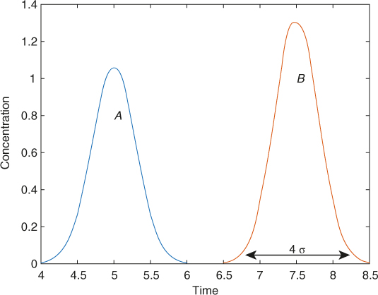
Figure 29.8 Typical response for a binary mixture; the peak spread width Δt corresponds to four times the standard deviation. and . Time is arbitrary units for illustration purposes only.
If the injected sample is small, the pulse becomes Gaussian and the concentration distribution can be modeled as a Gaussian distribution around the mean:
The variance depends on the extent of axial dispersion, solid–liquid mass transfer, and the internal diffusion. Each term contributes in an additive manner to the variance. Equation 14.45 can be used to estimate the contribution of the above three factors to the variance. The spread around the mean retention time is about 4σ, as shown in Figure 29.8 for a Gaussian distribution.
The area under the curve is a measure of the amount of that component. Overlapping peaks are often noticed. This depends on the σ parameter, which causes the spread. If and are somewhat close and simultaneously if σ is also high, then overlap will result. Any factor that decreases σ will help in reducing the overlap. For example, increasing the column length can be helpful. Change in temperature, temperature programing, change in carrier gas composition, or change in column material are other tools which can be used to increase the resolution between adjacent peaks.
Summary
Adsorption is a process where a solute is transferred from a fluid phase to the surface of a solid and retained there. It is generally used for purification of waste streams. Some large-scale processes are also in practice, for example, separation of air into nitrogen and oxygen, and separation of isomers such as xylene.
Adsorption isotherms show the equilibrium relation between the gas concentration and the adsorbed concentration. For low concentrations a linear relation is used while for high concentrations, the Langmuir or Freundlich isotherm is commonly used.
The BET isotherm accounts for multiple layers over the solid and is generally of five types: monolayer adsorption, monolayer adsorption followed by multilayer condensation, multilayer condensation, and capillary condensation with hysteresis of two types (convex upward and convex downward).
Batch slurry adsorption is used in small-scale systems and also as an experimental tool to determine adsorption rate and equilibrium. The process requires two transport steps: film mass transfer and internal diffusion in the pores. Particle-level transient diffusion models can be set up and coupled to a macroscopic balance for the liquid in order to track the concentration changes in the liquid with time. The coupled model can be solved by the orthogonal collocation method.
The LDF model provides a simpler approach for the particle-scale model. The diffusion equation for a concentration profile within the particle is not used and lumped into an internal transport coefficient. An overall mass transfer coefficient can be defined on this basis and combined with the solute mass balance in the bulk liquid. Analytical solutions result for the linear adsorption model.
In an ideal fixed bed operation, the fluid is assumed to be in equilibrium with the local fluid concentration. No other effects are included. The results show that a sharp concentration front develops in the bed. This front moves with a velocity known as the wave velocity, which is given by Equation 29.28. The corresponding time constant is called the retention time. The solute breakthrough is achieved after the retention time and the bed can be operated up to this time.
When mass transfer effects are included, the ideal response is not seen and instead an S-shaped curve is observed for the exit concentration. This curve is called the breakthrough curve. The time of operation is reduced due to the S-shaped nature and a portion of the bed will remain unused.
The Klinkenberg model is a useful model to predict the breakthrough curve. The model provides useful information to scale up laboratory data to large-sized commercial units. The model does not include axial dispersion and also assumes a linear adsorption isotherm. Also it uses the LDF approximation for the particle scale transport.
Chromatography is a generic term to denote separation of multicomponent mixtures by using the difference in adsorptivity. The principle behind chromatography is similar to adsorption. Both involve contacting a multicomponent fluid mixture with a solid. The only difference is that the solute is injected as a pulse and usually has many components.
Review Questions
29.1 What is the mechanistic basis for the Langmuir model?
29.2 How should the experimental data of q versus CA be plotted in order to test the Langmuir model?
29.3 State the Freundlich isotherm and also the units of the equilibrium constant used in the model.
29.4 How should the experimental data of q versus CA be plotted in order to test the Freundlich model?
29.5 If a plot of 1/q versus 1/CA is linear, what do the slope and intercept represent?
29.6 If a log-log plot of q versus CA is linear, what do the slope and intercept represent?
29.7 What can cause hysteresis behavior in an adsorption isotherm, that is, are the q versus CA plots different for adsorption compared to that for desorption?
29.8 What is the LDF approximation?
29.9 What is the assumption used to derive the LDF approximation?
29.10 What are the differences between the pseudo-homogeneous model and heterogeneous model for packed columns?
29.11 What is the ideal pulse velocity in an adsorption or chromatographic column?
29.12 What is the breakthrough curve?
29.13 What principle is used in chromatographic separation?
29.14 What factors cause pulse broadening in a chromatographic column?
Problems
29.1 Fitting an isotherm to data. The following data were obtained for adsorption of pure methane on activated carbon by Ritter and Yang (1991):
q, STP cm3/gm |
40 |
165 |
350 |
545 |
760 |
910 |
970 |
p, atm |
45.5 |
91.5 |
113 |
121 |
125 |
126 |
126 |
Fit a suitable isotherm model for the this data. Deterimine which isotherm (Langmuir or Freundlich) provides a better fit to the data.
29.2 Batch adsorber calculations. An aqueous solution of phenol with a concentration of 0.01 mol/L is treated with activated carbon in a batch adsorber. An adsorbent loading of 10 g/L is used. The equilibrium constant K has a value of 100. The external mass transfer coefficient is 5 × 10⁻⁵ m/s. The internal diffusion coefficient is 2 × 10⁻⁹ m2/s and the particle size used is 1.5 mm diameter. Find the α parameter and use this to find the final concentration of phenol in the liquid. Find the k0 parameter and use this to track the concentration versus time profile of phenol in the liquid.
29.3 Laplace transform method. Obtain the solution to Equation 29.29 in the Laplace domain. Find the first and second moments and verify the expression for the time constant is given in Equation 29.31 and also that the variance is zero. Look up books that provide a table of inverse transforms and verify the time domain solution given in the text.
29.4 Ideal adsorption model. An aqueous solution of 3 g/cm3 each of glucose and fructose is fed into an adsorption column packed with an ion exchange resin. The adsorption isotherm is modeled as a linear equation q = KCA with K = 0.26 for glucose and K = 0.40 for fructose. The units are g per 100 cm3. The superficial velocity is 0.031 cm/s and the bed void fraction is 0.4. If the feed is introduced as a sharp pulse in a column of length 200 cm, determine the time when the two solutes appear at the exit. If a square wave feed pulse lasting 500 seconds is introduced, sketch the exit concentration of both the solutes. Assume the pulse travels as a wavefront with the wave velocity given by Equation 29.28.
29.5 Wave speed for nonlinear equilibrium. A wave speed ws was shown to be given by Equation 29.28 for a linear adsorption isotherm. Show that for a nonlinear isotherm the wave speed can be calculated as
29.6 Klinkenberg model for breakthrough. Air at 25 °C and 1 atm containing 0.9% benzene is fed to an adsorption tower that is 30 cm in diameter and 2 m long. The air flow rate is 5 kg/min. The bed is packed with silica gel with an effective diameter of 2.6 mm. The bed void fraction is 0.5. The isotherm is linear with K equal to 5.2. The mass transfer coefficient k0 was found from separate experiments to have a value of 0.2 min–1. Calculate the retention time. Use the Klinkenberg model and plot the breakthrough curve. Find the time at which 5% benzene appears in the exit. Find the fraction of the bed that is not utilized. Repeat the calculation if the bed were 8 m long. Determine by what factor the pressure drop would increase. Note that the cost of pumping has to be balanced with the need for more frequent regeneration.
29.7 Packed bed: size specifications. A packed column is used to separate a solute from an air stream of 1 L/min flow. A superficial velocity of 4 cm/s is suggested and the column will operate for 4 hours before regeneration. The equilibrium constant is 500. The exit stream should contain no more than 5% of the incoming solute. The particle size is 3 mm and the bed void fraction 0.4. The diffusion coefficient of the solute in air is 0.16 cm2/s. Calculate the solid–liquid mass transfer coefficient and the k0 parameter. Find the column height needed. Find the pressure drop in the column. Examine the sensitivity of your results by changing the superficial velocity and the suggested operation time.
29.8 Scale-up of a packed adsorber. A small-scale unit is operating with a particle radius of 0.1 mm at a velocity of 25 m/hour and the breakthrough was observed after 24 sec. Based on this what should be operating velocity if a pilot scale adsorber will operate at 5 m/hour? What would be breakthrough time in this column?
29.9 Chromatographic separation. Consider separation of two components with the following properties: KA = 1; KB = 2; DA = 2 × 10⁻⁴ m2/s; DB = 8 × 10⁻⁴ m2/s. The eluting fluid has a flow rate of 1 cm3/min and the column of diameter of 5 mm. The length of the column is 2 m. The particle size is 0.5 mm.
Find σ and test if there is an overlapping of the peaks. Assume that the spread is due to internal diffusion only.
Sketch and plot the exit concentrations of the two solutes as a function of time.