Chapter 5. Equations of Mass Transfer

Search in book...
Toggle Font Controls
Create new playlist

Name your new playlist

Playlist description (optional)
Sign In

Email address

Password

Forgot Password?

or

Continue with Facebook

Continue with Google
Sign Up

Full Name

Email address

Confirm Email Address

Password

or

Continue with Facebook

Continue with Google

Chapter 5. Equations of Mass Transfer

Learning Objectives

After completing this chapter, you will be able to:

Derive differential equations for mass transfer in Cartesian coordinates in flux form.
Express these relationships in vector form so that they can be used for any coordinate system.
Define the mixture velocity and the diffusion flux.
Examine some properties of the diffusion flux.
State some forms of Fick’s law for binary systems depending on the frame of reference used.
Derive the differential equation for the concentration field by combining the equation in the flux form with Fick’s law.
State the boundary conditions for many standard cases.
Show how averaging of differential models leads to mesoscopic and macroscopic models, and describe the relationship between these models.
Show how the differential models for two flowing phases arise by local volume averaging of the individual continuity equation.

Chapter 1 examined the basic philosophy behind mathematical modeling of mass transport processes, and Chapter 2 demonstrated the methodology with a few examples on a problem to problem basis. We examined how the mass conservation principle combined with a simple Fick’s law as a constitutive equation can be used to set up differential models for some common problems posed in simple 1-D coordinates. Chapters 3 and 4 provided some examples of macroscopic and mesoscopic models, again on a problem to problem basis.

The goal of this chapter is to explore these topics in a more formal setting and derive general differential equations for concentration distribution. We first apply the conservation law to derive the equations in flux form. The diffusion flux must be closed at this point to get the equations in concentration form.

In dealing with mass transfer problems, an important concept is the system average velocity and the frame of reference used to define the diffusion flux of various species. The system average velocity can be defined in a number of ways, and the diffusion flux can be correspondingly defined in a number of ways. Thus, even the simple Fick’s law for binary diffusion takes various forms depending on which frame of reference is used. These subtleties can be a source of confusion for the uninitiated. To clarify them, these concepts are defined in Section 5.2.

The next step in completing the differential models is to combine the constitutive model (usually a Fick’s law model or some version of it) for the flux with the mass conservation equation. This then leads to a differential equation of mass transfer in concentration form. This equation represents the starting point for the analysis and modeling of a range of mass transport problems and has wide applications in many fields. Commonly used boundary conditions for various cases are then formulated, which completes the model formulation.

A volume average of the differential model over a larger control volume or the whole unit provides the macroscopic model for mass transfer. The necessary equations are formally derived starting from the differential models. Mesoscopic models can also be derived in a similar manner. Deriving these by averaging provides the link between the two levels of models and shows the interpretation of the various terms as integrals of pointwise values of the differential model. Closure assumptions needed in these models are clearly identified in the process.

Systems with two or more phases can be treated in the same manner, by starting with local volume averaging to obtain the differential equations for each of these phases. The interfacial transfer term arises naturally as a consequence of local volume averaging. Additional cross-sectional averaging leads to two-phase mesoscopic models. Similarly, averaging over a larger volume of local volume averaged models leads to two-phase macroscopic models. This systematic way of deriving the equations assigns the meaning to various terms and identifies the needed closure terms.

5.1 Flux Form

The equations for mass transfer can be derived in either mass units or mole units. In the combined flux form, these equations can be easily interconverted using the species molecular weight (mass = moles × the species molecular weight). We first show the equations on mole basis.

5.1.1 Mole Basis

Consider the control volume shown in Figure 1.9 in the shape of a box. This box has six control surfaces. We take them pairs and evaluate the net mole efflux from the control surfaces.

The faces at x and x + Δx are taken as a first pair. The moles of A leaving the face x + Δx per unit time is flux at the point times area, and is equal to N_Ax evaluated at x + x times the area of the plane, Δy Δz.

Moles of A leaving in x-direction/time = N_Ax(x + Δx) Δy Δz

Using Taylor series, we can approximate

N_{A x} (x + Δ x) = N_{A x} (x) + \frac{\partial}{\partial x} (N_{A x}) Δ x

$N_{A x} (x + Δ x) = N_{A x} (x) + \frac{\partial}{\partial x} (N_{A x}) Δ x$

Here, the derivative term on the right side is evaluated at x. Hence we have

Moles leaving in x -direction = N_{A, x} (x) Δ y Δ z + \frac{\partial}{\partial x} (N_{A, x}) Δ x Δ y Δ z

$Moles leaving in x -direction = N_{A, x} (x) Δ y Δ z + \frac{\partial}{\partial x} (N_{A, x}) Δ x Δ y Δ z$

The first term on the right side is moles of A entering the plane at x.

The net mole efflux (leaving minus entering) from the two planes at x and x + Δx is

Net mole efflux' from x -faces = \frac{\partial}{\partial x} (N_{A x}) Δ x Δ y Δ z

$Net mole efflux' from x -faces = \frac{\partial}{\partial x} (N_{A x}) Δ x Δ y Δ z$

The net mole efflux per unit control volume is therefore is obtained by dividing by the size of the control volume:

Net mole efflux per unit volume; x -faces only = \frac{\partial}{\partial x} (N_{A x})

$Net mole efflux per unit volume; x -faces only = \frac{\partial}{\partial x} (N_{A x})$

Similar expressions can be obtained for the y- and z-planes. Thus the net mole efflux per unit volume is equal to

Net mole efflux per unit volume; from all six faces = \frac{\partial}{\partial x} (N_{A x}) + \frac{\partial}{\partial y} (N_{A y}) + \frac{\partial}{\partial z} (N_{A z})

$Net mole efflux per unit volume; from all six faces = \frac{\partial}{\partial x} (N_{A x}) + \frac{\partial}{\partial y} (N_{A y}) + \frac{\partial}{\partial z} (N_{A z})$

Students proficient in vector calculus will quickly recognize this as the divergence of the flux vector N A in Cartesian coordinates. The previous expression can be written compactly using vector notation as follows:

\begin{matrix} Mole efflux per unit volume = \nabla \cdot N_{A} & (5.1) \end{matrix}

$\begin{matrix} Mole efflux per unit volume = \nabla \cdot N_{A} & (5.1) \end{matrix}$

Although derived using Cartesian control volume, this expression in vector form is general and is applicable to any other coordinate system (e.g., cylindrical, spherical). The appropriate form of the divergence expression is used for a given coordinate system to get the detailed expression for the mole efflux in that coordinate system.

The accumulation of A in the control volume is ∂C_A∂t per unit control volume.

The mole rate of production of A is denoted as R_A per unit control volume.

The conservation statement is

in – out + net generation = accumulation

Alternatively, noting that

out – in = net efflux

we have

–net efflux + net generation = accumulation

Combining the derived forms for each of the terms, we get the the vector form of the species mass balance equation:

\begin{matrix} \begin{matrix} - ▽ \cdot N_{A} + R_{A} = \frac{\partial C_{A}}{\partial t} \end{matrix} & (5.2) \end{matrix}

$\begin{matrix} \begin{matrix} - ▽ \cdot N_{A} + R_{A} = \frac{\partial C_{A}}{\partial t} \end{matrix} & (5.2) \end{matrix}$

This vector form is applicable to any coordinate system with the divergence defined appropriately for that coordinate system. The form of the divergence in three common coordinate systems is shown next for ease of reference.

Divergence operator in three common coordinate systems

Cartesian:

\nabla \cdot N_{A} = \frac{\partial}{\partial x} (N_{A x}) + \frac{\partial}{\partial y} (N_{A y}) + \frac{\partial}{\partial z} (N_{A z})

$\nabla \cdot N_{A} = \frac{\partial}{\partial x} (N_{A x}) + \frac{\partial}{\partial y} (N_{A y}) + \frac{\partial}{\partial z} (N_{A z})$

Cylindrical:

\nabla \cdot N_{A} = \frac{1}{r} \frac{\partial}{\partial r} (r N_{A r}) + \frac{1}{r} \frac{\partial N_{A θ}}{\partial θ} + \frac{\partial N_{A z}}{\partial z}

$\nabla \cdot N_{A} = \frac{1}{r} \frac{\partial}{\partial r} (r N_{A r}) + \frac{1}{r} \frac{\partial N_{A θ}}{\partial θ} + \frac{\partial N_{A z}}{\partial z}$

Spherical:

\nabla \cdot N_{A} = \frac{1}{r^{2}} \frac{\partial}{\partial r} (r^{2} N_{A r}) + \frac{1}{r \sin θ} \frac{\partial}{\partial θ} (N_{A θ} \sin θ) + \frac{1}{r \sin θ} \frac{\partial N_{A φ}}{\partial φ}

$\nabla \cdot N_{A} = \frac{1}{r^{2}} \frac{\partial}{\partial r} (r^{2} N_{A r}) + \frac{1}{r \sin θ} \frac{\partial}{\partial θ} (N_{A θ} \sin θ) + \frac{1}{r \sin θ} \frac{\partial N_{A φ}}{\partial φ}$

5.1.2 Mass Basis

The equations can be also based on mass units using the following conversion: N_A = n_A/M_A. For example, Equation 5.2 can be expressed in mass units as:

\begin{matrix} \begin{matrix} - \nabla \cdot n_{A} + r_{A} = \frac{\partial ρ_{A}}{\partial t} \end{matrix} & (5.3) \end{matrix}

$\begin{matrix} \begin{matrix} - \nabla \cdot n_{A} + r_{A} = \frac{\partial ρ_{A}}{\partial t} \end{matrix} & (5.3) \end{matrix}$

where r_A is the mass rate of production (kilograms produced per unit time per unit volume), which is in turn equal to R_AM_A.

Equations 5.2 and 5.3 are both in flux form since the combined flux vector (either mass units or molar units) appears as a term the equations. To proceed further, we need to split the combined flux into a convection flux and a diffusion flux, and then incorporate a suitable expression for diffusion flux (the constitutive model). This will provide the equation in the concentration form rather than in the flux form, which is appropriate since we want to solve for the primary field variable, the species concentration.

One problem is that diffusion flux is not uniquely defined; that is, it can be defined in many ways. Our goal now is to define this component more precisely compared to the simple definition used in Chapters 1 and 2. Specifically, we need a definition of the frame of reference (mixture average velocity) because diffusion flux is defined assuming that the system has no net velocity—that is, the flux is assumed to be from diffusion only. Diffusion flux must therefore be defined with reference to a coordinate system with zero velocity.

5.2 Frame of Reference

One confusing aspect of a multicomponent mixture is that there are many ways to define the average velocity of a mixture, and correspondingly there are many definitions of diffusive flux. In general we can write the following expression in mole units:

J_{A}^{ref} = N_{A} (fixed) - C_{A} υ^{ref}

$J_{A}^{ref} = N_{A} (fixed) - C_{A} υ^{ref}$

Alternatively, we can write the expression in mass units by multiplying by M_A:

j_{A}^{ref} = n_{A} (fixed) - ρ A υ^{ref}

$j_{A}^{ref} = n_{A} (fixed) - ρ A υ^{ref}$

The diffusion flux (in either units) is therefore obtained by subtracting the convective part from the combined flux (which is fixed). The convective part, in turn, uses a reference velocity (the mixture velocity, υ_ref), which can be defined in many ways. The combined flux N A or n_A is fixed at a given point; in contrast, υ and correspondingly J_A or j_A are not, but rather depend on how you define υ.

Two common ways of defining the reference velocity are the mole fraction weighted average velocity and mass fraction weighted average velocity. These concepts are introduced now, and Fick’s law for binary diffusion is revisited in this setting.

5.2.1 Mass Fraction Averaged Velocity

We start off by assigning a velocity to each of the diffusing species and then averaging these with a weighting factor to define a mixture velocity.

Species Velocity

Let n_A be the flux vector in mass units at a given point. Correspondingly, a velocity for species A, υ_A, can be defined at this point, which is related to mass flux vector by the mass concentration of A:

ρ_Aυ_A = n_A

Similarly, the velocity of B can be defined (as well other components in the system):

ρ_Bυ_B = n_B

Mixture Average Velocity

The mixture velocity υ is defined as a weighted average of the species velocities. Various definitions arise depending on which weighting factor is used to define this average. Here, we will use the mass fraction as the weighting factor. Thus the mixture velocity can be defined as follows for a binary mixture:

\begin{matrix} υ^{(m)} = ω_{A} υ_{A} + ω_{B} υ_{B} & (5.4) \end{matrix}

$\begin{matrix} υ^{(m)} = ω_{A} υ_{A} + ω_{B} υ_{B} & (5.4) \end{matrix}$

More generally, it can be defined as follows for a multicomponent mixture:

\begin{matrix} υ^{(m)} = \sum w_{i} υ_{i} = (\sum ρ_{i} υ_{i}) / ρ & (5.5) \end{matrix}

$\begin{matrix} υ^{(m)} = \sum w_{i} υ_{i} = (\sum ρ_{i} υ_{i}) / ρ & (5.5) \end{matrix}$

Here the summation is over all the species present in the system (i = 1 to ns). This mixture velocity is also referred to as mass-centric velocity.

A flux with respect to a moving frame can now be defined. Let the moving frame have velocity of υ^(m) (the mass averaged velocity). We will define relative velocity and then use this definition to define the fluxes. Let

j_{A}^{(m)} = ρ_{A} (υ_{A} - υ^{(m)})

$j_{A}^{(m)} = ρ_{A} (υ_{A} - υ^{(m)})$

represent the mass flux vector seen by an observer who is moving with the mixture velocity υ^(m). This mass flux can be attributed to only diffusion since the system (relative) velocity is zero in the case of a moving observer. Hence $j_{A}^{(m)}$ $j_{A}^{(m)}$ is one way of defining the diffusion flux. (The second way of defining the diffusion flux uses the mole centric velocity discussed in 5.2.2.) The flux defined in these two frames are shown schematically in Figure 5.1.

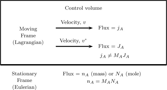
Diagrammatic illustration of the notions of combined flux and diffusion flux.

Figure 5.1 Schematic of the definitions of combined flux (frame of stationary observer) and diffusion flux (frame of moving observer).

Note: In the following section and most places in the text, $j_{A}^{(m)}$ $j_{A}^{(m)}$ will be abbreviated as j_A and υ^(m) will be denoted as υ.

The flux in a stationary frame is related to the flux in a moving frame as follows:

\begin{matrix} n_{A} = ρ_{A} (υ_{A} - υ) + ρ_{A} υ = j_{A} + ρ_{A} υ & (5.6) \end{matrix}

$\begin{matrix} n_{A} = ρ_{A} (υ_{A} - υ) + ρ_{A} υ = j_{A} + ρ_{A} υ & (5.6) \end{matrix}$

\begin{matrix} \begin{matrix} \begin{matrix} n_{A} \end{matrix} = j_{A} + ρ A υ \end{matrix} & (5.7) \end{matrix}

$\begin{matrix} \begin{matrix} \begin{matrix} n_{A} \end{matrix} = j_{A} + ρ A υ \end{matrix} & (5.7) \end{matrix}$

The two fluxes n_A and j_A and the corresponding observers are shown in Figure 5.1. Note that the left side of Equation 5.7 is the combined flux, the first term on the right side is the diffusion flux, and the second term on the right side is the convection flux.

It follows that ρ_Aυ = ω_Aρv and ρυ = n_t, the total flux (mass units). Hence ρ_Aυ = ω_An_t and the previous expression for the combined flux can be written as

\begin{matrix} n_{A} = j_{A^{+ ω} A} n_{t} & (5.8) \end{matrix}

$\begin{matrix} n_{A} = j_{A^{+ ω} A} n_{t} & (5.8) \end{matrix}$

The total flux n_t is equal to n_A + n_B in a binary mixture.

Fick’s Law: Version for j_A

For a binary system, the following constitutive model is applicable with the flux j_A seen to be proportional to the mass fraction gradient:

\begin{matrix} j_{A} = - ρ D_{A B} \nabla ω_{A} & (5.9) \end{matrix}

$\begin{matrix} j_{A} = - ρ D_{A B} \nabla ω_{A} & (5.9) \end{matrix}$

In this version of Fick’s law, D_AB is the diffusivity of A in the binary mixture of A and B. Note that we use D_AB for D_A. It turns out that for a binary system, D_A = D_B; this diffusivity is denoted as D_AB, meaning the binary pair diffusivity of A-B pair. This interpretation is proved in a later section.

5.2.2 Mole Fraction Averaged Velocity

The species velocity can also be defined using mole units. Thus, if N_A is the flux vector in mole units and C_A is the concentration, the following definition applies for the species velocity. This definition for v_A is the same as that obtained from using mass units:

\begin{matrix} N_{A} = C_{A} υ_{A} & (5.10) \end{matrix}

$\begin{matrix} N_{A} = C_{A} υ_{A} & (5.10) \end{matrix}$

Let υ* be the average (mole fraction weighted) velocity of the system defined as follows:

\begin{matrix} υ^{*} = \sum_{i = 1}^{n s} y_{i} υ_{i} & (5.11) \end{matrix}

$\begin{matrix} υ^{*} = \sum_{i = 1}^{n s} y_{i} υ_{i} & (5.11) \end{matrix}$

where y_i is the mole fraction of species i. This mole-centric velocity differs from the mass-centric velocity υ^(m) (more simply abbreviated as υ, as indicated earlier). In general, mass fraction is not equal to mole fraction, so the two velocities are different.

For an observer who moves with a system with a velocity of υ*, the flux observed will be

\begin{matrix} J_{A}^{*} = C_{A} (υ_{A} - υ^{*}) & (5.12) \end{matrix}

$\begin{matrix} J_{A}^{*} = C_{A} (υ_{A} - υ^{*}) & (5.12) \end{matrix}$

Rearranging Equation 5.12, we have

\begin{matrix} C_{A} υ_{A} = J_{A}^{*} + C_{A} υ^{*} & (5.13) \end{matrix}

$\begin{matrix} C_{A} υ_{A} = J_{A}^{*} + C_{A} υ^{*} & (5.13) \end{matrix}$

We therefore find the following relation between the (molar) flux in a stationary frame and in a moving frame:

\begin{matrix} N_{A} = J_{A}^{*} + C_{A} υ^{*} & (5.14) \end{matrix}

$\begin{matrix} N_{A} = J_{A}^{*} + C_{A} υ^{*} & (5.14) \end{matrix}$

where the first term on the right side is referred to as the diffusive flux and the second term is the flux arising out of the net fluid motion (the convective flux). The two fluxes N_A and J_A and the corresponding observers are shown in Figure 5.1.

Equation 5.14 can also be expressed in terms of the mole fraction:

\begin{matrix} \begin{matrix} N_{A} = J_{A}^{*} + y_{A} N_{t} \end{matrix} & (5.15) \end{matrix}

$\begin{matrix} \begin{matrix} N_{A} = J_{A}^{*} + y_{A} N_{t} \end{matrix} & (5.15) \end{matrix}$

where N_t is the total molar flux (stationary observer). This follows from Equation 5.14 since υ* = N_t/C.

Note: The star superscript on J will be dropped and we will denote J*_A as J_A in further discussions.

Fick’s Law: Mole Fraction Form

The diffusive flux in a binary system defined in the mole weighted frame is found to be proportional to the mole fraction gradient. This leads to another version of Fick’s law:

\begin{matrix} \begin{matrix} \begin{matrix} J_{A} \end{matrix} = - {C D}_{A B} ▽ y_{A} \end{matrix} & (5.16) \end{matrix}

$\begin{matrix} \begin{matrix} \begin{matrix} J_{A} \end{matrix} = - {C D}_{A B} ▽ y_{A} \end{matrix} & (5.16) \end{matrix}$

In this case, the mole fraction gradient is used as the driving force rather than the usual concentration gradient. Equation 5.16 has more general applicability because the concentration can vary simply due to a local difference in temperature (as per the ideal gas law). For instance, in a room filled with air, the total concentration may be different at two points due to temperature differences between these points (for example, the air may be colder near the window on a icy day in St. Louis). Hence the nitrogen (or oxygen) concentration (p_A/R_gT) is also different between two points but there is no diffusional flux of nitrogen (or oxygen) since there is no mole fraction difference between the two points.

For system with constant total concentration C = constant, (e.g., gaseous systems at a constant temperature and constant total pressure), we have

\begin{matrix} J_{A} = - D_{A B} ▽ C_{A} & (5.17) \end{matrix}

$\begin{matrix} J_{A} = - D_{A B} ▽ C_{A} & (5.17) \end{matrix}$

This is the traditional form of Fick’s law, which was introduced in Chapter 1. This form is therefore valid for a system with constant total concentration, and the flux is stated with reference to a frame moving with υ*.

A few examples of calculation of the species and mixture velocity are now in order and shown in Examples 5.1 to 5.3.

Example 5.1 System Velocity in the Presence of Diffusion

Benzene is evaporating from a liquid in a tube with an exposed vapor space height, H, of 5 cm. The temperature is 300 K and the total pressure is 1 atm. The vapor pressure of benzene at this condition is estimated from the Antoine equation as 0.131 atm. The diffusion coefficient for benzene in air is 9.05 × 10^–6 m²/s.

Find the rate of evaporation assuming diffusion is the only mode of mass transport. Find v_A and v_B. Finally, find the mixture average velocities υ and υ*.

Solution

The combined flux is assumed, as a first approximation, to be equal to diffusion flux; these values are then computed using a 1-D slab model. The 1-D slab model gives a linear profile for concentration, so Fick’s law can be used in a finite difference form. Molar units are used here.

N_{A z} = D_{A} C (\frac{y_{A s} - y_{A b}}{H}) = 9.5 5 \times 1 0^{- 4} mol A / m^{2} s

$N_{A z} = D_{A} C (\frac{y_{A s} - y_{A b}}{H}) = 9.5 5 \times 1 0^{- 4} mol A / m^{2} s$

where C, the total concentration, is calculated using ideal gas law, P/R_gT.

A velocity for species A can now be assigned based on this flux. Since N_A = C_Av_A the corresponding species velocity at the interface is

v_A = N_A/C_A = 1.81 × 10^–4 m/s

Since the air is not being transported into the liquid, N_B = 0 and, therefore, v_B = 0.

The velocity υ* at the interface is then equal to y_Asv_A (the contribution from A) and zero contribution from B. The value is 2.31 × 10^–5 m/s.

Note that υ* is equal to N_t/C, which provides another way of calculating this value. Also υ* can be shown to be constant along the diffusion path since both N_t and C do not vary with the height.

Similarly, υ can be calculated. To do so, we need n_A and the mass fraction at the interface. These can be calculated as follows:

n_A = N_AM_A = 7.45 × 10^–5 kg A/m²s

and

ω_{A} = y_{A} M_{A} / \bar{M} = 0.2 867

$ω_{A} = y_{A} M_{A} / \bar{M} = 0.2 867$

Hence the mass fraction weighted velocity is

υ = ω_Av_A + ω_Bv_B(zero) = 6.32 × 10^–5 m/s

Note that υ is equal to n_t/ρ, whcih provides another way of calculating this value. Also, since ρ is different at different points, υ changes along the diffusion path. Both υ* and υ are non-zero, but have different values.

In this system, a small but finite velocity arises due to diffusion. Since its magnitude is small, it is not intuitive that a velocity exists in this so-called stagnant system.

Note: The combined flux calculated using diffusion turns out to be only an approximate value, and the effect of convection needs to be added as an adjustment. The detailed model is presented in Chapter 6. The actual flux accounting for the finite velocity is 10.4 × 10^–4 molA/m² s, as shown in Chapter 6.

Example 5.2 shows a case where υ* is zero but υ is not.

Example 5.2 Equimolar Counter-Diffusion

Consider an experiment in which two gases are separated by a porous membrane. The system is maintained at constant temperature and pressure, and diffusion takes place from one side to the other side (Figure 5.2). At the beginning, one side (the left bulb) contains pure hydrogen and the other side contains pure nitrogen. Show that υ* is zero but not υ.

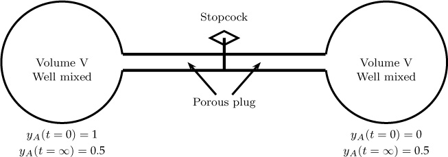
Diagrammatic illustration of the study of diffusion coefficient with two-bulb systems.

Figure 5.2 Two-bulb system for the study of diffusion coefficients. The entire system is at constant temperature and pressure.

Solution

To keep the total concentration in the bulk same, equal moles should counter-diffuse. Hence N_A = –N_B. N_t = 0, and υ* = 0.

The masses diffusing are not the same:

n_A = M_AN_A = 2N_A for hydrogen
n_B = M_BN_B = –28N_A for nitrogen

Hence

n_t = n_A + n_B = –26N_A

The net mass flow n_t is non-zero. The negative sign indicates that the flow is from the right side to the left side.

The corresponding velocity can be calculated as υ = n_t/ρ, with its value depending on the total density of the mixture. Note that υ is not zero.

The total density is different at the two ends. Hence the system velocity varies along the length and is directed toward the hydrogen side and increases as you approach the left bulb. Also note that the mass conservation concept requires ρv to be constant along the length.

Example 5.3 illustrates a case in which there is no mass averaged velocity but the molar average velocity is non-zero.

Example 5.3 Equimass Counter-Diffusion

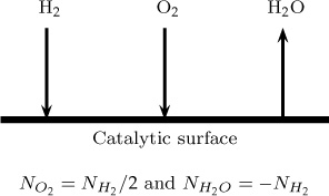
Consider hydrogen and oxygen diffusing to a catalytic surface. The product is water vapor, which diffuses back to the bulk gas (Figure 5.3). Assume 2 mmol/m² s hydrogen is diffusing to the catalyst at 1 atm total pressure and a temperature of 300 K. Show that υ is zero but not υ*.

Diagrammatic illustration of the problem related to Equimass Counter-Diffusion.

Figure 5.3 Diffusion followed by surface reaction to a catalytic surface.

Solution

By stoichiometry, we have the following relation between the fluxes since 2 moles of hydrogen reacts with 1 mole of oxygen to produce 2 moles of water:

Hydrogen: N_A = 2; oxygen: N_B = 1; water: N_C = –2. Units in mmol/m²s.

Total moles diffusing: N_t = 1

Total concentration: P/R_gT = 40 mol/m³

The velocity υ* can now be computed.

υ* = N_t/C = 1/40 = 2.5 × 10^–4 mm/s; a non-zero velocity.

Converting to mass units, we have n_A = 4; n_B = 32, n_c = –36 mg/m² s. Total n_t adds up to zero. Hence υ is zero.

To get the equation of mass transfer in the concentration C_A or partial density ρ_A form, we start with the flux form. Then n_A or N_A can be split into convection and diffusion terms and substituted into the flux form of the conservation model. This will provide us with the needed equations. Before we do this, it is useful to show some properties of the diffusive flux.

5.3 Properties of Diffusion Flux

Diffusion flux is defined in the moving frame, and this definition leads to some properties that are discussed next.

Property 1: The sum of the diffusive fluxes of all species is equal to zero.

This is proved as follows. Summing the definitions of diffusive flux of any species i given by Equation 5.12, we have

\begin{matrix} \sum J_{i} = \sum (C_{i} υ_{i}) - υ^{*} \sum C_{i} & (5.18) \end{matrix}

$\begin{matrix} \sum J_{i} = \sum (C_{i} υ_{i}) - υ^{*} \sum C_{i} & (5.18) \end{matrix}$

The summation of C_i is equal to the total concentration C and hence the previous equation can be written as

\begin{matrix} \sum J_{i} = \sum (C_{i} υ_{i}) - υ^{*} C & (5.19) \end{matrix}

$\begin{matrix} \sum J_{i} = \sum (C_{i} υ_{i}) - υ^{*} C & (5.19) \end{matrix}$

From the definition of mixture average velocity υ*, we note

\begin{matrix} υ^{*} C = (\sum_{i = 1}^{n s} y_{i} υ_{i}) C = \sum (C_{i} υ_{i}) & (5.20) \end{matrix}

$\begin{matrix} υ^{*} C = (\sum_{i = 1}^{n s} y_{i} υ_{i}) C = \sum (C_{i} υ_{i}) & (5.20) \end{matrix}$

The two terms on the right side of Equation 5.19 cancel out, proving that the sum of the diffusive flux taken over all the components is zero:

\begin{matrix} \begin{matrix} \sum_{i = 1}^{n s} J_{i} = 0 \end{matrix} & (5.21) \end{matrix}

$\begin{matrix} \begin{matrix} \sum_{i = 1}^{n s} J_{i} = 0 \end{matrix} & (5.21) \end{matrix}$

A similar equation also holds for j_A, the diffusion flux in mass units, and for Σ j_i = 0.

For example, in a binary system we have J_A = –J_B and there is only one independent diffusive flux. Likewise, for a multicomponent system there can be only (ns – 1) independent diffusive fluxes. Thus, in a ternary system containing species A, B, and C, the following equation holds:

J_C = –(J_A + J_B)

There can be only two independent diffusion fluxes.

Property 2: In a binary system, a single parameter D_AB is sufficient to model the diffusion flux.

The proof is as follows. Let there be two parameters, D_A and D_B. Then the flux for each species is proportional to its mole fraction gradient in the system:

\begin{matrix} J_{A} = - C D_{A} \frac{d y_{A}}{d z} & (5.22) \end{matrix}

$\begin{matrix} J_{A} = - C D_{A} \frac{d y_{A}}{d z} & (5.22) \end{matrix}$

and

\begin{matrix} J_{B} = - C D_{B} \frac{d y_{B}}{d z} & (5.23) \end{matrix}

$\begin{matrix} J_{B} = - C D_{B} \frac{d y_{B}}{d z} & (5.23) \end{matrix}$

For a binary system, the diffusive fluxes of A and B are related as follows:

J_A = –J_B

For a binary system:

y_A + y_B = 1

\frac{d y_{A}}{d z} + \frac{d y_{B}}{d z} = 0

$\frac{d y_{A}}{d z} + \frac{d y_{B}}{d z} = 0$

Hence it follows that

D_A = D_B = D_AB

Thus there is only one diffusion coefficient in a binary mixture, which is denoted as D_AB, the binary pair diffusion coefficient.

Property 3: In a multicomponent system, ns(ns – 1)/2) parameters are needed to model the diffusive fluxes.

This follows from Property 1. For example, in a three-component system there are only three independent diffusion fluxes. A model for flux can therefore be set up with the combination of three basic binary parameters: D_AB, D_BC, and D_AC. The Stefan-Maxwell equation, which we will study in Chapter 15, shows how the flux of each species can be related to these three basic binary parameters. A simpler model is to use the pseudo-binary diffusivity, which is discussed next.

5.4 Pseudo-Binary Diffusivity

Multicomponent diffusion does not follow Fick’s law; it is discussed in detail in Chapter 15. A simplified concept is that of pseudo-binary diffusivity, which is defined as follows:

J_A = –CD_A–mΔy_A

where D_A–m is the diffusivity of A in the mixture defined as though the system were a binary setup—the source of the name pseudo-binary diffusivity.

The multicomponent diffusion is treated as though the binary Fick’s law holds for each species taken individually. Note that this is only an approximation, but it turns out to be a good one if species A is present in dilute concentrations and diffusing in a mixture of B, C, . . ., and is mainly required to track the diffusion of species A only. In such cases, the Wilke (1950) equation is often used:

\begin{matrix} \frac{1 - y_{A}}{D_{A - m}} = \frac{y_{B}}{D_{A B}} + \frac{y c}{D_{A C}} + \dots & (5.24) \end{matrix}

$\begin{matrix} \frac{1 - y_{A}}{D_{A - m}} = \frac{y_{B}}{D_{A B}} + \frac{y c}{D_{A C}} + \dots & (5.24) \end{matrix}$

The calculation of the pseudo-binary diffusivity is shown in Example 5.4.

Example 5.4 Pseudo-Binary Diffusivity in a Ternary Mixture

Find the diffusivity of 10% CO₂ in an equimolar mixture of hydrogen and water. Use the Wilke equation.

Solution

The binary pair values are D₁₂ = 0.164 cm²/s and D₁₃ = 0.55 cm²/s. For an equimolar mixture, y₂ = y₃ = 0.45. Also y₁ = 0.1 as per the given data.

Hence from Equation 5.23, we obtain

\frac{1 - 0.1}{D_{A - m}} = \frac{0.45}{0.164} + \frac{0.45}{0.55}

$\frac{1 - 0.1}{D_{A - m}} = \frac{0.45}{0.164} + \frac{0.45}{0.55}$

Solving D_1–m = 0.2527 cm²/s. For this particular case, the diffusivity of species 1 in the mixture is the harmonic mean of that in species 2 and 3.

Note: The diffusivity calculated by the Wilke equation will be a function of the mixture composition; hence it is composition dependent. In practical applications, an average value based on an average mixture composition is used. The alternative is to use the more rigorous Stefan-Maxwell model discussed in Chapter 15. (This model was proposed independently by Stefan and Maxwell in 1871.)

5.5 Concentration Form

The basic differential equation for species mass transfer will now be derived. This section shows the derivations using the mass basis as well as the mole basis. The partial density ρ_A (same as mass concentration) is the field variable for the mass basis derivation, while the molar concentration C_A is the variable for the mole basis derivation.

5.5.1 Mass Basis

We repeat the mass conservation law derived earlier for convenience:

- ▽ \cdot n_{A} + r_{A} = \frac{\partial ρ_{A}}{\partial t}

$- ▽ \cdot n_{A} + r_{A} = \frac{\partial ρ_{A}}{\partial t}$

This is the basic differential species mass balance equation. Now since

n_A = υρ_A + j_A

as per Equation 5.7, the conservation equation can be written in terms of the diffusion flux (after moving some terms around):

\begin{matrix} \frac{\partial ρ_{A}}{\partial t} + \nabla \cdot (υ ρ_{A}) = - \nabla \cdot j_{A} + r A & (5.25) \end{matrix}

$\begin{matrix} \frac{\partial ρ_{A}}{\partial t} + \nabla \cdot (υ ρ_{A}) = - \nabla \cdot j_{A} + r A & (5.25) \end{matrix}$

The four terms represent the accumulation, convection, diffusion, and reaction.

If Fick’s law is used for j_A (which is strictly true for an ideal binary system), we obtain

\begin{matrix} \frac{\partial ρ_{A}}{\partial t} + \nabla \cdot (υ ρ_{A}) = \nabla \cdot (ρ D_{A} \nabla w A) + r A & (5.26) \end{matrix}

$\begin{matrix} \frac{\partial ρ_{A}}{\partial t} + \nabla \cdot (υ ρ_{A}) = \nabla \cdot (ρ D_{A} \nabla w A) + r A & (5.26) \end{matrix}$

5.5.2 Constant-Density Systems

For constant-density systems, we can move ρ inside the differentiation in Equation 5.25:

\begin{matrix} \frac{\partial ρ_{A}}{\partial t} + \nabla \cdot (υ ρ_{A}) = \nabla \cdot (D_{A} \nabla ρ_{A}) + r A & (5.27) \end{matrix}

$\begin{matrix} \frac{\partial ρ_{A}}{\partial t} + \nabla \cdot (υ ρ_{A}) = \nabla \cdot (D_{A} \nabla ρ_{A}) + r A & (5.27) \end{matrix}$

Liquid mixtures can often be approximated as constant-density systems. A gas mixture under isobaric and isothermal conditions with a small concentration of solute being transported can also be treated as constant-density system. Note that the density of a gas mixture is given as $\bar{M} P / R_{g} T$ $\bar{M} P / R_{g} T$ , where $\bar{M}$ $\bar{M}$ is the average molecular weight. For mixtures with a small concentration of diffusing solute, the contribution to $\bar{M}$ $\bar{M}$ from the changes in solute concentration is small; thus such mixtures can be treated as constant-density case.

If the diffusion coefficient is constant, the first term on the right side of Equation 5.27 can be expressed in Laplacian terms:

\begin{matrix} \frac{\partial ρ_{A}}{\partial t} + \nabla \cdot (υ ρ_{A}) = D_{A} \nabla^{2} ρ_{A} + r A & (5.28) \end{matrix}

$\begin{matrix} \frac{\partial ρ_{A}}{\partial t} + \nabla \cdot (υ ρ_{A}) = D_{A} \nabla^{2} ρ_{A} + r A & (5.28) \end{matrix}$

This is the equation on a mass basis. Note that the reference velocity is υ here.

Dividing by M_A we get the molar form:

\begin{matrix} \frac{\partial C_{A}}{\partial t} + \nabla \cdot (υ C_{A}) = D_{A} \nabla^{2} C_{A} + R_{A} & (5.29) \end{matrix}

$\begin{matrix} \frac{\partial C_{A}}{\partial t} + \nabla \cdot (υ C_{A}) = D_{A} \nabla^{2} C_{A} + R_{A} & (5.29) \end{matrix}$

Note that r_A/M_A is replaced by R_A in arriving at this equation.

Equation 5.29 is commonly used to obtain species concentration for mass transfer analysis. Indeed, many applications studied in later chapters use this equation as a starting point. Note that the assumption of constant mixture density is implied in its derivation.

5.5.3 Overall Continuity: Mass Basis

If Equation 5.25 is summed over all the species, we obtain the overall mass balance, also known as the continuity equation. We note the following properties and use it in summation:

Σρ_A = ρ, the mixture density
Σj_A = 0; the property of diffusion flux
Σr_A = 0; no total mass is formed by reaction

The overall continuity is then

\begin{matrix} \frac{\partial ρ}{\partial t} + \nabla \cdot (υ ρ) = 0 & (5.30) \end{matrix}

$\begin{matrix} \frac{\partial ρ}{\partial t} + \nabla \cdot (υ ρ) = 0 & (5.30) \end{matrix}$

This is same as the continuity equation derived in fluid mechanics.

For constant-density systems, Equation 5.30 reduces to

∇ · υ = 0

This is known as the incompressibility condition in fluid mechanics. Using this definition in Equation 5.26, we have

\begin{matrix} \frac{\partial ρ_{A}}{\partial t} + υ \cdot \nabla ρ_{A} = \nabla \cdot (D_{A} \nabla ρ_{A}) + r A & (5.31) \end{matrix}

$\begin{matrix} \frac{\partial ρ_{A}}{\partial t} + υ \cdot \nabla ρ_{A} = \nabla \cdot (D_{A} \nabla ρ_{A}) + r A & (5.31) \end{matrix}$

5.5.4 Mole Basis

Now we will repeat the same model derivations but on a mole basis. We will also use the molar average velocity υ* as the reference velocity.

We repeat the mass conservation law derived earlier for convenience:

- \nabla \cdot N_{A} + R_{A} = \frac{\partial C_{A}}{\partial t}

$- \nabla \cdot N_{A} + R_{A} = \frac{\partial C_{A}}{\partial t}$

This is the basic differential species mass balance equation. Now since

N_A = υ*C_A + J_A

as per Equation 5.14, the equation can be written in terms of the diffusion flux as

\begin{matrix} \frac{\partial C_{A}}{\partial t} + \nabla \cdot (υ^{*} C_{A}) = - \nabla \cdot J_{A} + R_{A} & (5.32) \end{matrix}

$\begin{matrix} \frac{\partial C_{A}}{\partial t} + \nabla \cdot (υ^{*} C_{A}) = - \nabla \cdot J_{A} + R_{A} & (5.32) \end{matrix}$

If Fick’s law is used for J_A (which is strictly true for an ideal binary system), we obtain

\begin{matrix} \frac{\partial C_{A}}{\partial t} + \nabla \cdot (υ^{*} C_{A}) = \nabla \cdot (C D_{A} \nabla y_{A}) + R_{A} & (5.33) \end{matrix}

$\begin{matrix} \frac{\partial C_{A}}{\partial t} + \nabla \cdot (υ^{*} C_{A}) = \nabla \cdot (C D_{A} \nabla y_{A}) + R_{A} & (5.33) \end{matrix}$

For constant concentration conditions and the constant diffusivity case, we obtain

\begin{matrix} \frac{\partial C_{A}}{\partial t} + \nabla \cdot (υ^{*} C_{A}) = D_{A} \nabla^{2} C_{A} + R_{A} & (5.34) \end{matrix}

$\begin{matrix} \frac{\partial C_{A}}{\partial t} + \nabla \cdot (υ^{*} C_{A}) = D_{A} \nabla^{2} C_{A} + R_{A} & (5.34) \end{matrix}$

5.5.5 Overall Continuity: Mole Basis

We now derive an overall continuity equation based on the mole basis and point out the difference between this equation and that obtained on a mass basis. The starting point is to sum Equation 5.32 over all the species. The sum of the diffusion fluxes remains zero. Although Σ_i J_i = 0, Σ_i R_i may not be equal to zero.

Summing Equation 5.32 over all the species, we get the mole continuity equation:

\frac{\partial C}{\partial t} + \nabla \cdot (υ^{*} C) = \sum_{i} R_{i}

$\frac{\partial C}{\partial t} + \nabla \cdot (υ^{*} C) = \sum_{i} R_{i}$

If there is no net change in the number of moles in the balanced chemical reaction, then Σ_i R_i = 0—for example, if A + B gives C + D. More generally, we note that the following equation holds if a single reaction is taking place:

\sum R_{i} = (\sum ν_{i}) R

$\sum R_{i} = (\sum ν_{i}) R$

Here ν_i is the stoichiometric coefficient for the ith species. $R$ $R$ is a rate function that measures the rate of production (defined as the rate of a product species with unit stoichiometry—that is, as R_A/ν_A). If Σν_i is equal to zero (there is no net change in the total moles), the ΣR_i term will be equal to zero. Otherwise, this term should be retained in the overall mole continuity equation.

5.5.6 Common Simplifications

The commonly used governing equation for mass transfer is restated here for ease of reference:

\begin{matrix} \begin{matrix} \frac{\partial C_{A}}{\partial t} + υ \cdot ▽ C_{A} = D_{A} ▽^{2} C_{A} + R_{A} \end{matrix} & (5.35) \end{matrix}

$\begin{matrix} \begin{matrix} \frac{\partial C_{A}}{\partial t} + υ \cdot ▽ C_{A} = D_{A} ▽^{2} C_{A} + R_{A} \end{matrix} & (5.35) \end{matrix}$

This equation applies to a constant-density system and is used as a starting point to solve many mass transfer problems. The four terms in this equation represent accumulation, convection, diffusion, and reaction. Depending on which of these terms balance, the equation can be simplified. The solutions of some prototypical problems with these simplifications are studied in later chapters.

For pure diffusion problems, Equation 5.35 reduces to

Δ²C_A = 0

This model applies when there is no superimposed flow and when the diffusion-induced velocity is zero or can be neglected.

Diffusion-induced convection problems may be approached with the following form of Equation 5.35:

∇ · N_A = 0 for A, B, C, . . .

where N_A is given by Equation 5.14. Some additional problem-specific conditions needs to be superimposed to obtain the total flux N_t = N_A + N_B + ... on the system.

Both pure diffusion and diffusion-induced convection problems are examined in Chapter 6.

For transient diffusion with no reaction, the differential equation reduces to Fick’s second law:

\begin{matrix} \frac{\partial C_{A}}{\partial t} = D_{A} \nabla^{2} C_{A} & (5.36) \end{matrix}

$\begin{matrix} \frac{\partial C_{A}}{\partial t} = D_{A} \nabla^{2} C_{A} & (5.36) \end{matrix}$

which states that the accumulation balances the net diffusion from the control surfaces. The solutions to illustrative problems are presented in Chapter 8.

In convection–diffusion problems, the diffusion term is balanced by the convection term, leading to the following simplified version of the general differential equation:

\begin{matrix} υ \cdot \nabla C_{A} = D_{A} \nabla^{2} C_{A} & (5.37) \end{matrix}

$\begin{matrix} υ \cdot \nabla C_{A} = D_{A} \nabla^{2} C_{A} & (5.37) \end{matrix}$

which states that convection balances diffusion. A velocity profile has to be prescribed to proceed further. These types of problems are addressed in Chapters 10 and 11.

In diffusion–reaction problems, the diffusion term is balanced by the rate of production. This leads to the following governing equation:

\begin{matrix} D_{A} \nabla^{2} C_{A} + R_{A} = 0 & (5.38) \end{matrix}

$\begin{matrix} D_{A} \nabla^{2} C_{A} + R_{A} = 0 & (5.38) \end{matrix}$

which states that the net diffusion balances the rate of production. Diffusion with reaction is studied in more detail in Chapters 18 and 20.

5.6 Common Boundary Conditions

Boundary conditions for mass transfer are generally classified into three types:

Dirichlet: This applies if the concentration is specified at a point in the boundary. It is also known as the boundary condition of the first kind.
Neumann: This applies if the slope of concentration is specified at a point in the boundary. It is also known as the boundary condition of the second kind.
Robin: In this type, neither the concentration nor its slope is specified, but rather some relation connecting the two is specified. It is also known as the boundary condition of the third kind.

We now illustrate the various common cases and indicate what the appropriate boundary conditions are for these cases.

At the interface (such as a dissolving solid surface), the concentration can be prescribed. Concentration in the liquid will be the saturation solubility of the solid. This leads to a Dirichlet type of condition.
At a plane of symmetry or an impermeable wall, the flux is equal to zero, leading to a Neumann condition. Here, dC_A/dn is specified as zero.
At a heterogeneous surface where a surface reaction occurs, a Robin condition results. The rate of diffusion N_A is equated to the rate of surface reaction –R_A,s here:

N_A = –R_A,s

If Fick’s law is used for N_A and a first-order reaction takes place at the surface, so that

R_A,s = –k_sC_A

then the boundary condition to be used is

$\begin{matrix} - D_{A} \frac{d C_{A}}{d n} = k_{s} C_{A} at the surface & (5.39) \end{matrix}$ $\begin{matrix} - D_{A} \frac{d C_{A}}{d n} = k_{s} C_{A} at the surface & (5.39) \end{matrix}$

This can be seen as a boundary condition of the third kind (Robin condition). Here n is the direction toward the surface. Neither the concentration value nor the flux value is specified, but the relation in Equation 5.39 ties the two together. Hence the third kind of boundary condition is a mixed boundary condition.
A limiting case for the heterogeneous reaction is a fast reaction at the surface. The concentration of the limiting reactant is set as zero for this case and the Dirichlet condition is used. Note that the concentration cannot be actually equal to zero, since then there would be no reaction. The zero value should be conceived as a limit when the rate constant k_s tends to infinity in Equation 5.39.
At a gas–liquid interface, the concentration jump condition is used, but the fluxes are continuous at this surface. Thus N_Ai from the gas side is equal to N_Ai into the liquid (i means the interface here), while the concentration C_Ai at the interface on the gas side is related to C_Ai on the liquid side by an equilibrium constant or Henry’s law constant.
If the solid is in contact with a fluid, the flux by diffusion from the solid is equal to the convective transport from the solid surface to the bulk of the fluid. A Robin boundary condition is therefore used at the solid–fluid interface where a convective transport is taking place:

$- D_{A} \frac{d C_{A}}{d x} = k_{m} (H_{A} C_{A} - C_{A b})$ $- D_{A} \frac{d C_{A}}{d x} = k_{m} (H_{A} C_{A} - C_{A b})$

with H_A being the Henry’s law constant that relates the concentration in the solid phase to that in the fluid, k_m is the mass transfer coefficient, and C_Ab is the concentration in the fluid away from the solid (i.e., the bulk concentration).

These scenarios cover most of the commonly encountered boundary conditions in mass transfer problems.

5.7 Macroscopic Models: Single-Phase Systems

This section may be omitted with no loss of continuity.

This section provides the derivation of the macroscopic model used in mass transfer analysis by volume averaging of the differential equations of mass transport. Working models for design of mass transfer equipment are often based on such macroscopic models. Single-phase systems are shown here. Extension to multiphase systems requires some additional concepts of local volume averaging and is briefly discussed in the next section.

The starting point is integration of the differential equation given by Equation 5.2, which is reproduced here for ease of reference:

\begin{matrix} - \nabla \cdot N_{A} + R_{A} = \frac{\partial C_{A}}{\partial t} & (5.40) \end{matrix}

$\begin{matrix} - \nabla \cdot N_{A} + R_{A} = \frac{\partial C_{A}}{\partial t} & (5.40) \end{matrix}$

This equation is integrated over a macroscopic control volume, which leads to the macroscopic species balance:

\begin{matrix} - \int_{V} (\nabla \cdot N_{A}) d V + \int_{V} R_{A} d V = \int_{V} (\frac{\partial C_{A}}{\partial t}) d V & (5.41) \end{matrix}

$\begin{matrix} - \int_{V} (\nabla \cdot N_{A}) d V + \int_{V} R_{A} d V = \int_{V} (\frac{\partial C_{A}}{\partial t}) d V & (5.41) \end{matrix}$

We show the representation of each of these terms in the following paragraphs. The first term in Equation 5.41 is the combined flux term. To integrate this, we need the divergence theorem, also known as the Green-Gauss theorem in vector calculus. This theorem says that a surface integral can be converted to a volume integral. We use this idea in reverse to convert the volume integral to a surface integral:

\begin{matrix} - \int_{V} (\nabla \cdot N_{A}) d V = - \int_{S} (n \cdot N_{A}) d S & (5.42) \end{matrix}

$\begin{matrix} - \int_{V} (\nabla \cdot N_{A}) d V = - \int_{S} (n \cdot N_{A}) d S & (5.42) \end{matrix}$

The second term in Equation 5.41 is the reaction rate term ∫V R_AdV . It can also be written as V 〈R_A〉, where 〈R_A〉 is the average rate of reaction defined as

〈 R_{A} 〉 = \frac{1}{V} \int_{V} R_{A} d V

$〈 R_{A} 〉 = \frac{1}{V} \int_{V} R_{A} d V$

Finally, the accumulation term on the right side of Equation 5.41 can be written as

accumulation = \int_{υ} \frac{\partial C_{A}}{\partial t} d V

$accumulation = \int_{υ} \frac{\partial C_{A}}{\partial t} d V$

This expression can be rewritten as follows, assuming that the control volume is not changing in time:

accumulation = \frac{d}{d t} (\int_{υ} C_{A} d V)

$accumulation = \frac{d}{d t} (\int_{υ} C_{A} d V)$

In turn, this expression can be written in terms of an average concentration:

accumulation = \frac{d}{d t} (V 〈 C_{A}))

$accumulation = \frac{d}{d t} (V 〈 C_{A}))$

where we use the following definition:

〈 C_{A} 〉 = \frac{1}{V} \int_{V} C_{A} d V

$〈 C_{A} 〉 = \frac{1}{V} \int_{V} C_{A} d V$

Combining all the terms, we obtain the macroscopic species balance equation:

\begin{matrix} \begin{matrix} - \int_{S} (n \cdot N_{A}) d S + V 〈 R_{A} 〉 = \frac{d}{d t} (V 〈 C_{A} 〉) \end{matrix} & (5.43) \end{matrix}

$\begin{matrix} \begin{matrix} - \int_{S} (n \cdot N_{A}) d S + V 〈 R_{A} 〉 = \frac{d}{d t} (V 〈 C_{A} 〉) \end{matrix} & (5.43) \end{matrix}$

We can compare Equation 5.43 with the macroscopic balance shown earlier in Chapter 2, which is repeated here for ease of reference:

\begin{matrix} {\dot{M}}_{A, i} - {\dot{M}}_{A, e} - {\dot{M}}_{A, W} + V 〈 R_{A} 〉 = \frac{d}{d t} (M_{A}) & (5.44) \end{matrix}

$\begin{matrix} {\dot{M}}_{A, i} - {\dot{M}}_{A, e} - {\dot{M}}_{A, W} + V 〈 R_{A} 〉 = \frac{d}{d t} (M_{A}) & (5.44) \end{matrix}$

The reaction terms and the accumulation terms are the same as in Equation 5.43 since V 〈C_A〉 = $M$ $M$ _A.

The first three terms in Equation 5.44 can be formally established if the control surface is split into an inlet region S_i, an outlet region S_e, the permeable wall or interface S_w, and the impermeable walls S_im:

S = S_i + S_e + S_W + S_im

The surface integral term in Equation 5.43 is evaluated for each of these regions. The corresponding contributions of these integrals lead to the moles crossing the inlet region of the overall control surface, leaving the outlet part and the amount transferred to walls or to an interface or membrane.

For illustration, at the inlet the flux vector is mainly convective and can be approximated as υC_A. The inlet contribution of the integral in Equation 5.43 is

–∫S_i (n · N_A) dS = ∫S_i (n · υC_A) dS = S_i 〈vC_A〉

Here υ (with no boldface) represents the velocity component in the direction of the inlet flow. (This is equal to –n · υ since the normal direction n is usually chosen outward from the control volume.) Hence the inlet contribution can be represented as S_i 〈vC_A〉, and is seen to be the moles of A entering the inlet region, ${\dot{M}}_{A, i}$ ${\dot{M}}_{A, i}$ (the first term in Equation 5.44). The cup mixed average appears naturally as the representative concentration for the inlet (and outlet) streams.

Similar considerations apply for the integral over the exit region S_e and lead to the $- {\dot{M}}_{A, e}$ $- {\dot{M}}_{A, e}$ term.

The permeable walls flux term likewise leads to the $- {\dot{M}}_{A, w}$ $- {\dot{M}}_{A, w}$ term if one identifies this term as the surface integral of the local flux vector:

{\dot{M}}_{A, w} = \int_{S_{w}} (n \cdot N_{A}) d S

${\dot{M}}_{A, w} = \int_{S_{w}} (n \cdot N_{A}) d S$

Finally, the integral over the impermeable wall region is zero. Thus the first three terms in Equation 5.44 are the integrals of the corresponding flux components, and the macroscopic balance is derived by a formal integration of the differential balance.

5.8 Multiphase Systems: Local Volume Averaging

This section may be omitted with no loss of continuity.

The basis for the differential model for two-phase systems remains to be clarified. This section shows the basis for this model using the concept of local volume averaging.

The analysis presented here is somewhat advanced and not often covered in the undergraduate curriculum. The material will be useful to follow some current literature on this topic, and for understanding the basic ideas used in the CFD (computational fluid dynamics) model of mass transfer in multiphase systems. Hence the goal of this section is to provide an introductory background that supports further study in this field.

In a multiphase system, two phases flow past each other. One phase is usually dispersed in the other phase, and any selected control volume will contain both phases (Figure 5.4). We denote the phases as c and d. The species conservation law applies locally within each phase. Thus, for the dispersed phase:

\begin{matrix} \frac{\partial C_{A d}}{\partial t} + \nabla \cdot N_{A d} = R_{A d} & (5.45) \end{matrix}

$\begin{matrix} \frac{\partial C_{A d}}{\partial t} + \nabla \cdot N_{A d} = R_{A d} & (5.45) \end{matrix}$

Diagrammatic representation of a multiphase system, containing two phases.

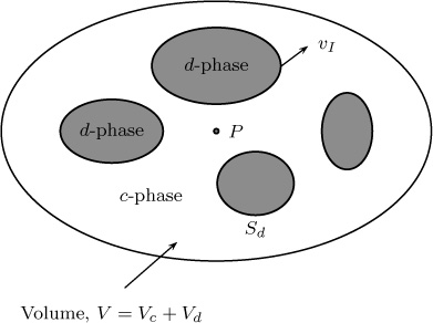
Figure 5.4 Local control volume showing two interacting phases and an averaging surface associated with any point P · S_d is the total surface area between the c-phase and d-phase within the volume. v_I is the relative velocity with which the surface of the dispersed phase may be moving.

where the subscript d indicates that all quantities are applicable within the dispersed phase. A similar equation holds for the continuous phase (not shown for brevity).

If the precise locations of the phases are known, these equations can be solved with the boundary conditions applied at the interface between the two phases. The boundary conditions are the flux continuity and the concentration jump at the interface. Examples of such cases include annular flow in a pipe, slug flow in a microchannel, and a falling film reactor. The two phases are segregated in these cases, and the species continuity equation can be solved for each phase, although this may be computationally intensive and challenging in some situations.

If the phases are dispersed as shown in Figure 5.4, the approach of solving each phase separately is not useful because this is now a dynamic system: The precise location of the interface is not known and may be changing with time. Solution of such a deterministic multiboundary problem is difficult. Some simplification is needed, which is provided by local volume averaging.

Averaging volume V is composed of V_c and V_d—that is, the volumes occupied by phases 1 and 2. Likewise, the averaging surface S consists of S_c and S_d.

The local volume average for the dispersed phase is defined as

\begin{matrix} \bar{C_{A d}} = \frac{1}{V} \int_{V_{d}} C_{A d} d V & (5.46) \end{matrix}

$\begin{matrix} \bar{C_{A d}} = \frac{1}{V} \int_{V_{d}} C_{A d} d V & (5.46) \end{matrix}$

A similar definition applies for the continuous phase as well. Here V_d is the volume occupied by the dispersed phase and V is a local total volume over which averaging is done.

We can also define an intrinsic volume average:

\begin{matrix} {\tilde{C}}_{A d} = \frac{1}{V_{d}} \int_{V_{d}} C_{A d} d V & (5.47) \end{matrix}

$\begin{matrix} {\tilde{C}}_{A d} = \frac{1}{V_{d}} \int_{V_{d}} C_{A d} d V & (5.47) \end{matrix}$

The two local averages and the intrinsic average are related as follows:

\begin{matrix} \bar{C_{A d}} = ɛ_{d} {\tilde{C}}_{A d} & (5.48) \end{matrix}

$\begin{matrix} \bar{C_{A d}} = ɛ_{d} {\tilde{C}}_{A d} & (5.48) \end{matrix}$

where ∊_d is the volume fraction of the dispersed phase.

ɛ_{d} = \frac{V_{d}}{V}

$ɛ_{d} = \frac{V_{d}}{V}$

Hence the volume averaged continuity is

\begin{matrix} \bar{\frac{\partial C_{A d}}{\partial t}} + \bar{\nabla \cdot N_{A d}} = \bar{R_{A d}} & (5.49) \end{matrix}

$\begin{matrix} \bar{\frac{\partial C_{A d}}{\partial t}} + \bar{\nabla \cdot N_{A d}} = \bar{R_{A d}} & (5.49) \end{matrix}$

To perform further manipulations, we need two theorems for volume average of the time derivative and divergence. These concepts are often referred to as Gray’s (1975, 1983) theorem for volume averaging. (The theorem is on off-shoot of earlier papers by Slattery (1969) and Whitaker, 1969.)

Theorem for volume average of vector operations

Volume average of the time derivative of a scalar:

$\begin{matrix} \bar{\frac{\partial C_{A}}{\partial t}} = \frac{\partial \bar{C_{A}}}{\partial t} - \frac{1}{V} \int_{S_{d}} C_{A} (υ_{I} \cdot n) d S & (5.50) \end{matrix}$ $\begin{matrix} \bar{\frac{\partial C_{A}}{\partial t}} = \frac{\partial \bar{C_{A}}}{\partial t} - \frac{1}{V} \int_{S_{d}} C_{A} (υ_{I} \cdot n) d S & (5.50) \end{matrix}$

where v_I is the relative velocity with which the interface between c and d is moving.
Divergence of a vector:

$\begin{matrix} \bar{\nabla \cdot N_{A}} = \nabla \cdot \bar{N_{A}} + \frac{1}{V} \int_{S_{d}} N_{A} \cdot n d S & (5.51) \end{matrix}$ $\begin{matrix} \bar{\nabla \cdot N_{A}} = \nabla \cdot \bar{N_{A}} + \frac{1}{V} \int_{S_{d}} N_{A} \cdot n d S & (5.51) \end{matrix}$

The first term in Equation 5.49 is the average of the time derivative of the average concentration. It is equal to the time derivative of the average concentration if the control surface of the dispersed phase is not changing with time. This will apply, for example, to dilute systems where the drop or the bubble size is not changing much during mass transfer. Otherwise, an extra term that includes the relative velocity of the interface (shown in Equation 5.50) must be taken into account.

The second term in Equation 5.49 is the volume average of the divergence. This is not equal to the divergence of the volume average, so the extra surface integral shown in Equation 5.51 must be added according to Gray’s theorem.

The use of these theorems in Equation 5.49 then leads to the following expression:

\begin{matrix} \begin{matrix} \frac{\partial \bar{C_{A d}}}{\partial t} + \nabla \cdot \bar{N_{A d}} = \bar{R_{A d}} - \frac{1}{V} \int_{S_{d}} (N_{A} \cdot n) d S \\ + \frac{1}{V} \int_{S_{d}} C_{A} (υ_{I} \cdot n) d S = 0 \end{matrix} & (5.52) \end{matrix}

$\begin{matrix} \begin{matrix} \frac{\partial \bar{C_{A d}}}{\partial t} + \nabla \cdot \bar{N_{A d}} = \bar{R_{A d}} - \frac{1}{V} \int_{S_{d}} (N_{A} \cdot n) d S \\ + \frac{1}{V} \int_{S_{d}} C_{A} (υ_{I} \cdot n) d S = 0 \end{matrix} & (5.52) \end{matrix}$

The last two terms are interpreted as the interfacial transfer term and the contribution due to change in volume of the dispersed phase due to shrinkage or growth. Note that the interface mass transfer term arises automatically as a consequence of local volume averaging combined with the use of Gray’s theorem. The interfacial term is represented as the transfer rate ${\dot{M}}_{d c}$ ${\dot{M}}_{d c}$ from the dispersed phase to the continuous phase per unit volume:

{\dot{M}}_{d c} = \int_{S_{d}} N_{A} \cdot n d S

${\dot{M}}_{d c} = \int_{S_{d}} N_{A} \cdot n d S$

The use of these theorems in Equation 5.49 leads to the local volume averaged model for the dispersed phase:

\begin{matrix} \frac{\partial \bar{C_{A d}}}{\partial t} + \nabla \cdot \bar{N_{A d}} = \bar{R_{A d}} - \frac{{\dot{M}}_{d c}}{V} & (5.53) \end{matrix}

$\begin{matrix} \frac{\partial \bar{C_{A d}}}{\partial t} + \nabla \cdot \bar{N_{A d}} = \bar{R_{A d}} - \frac{{\dot{M}}_{d c}}{V} & (5.53) \end{matrix}$

where we have omitted the shrinkage/expansion term. This model assumes constant drop diameter, for instance.

The corresponding equation for the continuous phase completes the model:

\begin{matrix} \frac{\partial \bar{C_{A c}}}{\partial t} + \nabla \cdot \bar{N_{A c}} = \bar{R_{A c}} + \frac{{\dot{M}}_{d c}}{V} & (5.54) \end{matrix}

$\begin{matrix} \frac{\partial \bar{C_{A c}}}{\partial t} + \nabla \cdot \bar{N_{A c}} = \bar{R_{A c}} + \frac{{\dot{M}}_{d c}}{V} & (5.54) \end{matrix}$

Note that the mass transfer term now appears with a plus sign the direction of the unit normal is toward the dispersed phase.

It may be useful to summarize the various length scales involved and evaluate the local volume average on this basis. The following length scales are readily identified:

Dispersed phase scale, d (e.g., bubble or drop diameter or particle diameter)
Scale of averaging volume, r
Total length scale (e.g., reactor or vessel diameter), L

The local volume averaging assumption assumes d < r < L. In other words, the averaging volume should include several particles of the dispersed phase but should be much smaller than the overall reactor length scale. Therefore, unless we are dealing with a highly dispersed system, the control volume cannot be reduced to an infinitesimal volume. This constraint is one difficulty in using this approach. Similarly, the rate of mass transfer depends on the the local velocity and local diffusion flux at the interface, which is not available from a volume averaged model. The volume averaging blurs the lines between the two phases and treats them as an interpenetrating continuum. Hence the equations must be supplemented with some transport model; commonly one defines and uses the local mass transfer coefficient for this purpose.

If each phase equation is now further averaged over a larger control volume, the two-phase macroscopic or mesoscopic models are obtained. This provides a formal way of developing the equation, identifies the information loss due to averaging, and suggests the required closures.

Summary

The application of the mass conservation law to a species leads to the differential equation for mass transfer. Such equations can be written in either mass units or mole units. Mole units are more convenient for reactive systems.
The differential equations based on the conservation law must be supplemented with a model for diffusion flux to obtain the corresponding equations in the concentration form. A definition of the mixture velocity is needed to model the diffusion flux.
In a multicomponent mixture, a velocity can be associated with each species. The velocity is related to the fluxes in a stationary frame of reference. One can use mole or mass units freely here and convert from one set to the other.
Averaging the species velocities gives us a value for the velocity of the mixture as a whole. However, there is no unique way of averaging, which leads to many definitions for this average velocity and the corresponding definitions for the diffusion flux.
Two common ways of averaging are based on use of either the mass fraction or the mole fraction as the weighting factor. The results are the mass averaged and mole averaged velocities for the system. The notations υ and υ*, respectively, are commonly used for these quantities.
A flux—the diffusion flux—can be defined based on a coordinate system moving with either of these average velocities. Thus we can have a diffusion flux based on mass averaged velocity as a reference frame (j_A) or a diffusion flux based on mole averaged frame (J_A).
In a binary mixture, there is only one independent diffusion flux although there are two components: j_B = –j_A in mass units or J_B = –J_A in mole units. In a multicomponent system, the sum of the diffusion fluxes taken for all the species is zero. Thus, in a ternary system, there are only two independent diffusion fluxes.
Constitutive equations relate diffusion fluxes to the concentration gradient or, more generally, to the mole (or mass) fraction gradient. Fick’s law is often suitable for binary systems or used as an approximation even for multicomponent systems. Depending on the frame of reference used to define diffusion flux, Fick’s law can take different forms. The most common form relates J_Ax to dC_A/dx; this variant is used for isothermal and isobaric systems.
The use of the diffusion flux permits us to develop differential equations of mass transfer in concentration form.
The boundary conditions to be used in the differential equation can be classified as being of the Dirichlet, Neumann, or Robin type.
At the phase interface, fluxes are matched on either side, while a concentration jump condition consistent with thermodynamic equilibrium is imposed for the concentrations.
The integration of the differential models over an arbitrary control volume leads to the macroscopic mass balance models discussed in Chapter 3. Although the macroscopic models can be written starting from the basic conservation law, this averaging approach is more elegant and provides the link between differential and macroscopic models. It also provides a precise definition of all the terms appearing in the macroscopic model.
Differential models for two-phase systems can be obtained by a procedure called local volume averaging. The mass exchange term between the two phases arises automatically by this procedure (which has to be closed by a transport law). The derived equations are applied locally for each phase at any given point; that is, the phases are assumed to be an interpenetrating continuum. If these “pointwise” models are averaged over a larger volume, then the macroscopic or mesoscopic two-phase models can be derived from first principles.

Review Questions

5.1 Is n_A equal to M_AN A? Why?

5.2 Is $j_{A}^{(m)}$ $j_{A}^{(m)}$ equal to $M_{A} j_{A}^{*}$ $M_{A} j_{A}^{*}$ Why?

5.3 State a (diffusion) problem where both υ and υ* are non-zero.

5.4 State a (diffusion) problem where υ is non-zero but υ* is zero.

5.5 State a (diffusion) problem where υ is zero but υ* is non-zero.

5.6 State a (diffusion) problem where both υ and υ* are zero.

5.7 In Example 5.1, does υ* change with distance along the vapor space? Does υ change?

5.8 When is ΣR_j equal to zero?

5.9 State equations for divergence of υ and divergence of υ*.

5.10 How does the overall mole continuity equation simplify for the steady state and no change in moles in the reaction?

5.11 Are the fluxes the same on both sides of a gas–liquid interface? What about the concentrations?

5.12 How can mesocopic models be derived when starting from differential models?

5.13 What is meant by local volume averaging?

5.14 What is Gray’s theorem, and when is it useful?

Problems

5.1 Divergence of the flux vector interpretation. If N_A is a flux vector at any point on the control surface and n is the unit normal outward from the surface, interpret the term NA · n. If dA is a differential area of surface at this point, write an expression for the mole efflux from this differential area. Then show that

Net moles efflux from the control surface = \int_{A} (N_{A} \cdot n) d A

$Net moles efflux from the control surface = \int_{A} (N_{A} \cdot n) d A$

Convert the area integration to a volume integral by using the Gauss divergence theorem. If the control volume now tends to zero, show that mole efflux per unit volume is equal to the divergence of the flux vector.

5.2 Combined flux: r-diffusion only in cylinder and sphere. How does the equation shown for the divergence operator in the text simplify to a case with cylindrical coordinates and diffusion only when there is only variation in the r-direction? Compare your answer with the result in Chapter 2.

How does the equation for the divergence simplify to a case with spherical coordinates and diffusion when there is only variation in the r-direction? Compare your answer with the result in Chapter 2.

5.3 Comparison of υ and υ*: A gas mixure consists of hydrogen and nitrogen. The combined flux vector of hydrogen at a point is 10 mmol/m² s, where the gas composition is 20% by moles of hydrogen. The flux of nitrogen is zero. Calculate υ and υ* at this point. Total pressure is 1 atm and temperature is 300 K.

5.4 Relation between species velocities. Show the following relations between the species velocities v_A and v_B referred to a stationary frame of reference:

υ_{A} - υ_{B} = j_{A} (\frac{1}{ρ_{A}} + \frac{1}{ρ_{B}})

$υ_{A} - υ_{B} = j_{A} (\frac{1}{ρ_{A}} + \frac{1}{ρ_{B}})$

υ_{A} - υ_{B} = j_{B} (\frac{1}{C_{A}} + \frac{1}{C_{B}})

$υ_{A} - υ_{B} = j_{B} (\frac{1}{C_{A}} + \frac{1}{C_{B}})$

5.5 Velocity variation with position in the two-bulb apparatus. In the two-bulb experiment shown in Figure 5.2, the porous plug is 1 m long and the diffusion coefficient is 7.0 × 10^–5 m²/s. The left bulb contains hydrogen and the right bulb contains nitrogen. Calculate and plot υ as a function of length along the porous plug.

5.6 Relation between j_A and J_A for a binary system. Show that the following relationship holds for a binary mixture:

j_{A} = \frac{M_{A} M_{B}}{\bar{M}} J_{A}

$j_{A} = \frac{M_{A} M_{B}}{\bar{M}} J_{A}$

5.7 Alternative forms of Fick’s law. Derive the following form of Fick’s law:

j_{A} = - \frac{C^{2}}{ρ} M_{A} M_{B} D_{A B} \nabla y_{A}

$j_{A} = - \frac{C^{2}}{ρ} M_{A} M_{B} D_{A B} \nabla y_{A}$

where y_A is the mole fraction. Show that this can also be expressed as

j_{A} = - C \frac{M_{A} M_{B}}{\bar{M}} D_{A B} \nabla y_{A}

$j_{A} = - C \frac{M_{A} M_{B}}{\bar{M}} D_{A B} \nabla y_{A}$

5.8 Inverted form of Fick’s law. For a binary mixture, derive the following equation based on Fick’s law:

\begin{matrix} \nabla x_{A} = \frac{x_{A} N_{B} - x_{B} N_{A}}{C D_{A B}} & (5.55) \end{matrix}

$\begin{matrix} \nabla x_{A} = \frac{x_{A} N_{B} - x_{B} N_{A}}{C D_{A B}} & (5.55) \end{matrix}$

Show that the following equation holds as well:

\begin{matrix} \nabla x_{A} = \frac{x_{A} J_{B} - x_{B} J_{A}}{C D_{A B}} & (5.56) \end{matrix}

$\begin{matrix} \nabla x_{A} = \frac{x_{A} J_{B} - x_{B} J_{A}}{C D_{A B}} & (5.56) \end{matrix}$

These are inverted forms; that is, they make flux implicit. Extension of these equations to multicomponent systems leads directly to the Stefan-Maxwell equation.

5.9 Volume fraction weighting. Mole fraction and mass fraction are commonly used weighting factors to find the mixture velocity. Volume fraction φ_υ can also be used as the weighting factor and one can define the average velocity v^V as follows:

υ^{y} = \sum φ_{υ} υ_{i}

$υ^{y} = \sum φ_{υ} υ_{i}$

Verify that the volume fraction averaged velocity is the same as the mole fraction averaged velocity when the total molar concentration (molar density) is constant (e.g., in a gas mixture).

Verify that volume fraction averaged velocity is the same as the mass fraction averaged velocity when the total mass density is constant (e.g., in a liquid mixture).

Derive a form of Fick’s law based on this definition of average velocity for a binary mixture.

Also show that the sum of the diffusion fluxes is not zero in this frame of reference but the following relation holds:

\begin{matrix} \sum_{i = 1}^{n s} {\hat{V}}_{i} J_{i}^{V} = 0 & (5.57) \end{matrix}

$\begin{matrix} \sum_{i = 1}^{n s} {\hat{V}}_{i} J_{i}^{V} = 0 & (5.57) \end{matrix}$

5.10 Boundary conditions. State the boundary condition you would use for the following scenarios: a wall is coated with a dissolving solute; the wall is impermeable; a very fast catalytic reaction is taking place at the wall.

5.11 Convection–diffusion equation for pipe flow. A fluid is flowing in a pipe and some mass transfer process is also taking place. Expand the convection–diffusion equation and write a PDE for the concentration as a function of r and z.

5.12 Convection–diffusion equation for boundary layer flow. A fluid is flowing past a solid plate and some mass transfer process is also taking place. The flow is a boundary layer flow that has two velocity components, v_x and v_y. Expand the convection–diffusion equation and write a PDE for the concentration as a function of x and y. In this situation, x is the distance along the plate and y is perpendicular to it.

5.13 Gray’s theorem. The theorems shown in Section 5.8 look complicated but are simply extensions of the Leibnitz rule to three dimensions. State the Leibnitz rule for differentiation under the integral sign. Now assume that the flux vector has only an x-component. Average the divergence of the flux vector, use the Leibnitz rule, and confirm that the final results comply with the 1-D simplified version of Gray’s theorem. Similarly, show the basis for the formula for average of a time derivative when the control surface is moving.

5.14 Mesoscopic model for an absorber. The mesoscopic model for an absorber commonly used in practice was shown in Section 4.3.2. List the assumptions needed to arrive at Equations 4.18 and 4.19. Discuss how these arise by averaging the local volume averaged differential equations.

5.15 Macroscopic model for an liquid extractor. The macroscopic models can be developed by averaging the local volume average model for the entire contactor volume. Show the development of a macroscopic model for liquid–liquid extraction column where one phase is dispersed as droplets within a second continuous phase. List the simplifying assumptions needed.

..................Content has been hidden....................

You can't read the all page of ebook, please click here login for view all page.

Table of Contents for Chapter 5. Equations of Mass Transfer

Create new playlist

Sign In

Sign Up

Chapter 5. Equations of Mass Transfer

5.1 Flux Form

5.1.1 Mole Basis

5.1.2 Mass Basis

5.2 Frame of Reference

5.2.1 Mass Fraction Averaged Velocity

Species Velocity

Mixture Average Velocity

Fick’s Law: Version for jA

5.2.2 Mole Fraction Averaged Velocity

Fick’s Law: Mole Fraction Form

5.3 Properties of Diffusion Flux

5.4 Pseudo-Binary Diffusivity

5.5 Concentration Form

5.5.1 Mass Basis

5.5.2 Constant-Density Systems

5.5.3 Overall Continuity: Mass Basis

5.5.4 Mole Basis

5.5.5 Overall Continuity: Mole Basis

5.5.6 Common Simplifications

5.6 Common Boundary Conditions

5.7 Macroscopic Models: Single-Phase Systems

5.8 Multiphase Systems: Local Volume Averaging

Summary

Review Questions

Problems

Table of Contents for
Chapter 5. Equations of Mass Transfer

Fick’s Law: Version for j_A