Chapter 7. Phenomena of Diffusion

In this chapter, we look at the mechanisms of diffusion in gases, liquid, solids and porous solids. The molecular underpinnings of the diffusion mechanism are explained for all these cases, and some methods of a priori calculation of these coefficients are explored. We then address some complexities associated with diffusion, additional driving forces that can cause diffusion and the limitations of Fick’s law. The Stefan-Maxwell model is introduced for diffusion in multicomponent mixtures.

Diffusion can be considered to be the result of random motion of molecules, and this interpretation is especially suitable for gaseous systems. The kinetic theory of gases is a model based on random motion of molecules, and two key parameters in this model are the mean speed and the mean free path of the molecules. A model for the diffusion coefficients in a binary mixture of gases with similar sizes can therefore be developed based on this approach, and we discuss this model first. Modification of the kinetic theory to account for short-distance molecular repulsion, however, is a more realistic model. Development of a diffusion model based on this concept leads to some predictive models for binary diffusivity. The relevant equations are directly presented in this chapter without delving into the detailed molecular theory.

Adoption of a chemical potential gradient as a driving force provides an alternative platform for models of diffusion phenomena. The force due to the chemical potential gradient is assumed to be balanced by a frictional force, leading to an frictional interpretation for diffusion. We show how this provides the interpretation of multicomponent diffusion in gases, leading to the Stefan-Maxwell model for diffusion. The friction concept also leads to a model for diffusion of solutes in liquids which in turn provides the Einstein and Wilke-Chang model for diffusion in a liquid. In addition, we consider the effect of thermodynamic nonidealities on binary diffusion in a liquid mixture and the concept of activity correction to diffusivity.

We then move on to study solid–solid diffusion in crystalline solids and show the mechanisms and correlating equations for such a system. Diffusion of a fluid in a porous solid is also an important problem. In this context, we discuss how the diffusivity is affected by the pore structure, and we contrast diffusion in large-diameter pores with diffusion in small-diameter pores. A model for calculation of the effective diffusion coefficient in porous solids then follows. Diffusion in composite media and in polymeric solids is discussed as well. The chapter concludes with examples of some additional complex effects that influence diffusion.

The kinetic theory interpretation of diffusion can be understood by looking at Figure 7.1. Molecules are in random motion and molecules from a plane at y – a and at y + a arrive at a plane a with equal probabilities. Here a is defined to be the distance at which molecules lose their identity from the point of their origin. This distance is related to the mean free path, as shown later in this section.

If the gas is pure, there is no net transport because the mass moving across from each side cancels out. In contrast, if there is a mass (or mole) fraction gradient, a net transport occurs from the region of higher concentration to the region of lower concentration. This relationship provides an interpretation of Fick’s law based on the kinetic theory concepts and a theory to predict the diffusion coefficients in binary gas mixtures. Let us walk through some of the mathematics that arises when there is a mass (or mole) fraction gradient in the system.

Mass flux of A crossing from y−a to y=(c¯/4)ρωA(at y−a)

Hence ω_A(y – a) is the mass fraction of A in the mixture at y – a.

Similarly, mass coming from y + a and arriving at y is

Mass from y+a=(c¯/4)ρωA(at y+a)

If there is a mass fraction gradient, then a net transport occurs from a plane at higher concentration to a plane at lower concentration. The corresponding mass flux is the difference between the fluxes given by the previous two equations. Hence the net mass flux due to diffusion is

Flux at y=c¯4ρ[ωA(at y−a)−ωA(at y+a)]

The difference in mass fractions can be related to the mass fraction gradient as follows:

ωA(at y-a)-ωA(at y+a)≈-2adωAdy

Hence flux at y is

Flux at y=−c¯4(2apdωAdy)

This suggests that the net flux is proportional to the mass fraction gradient and can be modeled by a Fick’s law type of equation:

Flux=−DAρdωdy

The parameter 2ac¯/4 may be defined as the diffusion coefficient of A in a medium with similar molecular properties:

The parameter a represents the distance between two collisions in the normal direction. From kinetic theory, this is related to λ as the mean free path:

a = (2/3) λ

Hence the diffusion coefficient is related to the mean free path and mean molecular speed as follows:

The following additional results from the kinetic theory can now be used. The average velocity is given as

while the mean free path is given as

Here κ is the Boltzmann constant, 1.38 × 10^–23 J/K; m is the mass of the molecule; d is defined as the diameter of the molecule treated as a rigid sphere; and n is the number concentration, in units of molecules/m³.

We can now use ideal gas law to express n (number of molecules per unit volume) in terms of pressure, P, and temperature, T:

P = nκT

Hence the mean free path can also be expressed as

Using these relations for c¯ and λ in Equation 7.2, we get the following expression for the diffusion coefficient for gases with similar properties, which is also called the self-diffusion coefficient:

Equation 7.6 is based on many approximations but nevertheless predicts the pressure dependency correctly. The diffusion coefficient is seen to be inversely proportional to the total pressure of the gas. The temperature dependency is predicted somewhat less approximately. The equation indicates that the diffusivity is proportional to T^1.5, but experimental data indicate that the exponent is actually closer to 1.75.

The extension of Equation 7.6 is based on a model in which molecules attract each other in general, but at short distances repel each other. Thus the assumption of molecules hitting each other (classical kinetic theory) is not correct because at short distances they repel each other. The basic kinetic theory was modified and corrected to account for this phenomenon by Chapman and Enskog.

The potential energy distribution is not exactly known but can be approximated by the 6-12 function, which is a good model for nonpolar molecules:

This function was introduced by Lennard-Jones (1924). Here σ is the effective diameter of the molecules and has a value close to the molecular diameter d in the earlier version of the kinetic theory, but not exactly the same. The second parameter, ∊, is the minimum potential energy value.

The values for σ are tabulated for many gases in many books, and values for some common gases are shown in Table 7.1. More extensive data are available in the book by Reid et al. (1977). In the absence of data, the value of σ can be calculated as an approximation from the critical properties data as follows:

Table 7.1 Lennard-Jones Constants for Some Gaseous Species

Gas	Air	CO2	Hydrogen	Ethane	Methane
σ in ∘ A	3.617	3.996	2.968	4.388	3.780
∊/κ in K	97	190	33.3	232	154

σ = 2.44(T_c/P_C)^1/3

Similarly, the values of ∊ are tabulated for many substances but, as a quick approximation, can be determined based on the properties of the fluid at the critical point as follows:

∊/κ = 0.77T_C

The units here are K for ∊/κ and A° for σ. The critical pressure is in atm.

Thus, the two parameters σ and ∊/κ for each of the gases in the binary pair were introduced into the molecular transport model, and the transport properties were predicted using this model in the work of Chapman and Enskog. Details are beyond the scope of this book, but the key result for the diffusion coefficient is

Here P is the total pressure in atm and D_AB is in m²/s. Molecular weights are in g/mol here, rather than in kg/mol.

Two molecular-level parameters are needed to calculate the diffusivity using this formula. The first parameter σ_AB is taken as the average of the individual species values:

σ_AB = (σ_A + σ_B)/2

The second parameter Ω_D,AB is the collision integral for diffusivity. For rigid spheres, the values are unity. The values for many gas pairs are tabulated in the literature (see, for instance, Bird, Stewart, and Lightfoot (1962)). This parameter is usually correlated with an energy parameter ∊_AB or the equivalent temperature parameter ∊_AB/κ. This is taken as the geometric mean of the individual energy parameters:

ϵAB/κ=(ϵA/κ)(ϵB/κ)

The collision integral Ω_D, in turn, is correlated with a function of a dimensionless temperature, Θ, defined as T/(∊_AB/κ):

The calculation of the diffusivity in binary gas mixture is shown in Example 7.1.

The MATLAB snippet shown in Listing 7.1 may be useful to perform these calculations since they are lengthy. The needed parameters for the gas pairs have to be entered as input to the program.

---

Listing 7.1 Binary Diffusion Coefficient Calculation

Click here to view code image

% Binary diffusivity in a gas mixutre.
 sigmaAB = (sigmaA+ sigmaB)/2.
 ebyK = (ebykA * ebykB)^0.5
 % dimensionless temperature for collision integral calculations
 tstar = T/ebyK
 % Equation 7.9
 Colli = 1.06036/tstar^0.15610 + 0.193/exp(0.47635 * tstar) ...      + 1.03587/exp(1.52996 * tstar)+ 1.76474/exp(3.89411 * tstar)
 % Equation 7.8 D in m^2/s
     D_AB = 1.8583E –07 * (T^3 *(1/MA + 1/MB))^(1/2) ...
     /P/sigmaAB^2/ Colli

---

Note that the format of the Chapman-Enskog correlation is retained here except for two changes:

• Temperature dependency is changed to have an exponent of 1.75, which is closer to experimental values, and the collision integral is not used.

• The sigma parameter is replaced by the cube root of a volume parameter, the diffusion volume. This in turn is calculated as the contribution of the atoms constituting the molecules. Diffusion volume for each molecule is obtained as a summation of the groups comprising the molecules. Values for many atoms are tabulated and some illustrative values are shown in Table 7.2.

  Table 7.2 Group Contribution of Atoms for Diffusion Volume Calculation

  Group	C	H	O	N	Cl	S	Aromatic ring
  Contribution	16.5	1.98	5.48	5.169	19.5	17.0	–20.2

Values for some simple molecules are also available and are shown in Table 7.3. These values can be directly used for such cases; that is, summation over the atoms making up the molecules is not needed.

Table 7.3 Diffusion Volume for Some Common Molecules

Molecule	Hydrogen	Helium	Oxygen	Air	CO2	CO
Contribution	7.02	2.88	17.9	16.6	26/9	22.8

Example 7.2 illustrates the use of the Fuller et al. correlation.

Diffusion at high pressure is important in many applications. Such measurements are often difficult, with only atmospheric pressure values being easily measured. In such cases, the relation D ∝ 1/P is applied and the atmospheric values are scaled accordingly.

A frictional force is assumed to exist at the molecular level due to relative motion of A with respect to B (or vice versa). This frictional force per mole of A (1) acting on A exerted by B (2) is represented as

F = y₂f₁₂(v₁ – v₂)

where f₁₂ is a friction coefficient parameter.

The velocities can be related to the diffusion fluxes:

υ1−υ*=J1y1C

A similar expression holds for species 2:

υ2−υ*=J2y2C

Therefore the velocity of species 1 with respect to species 2 is

Hence the frictional force is represented as

F=y2f12(J1y1C-J2y2C)

This expression for force is rearranged as

The frictional force is assumed to be balanced by a driving force. For the diffusion process, the force can be identified as the negative gradient of the chemical potential per mole. Thus

Figure 7.3 is a schematic representation of the balance of the two forces acting on a diffusing molecule.

For ideal systems

Equating the two expressions for F and with some slight rearranging, we obtain

Fick’s law for a binary system can be rearranged (after some algebra) to an “inverted” form:

-∇y1=(y2J1-y1J2)CD12

This suggests that the friction coefficient can be replaced by diffusivity, with the latter defined as follows:

This provides a frictional interpretation of the diffusion coefficient. Diffusivity is inversely proportional to the friction coefficient. The extension of this concept provides a model for diffusion in multicomponent systems—namely, the Stefan-Maxwell model discussed in Section 7.1.3.

The reciprocal of the frictional resistance is referred to as mobility μ_m. Hence the following relation holds between mobility and diffusivity:

Equation 7.17 is known as the Einstein equation.

F1=∑jj≠1nsyjf1j(υ1-υj)

The frictional resistance f_1j can be related to each binary pair diffusivity as per Equation 7.16. Using this relation, we obtain

F1RgT=∑jj≠1nsyj(υ1-υj)CDij

The left side of this equation is equal to –∇y₁/y₁ as per Equation 7.14 for the ideal gas. On the right side of the equation, the relative velocity of species 1 can be related to the diffusion fluxes as per Equation 7.11. Use of these relations then leads to following equation (known as the Stefan-Maxwell model) which is useful for ideal gas mixtures:

where ns is the number of components and D_ij is the binary pair diffusivity in the gas phase. (Note: Summation for j = i cancels out and is not needed.) This equation can also be written in terms of the combined flux since

J_i = N_i – y_iN_t

The resulting equation is

This is another version of the Stefan-Maxwell equation. Equation 7.19 relates the fluxes N_i to the concentration gradients as expected from a constitutive model. Note that the fluxes here are implicit; they are not provided directly as a function of concentration gradients and have to solved as a part of the solution procedure together with the species mass balance equations. Hence the solution procedure is more involved (and is taken up in more detail in Chapter 15).

A further complexity is that the fluxes are all coupled, which is evident from the examination of the Stefan-Maxwell equation.

The concentration gradient of any particular species is a function of the fluxes of all the components present in the system.

Some interesting and unexpected effects can arise in multicomponent systems as a result of this coupling. These effects, which are not seen in ordinary diffusion in binary systems, are briefly discussed here:

• Reverse diffusion: A species may diffuse in a direction opposite to its concentration gradient.

• Osmotic diffusion: Species may diffuse even though the concentration gradient is zero.

• Barrier diffusion: Species may not diffuse even though there is a favorable concentration gradient.

Figure 7.4 depicts these complex effects.

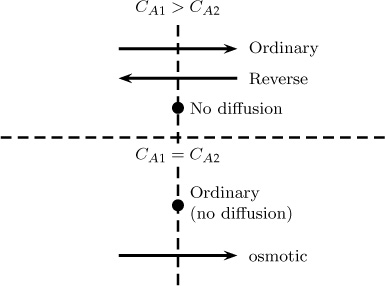
These pathological cases arise mainly when the binary pair values are vastly different—for example, in a ternary mixture of hydrogen, air, and a heavy hydrocarbon such as heptane.

Example 7.3 applies the Stefan-Maxwell equation to a binary mixture.

A second theory applicable to liquids is the hydrodynamic theory, which states that the diffusivity is proportional to the mobility of the solute. In this model, the movement of the solute is treated as a sphere moving in an infinite pool of liquid with viscosity μ_L. The frictional interpretation of diffusion discussed in Section 7.1.2 is used here. Some remarks from that section are repeated here for ease of reading.

The force needed to move a particle with a velocity of v_A (relative to B) is given, in general, by

F = fv_A

where f is the coefficient of friction and v_A is the terminal velocity of A.

For the diffusion process, the force can be identified as the negative of the gradient of the chemical potential per mole. Thus

F = –∇_μA

The model and the balance of forces on a diffusing solute are illustrated in Figure 7.6.

The balance of the forces is represented in terms of the gradient of the chemical potential as

–∇_μA = f_uA

From the flux considerations, the relative velocity of motion of A is given as:

υA=JACA=JAXxA

Hence

JA=−CxA∇μAf

The term 1/f is identified as D_A/R_gT . In turn, the preceding expression can be rearranged to

Equation 7.22 shows that the gradient of the chemical potential is more appropriately considered the driving force for mass transfer, rather than the mole fraction gradient used in the traditional Fick’s law.

For ideal systems, this expression can be shown to be the same as Fick’s law. This follows from the definition of the chemical potential. The following relation from basic thermodynamics holds:

μA=μA0+RgT InxA

Taking the derivative to get the gradient of the chemical potential, we get

Substituting in Equation 7.22, we obtain

J_A = –CD_A∇x_A

which is Fick’s law for an ideal mixture of liquids. The more general expression given by Equation 7.22 then provides an extension for diffusion in non-ideal systems. Moreover, the frictional interpretation provides a link to the molecular-level interpretation for diffusion and leads to a methodology to predict the diffusion coefficient. These two effects are explored in detail in the following sections.

where f is the frictional coefficient based on the number of moles of A. For the molecular model, it is more useful to write this relation as follows:

where f₁₂ is the force per molecule. Note that κ = R_g/N_avg has been used here to get from one form to the other.

At this point we use concepts from the fluid dynamics of slow flow, also called Stokes flow. The velocity of motion on a spherical particle in a liquid under slow flow conditions is related to the force F acting on the particle, and this relation is known as Stokes law:

where r_A is the solute radius. Hence 6πμ_Lr_A can be identified as the friction coefficient f₁₂.

Note: μ_L is the viscosity of the liquid medium (as indicated by the subscript L) and should not be confused with chemical potential.

Using the expression for f₁₂ from Stokes law (Equation 7.25), we obtain

Equation 7.27 is the Stokes-Einstein equation, which is widely used as a starting model for liquid-phase diffusivity predictions. Predictions made using Equation 7.27 are fairly accurate under the conditions used in the model derivation—namely, a small rigid sphere (solute) moving in a continuum (solvent). Hence the model is representative of experiments in which the solute radius to solvent radius ratio is smaller than 5. For solute molecules with complex structure, a correction factor is often applied and a modified equation used. Nevertheless, a key result that emerges from Equation 7.27 is that

DAμLT=constant

which fits the data for a large class of molecules. Indeed, this relation may hold even with molecules for which the Stokes-Einstein description may not be a good fit, such as nonspherical molecules and long-chain proteins.

DA=7.4×10-12(ϕMS)1/2TμLV^A0.6

where V^A is the molar volume of the solute A (in cm³/mol) and M_S is the molecular weight of the solvent (in g/mol). Also the viscosity, μ_L, is in centipoise which is equivalent to 0.001 Pa ˙ s, the S.I. unit for viscosity. The calculated value of D is given in units of m²/s here.

The empirical parameter, ø, in the preceding equation is known as the association parameter. It has a value of 1 for most organic solvents, 1.9 for methanol, 1.5 for ethanol, and 2.6 for water. Note that the equation has a form similar to that of the Stokes-Einstein equation (D_Aμ_L/T is a constant), and the dependencies of the temperature and the liquid viscosity are identical. The equation is not very accurate for concentrated systems, as the diffusion coefficient varies strongly with concentration. An activity correction is usually applied in such cases, as discussed in the Section 7.3.

The data for molar volume have been tabulated for many compounds, and some are provided in Table 7.4.

Table 7.4 Molar Volume for Some Common Species in Liquid Phase

Solute	Hydrogen	Oxygen	CO2	NH3	Water
V^s, cm3/mol	14.3	5.6	34.0	25.8	18.9

In the absence of such data, the following correlation developed by Tyn and Calus (1975) can be used:

VA=0.258Vc1.048

where V_c is the critical volume of the solute in cm³/gmol .

Group contribution methods are also available to calculate this parameter, as discussed by Le Bas (1915). In this method, atomic volume increments are added together as per the molecular formula to obtain the molecular volume. The use of Wilke-Chang equation is shown in Example 7.4.

The Wilke-Chang correlation is suitable only for dilute concentrations of the solute. One consequence is that the binary diffusivity in an A-lean system (denoted here as D_A) is not the same as the binary pair diffusivity in an A-rich system (denoted as D_B here). This is because the environment (solvent) seen in an A-lean system (full of B) is different from that in an A-rich system (full of A). The values D_A and D_B are referred to as infinite dilution values.

For concentrated solutions, the following Vignes (1966) equation is often useful:

where D_A is the diffusion coefficient of A in a B-rich mixture and D_B is the diffusion coefficient of B in an A-rich mixture, with x being the mole fraction as usual. This relation can be viewed as logarithmic averaging of the two endpoint values.

An alternative way is to take the simple linear average:

In both cases, we find the diffusion coefficient is concentration dependent.

Having discussed some predictive methods for liquid-phase diffusivity, we now look at the case of non-ideal liquid mixtures, for which where a thermodynamic correction is needed.

The chemical potential gradient can be considered to be the driving force for diffusion rather than the concentration gradients. This leads to a modified form of Fick’s law that includes a correction factor known as the activity correction. The details are shown next.

The gradient for the chemical potential can be written as

In these equations, a_A is the activity of species A in the mixture; x_A is the mole fraction as usual. Using the expression for ∇μ_A in Equation 7.22, the Fick’s law type of model takes the following form:

For an ideal solution, the term d ln a_A/d ln y_A is equal to 1; hence Fick’s law holds in the form stated earlier. For non-ideal solutions, Equation 7.32 may be written in a form analogous to Fick’s law:

where D˚_AB is the representative observed diffusion coefficient, which becomes equal to

Also a_A = γ_Ax_A, where γ_A is the activity coefficient of A. Hence

dln aAdln xA=1+(dlnγAdlnxA)

Using this definition in Equation 7.34, we find

DAB∘=DAB[1+(dlnγAdln xA)]

The term in the square brackets is called the (thermodynamic) activity correction factor.

The term D_AB on the right side of the equation is also a function of concentration, since it should be some average of the infinite solution values (see Equation 7.28 or 7.29). Using Equation 7.29 and combining it with the previous equation leads to the the Darken relation:

This relation is commonly used to interpret and model diffusion in liquids.

Note: In many design applications, these complexities are ignored and absorbed in other fitting parameters. In other words, a fitted value of diffusion coefficient is used. Nevertheless, one has to bear these considerations in mind for more accurate modeling of mass transport in liquid–liquid systems.

In general, the activity coefficient is related to the excess free energy GAE as follows:

The excess free energy is given by various models for non-ideal behavior due to differences in molar sizes, intermolecular forces, degree of hydrogen bonding, and other factors. These details are given in thermodynamic books. For binary systems, the Redlich-Kister equation is often used:

GAERgT=xAxB[A+B(xA-xB)+C(xA-xB)2]

where A, B, and C are fitted parameters.

The simplest model for γ is the obtained by keeping only the first term, which leads to the one-parameter Margules equation. This produces the following expression for the activity coefficient:

In γA=Axb2=A(1−xA)2

The model presents a symmetric variation of the activity coefficient that is rarely observed. Thus this model is not suitable for thermodynamic correction for certain ranges of A. For example, the diffusion coefficient can become negative for certain range of mole fractions if the parameter A is greater than 2.

A two-parameter model is often used in which A is replaced by a linear function of the mole fraction:

ln γ_A = (1 – x_A)²[A₁₂ + 2x_A(A₂₁ – A₁₂)]

This change is often sufficient to incorporate the effect of non-idealities on the prediction of the diffusivity. A more detailed NRTL model using three parameters may be more accurate, though. We now show the use of activity correction in Example 7.5.

D=Ro2fυω

where R_o is the spacing between atoms, f_v is the fraction of vacant sites in the crystal, and ω is the jump frequency.

Interstitial diffusion is modeled as

D = D₀ exp(–E/κT)

where E is the activation energy needed to jump to the adjacent site and D₀ is the pre-exponential factor. The activation energy is usually measured in electron-volts (eV). Hence the Boltzmann constant κ is used in the exponential term; it is equal to 8.617 × 10^–5eV/K.

Substitution diffusion is an activated process but requires a lattice vacancy to form or exist. This requires an extra activation energy, denoted as E_v. Thus substitution diffusion is modeled by including two activation parameters, E and E_v:

D = D₀ exp(–(E + E_v)/κT)

Many dopants can exist in both interstitial and substitutional sites. The diffusion can then occur by both mechanisms. Although the substitutional concentration is usually larger than the interstitial concentration, the interstitial jump is much faster than the substitutional component. Consequently, the overall diffusion is often governed by interstitial concentration.

Concentration-dependent diffusion is often observed with dopants in silicon. A power law type of model is commonly used for these cases. More details are given by Ghandhi (1983) and Middleman (1993). The mechanisms can be complex, and these sources should be consulted for more details. A few examples are given here to give a feel for the values of diffusion of some dopants in silicon.

Boron in Silicon: The data at concentrations of boron less than 10¹⁹ atoms/cm³ are correlated by an Arrhenius type of model:

D=3.17exp(-3.59κT)

where κ = 8.62 × 10^–5 eV/K. Note that the activation energy is usually reported in electron-volts in these systems, whereas the diffusivity is in cm²/s. For higher concentrations, diffusivity is a linear function of boron concentration.

Arsenic in Silicon: The arsenic diffusion follows a similar pattern with the following values:

D=23exp(-4.1κT)

Phosphorus in Silicon: Phosphorus diffusion follows a similar pattern, with the diffusion coefficient remaining constant at low concentrations. It then decreases with concentration first and subsequently increases at larger concentration levels.

Note: Diffusion of phosphorus induces an electric field, and the combined mechanism should consider the effect of migration due to the electric field. Details are given in the paper by Fair and Tsai (1997) and in some other sources (Middleman and Hochberg, 1993).

The criterion used to distinguish between the two mechanisms is comparison of the pore diameter, d_p, to the mean free path of the gas molecules, λ. If d_p << λ, the Knudsen diffusion is the main mode of diffusion. The diffusion coefficient for this case is modeled using concepts similar to those found in the kinetic theory of gases:

Here c¯ is the mean molecular velocity given earlier in Equation 7.3. The only difference between this equation and that from kinetic theory is that the mean free path λ is not used, but instead is replaced by d_p, the pore diameter.

Using the expression for the mean velocity from kinetic theory and substituting some universal constants, we can derive the following equation from Equation 7.37 for the Kundsen diffusion coefficient:

The units are cm for d_p g/mol for M_A, and cm²/s for D.

A combined model is used for the overall diffusion:

where D_K is the Knudsen diffusion coefficient (Equation 7.38) and D_AB is the gas-phase (binary pair) diffusivity. For small pores, the first term on the right side of Equation 7.39 dominates, so the overall diffusion coefficient depends on the pore diameter. For large pores, the second term dominates, so the diffusion coefficient is not a function of the pore diameter. Example 7.6 provides an example of the calculation of diffusivity in a single pore.

For liquid pores, there is no Kundsen diffusion since the mechanism of diffusion is not collision, but rather frictional flow. Nevertheless, liquid-filled pores of a small size exhibit the phenomenon known as hindered diffusion, which is discussed in the following section.

A schematic of a small molecule diffusing in a small pore is shown in Figure 7.10.

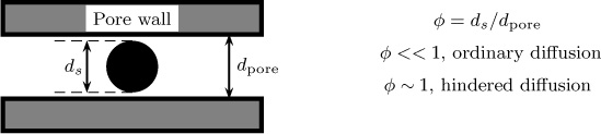
The ratio of the solute diameter to the pore diameter is denoted by φ. The hindered diffusion becomes important if φ is close to 1 and is often modeled by introducing two correction factors, F₁ and F₂, that depend on φ. The first correction factor is simply a geometric factor known as the steric partition constant and is defined as follows:

F₁(φ) = (1 – φ)²

The second correction factor is known as the hydrodynamic hindrance factor:

F₂(φ) = 1 – 2.104φ + 2.09φ³ – 0.95φ⁵

The diffusion coefficient in small pores is obtained by multiplying the large pore value by F₁F₂. This is known as the Renken (1954) correction.

Hindered transport has been reviewed by Deen (1992). This paper is a useful reading for students who wish to explore this field further.

Adsorbed species can also move along the surface of the pore walls. This phenomenon, known as surface diffusion, and may operate in parallel with the pore diffusion.

A simple model is to define an effective diffusivity with the following equation:

D_e = D_pore∊_p/τ

where ∊_p is the catalyst (particle) porosity and τ is a tortuosity factor. The factor ∊_p accounts for the reduced area for diffusion, while the factor τ is the correction for non-straight pores. These factors depend on the pore structure. Two common models for pore structure are shown in Figure 7.11. The first model assumes pores are composed of capillaries of various sizes connected in a random manner. The second model is applicable when the catalyst is formed by compaction of small, nonporous grains to form a porous pellet.

The pore diameter is often calculated by the following relation:

dp=4ϵpSp

where ∊_p is the particle porosity and S_p is the surface area of the pores per unit volume. The basis for this equation is the hydraulic radius concept, which is widely used in fluid mechanics for studying flow in noncircular channels. This concept applies to materials in which the pores show a unimodal distribution.

Example 7.7 shows some calculations for these quantities.

The tortuosity factor is in the range of 2 to 3 for many catalysts with unimodel pore size distribution. Wakao and Smith (1964) suggest a value of 1/∊_p could be used as an approximation in the absence of experimental measurements. Carniglia (1986) suggested the following equation for tortuosity:

τ=(2.23-1.13υpρB)(0.924Sp∑Δυpdp)1+α

where v_p is the total pore volume, Δv_p is the pore volume within an interval with an average pore diameter of d_p, S_p is the BET surface area, and α is an exponent that depends on the pore shape. To use this equation, information is needed regarding the pore size distribution, which can be obtained from mercury porosimetry.

The following equation can be derived based on this concept; it is shown directly without derivation here:

De=ϵm2Dm+ϵμ21+3ϵm1−ϵmDμ

The pore scale diffusivity D_m and D_μ are estimated by the single-pore consideration given by Equation 7.39. This requires an average diameter for the macropores and micropores. These diameters reflect the surface area of the macropores and micropores. Note that Kundsen diffusion may be the controlling mechanism in micropore transport, whereas bulk diffusion may dominate the transport in macropores. Hence the pore-scale diffusivity values must be computed separately for the micropores and the macropores.

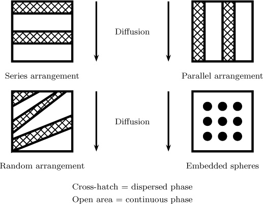
Consider a material made of two types of matrices, with permeability P_c and P_d, respectively. Let ∊_d be the volume fraction made of material d; 1 – ∊_d is then the volume fraction of the second material. An effective permeability of the material P_e is to be computed. Here we discuss first two simple models: parallel and series arrangement of the laminate series. They provide two limiting cases to the general case (Figure 7.13).

For a series arrangement, the following equation—which is based on adding resistances in series—is used:

1Pe=1−ϵdPc+ϵdPd

This can be rearranged to

Pe=PcPdPd(1-ϵd)+Pcϵd

The equation for the calculation of the permeability of parallel arrangement of laminates is

P_e = P_c(1 – ∊_d) + P_d∊_d

The predictions of the parallel and series modes bound the expected behavior of the composite matrix. Students studying heat transfer will be able to relate this to conduction in series versus in parallel.

An equation for the general case (in which the two materials are distributed in a random manner) was derived by Petropoulos (1985):

Pe=Pc[nPd+(1-n)Pc-(1-n)ϵd(Pc-Pd)nPd+(1-n)Pc+nϵd(Pc-Pd]

Here n is the shape parameter of the dispersed phase. The parallel arrangement corresponds to n = 0, a series arrangement to n = 1, and an embedded sphere (shown next) to n = 1/3.

In another useful model, one of the phases, denoted as d or the dispersed phase, is embedded in the matrix as solid spheres in a second phase, the continuous phase. The permeability of this composite can be calculated using an equation originally derived by Maxwell in 1873 in the context of electromagnetism to describe a composite dielectric medium:

Pe=Pc[Pd+2Pc-2ϵd(Pc-Pd)Pd+2Pc+ϵd(Pc-Pd]

A special case occurs when P_d is zero; it is applicable to the effective diffusivity in gas pores of a porous catalyst. In this special case:

De=Dcϵc3-ϵc

Compare this relation with the expression for the effective diffusivity. The preceding equation predicts that the tortuosity factor is 3 – ∊_c, which gives credence to the values of 2 to 3 for the tortuosity factor used in the reaction engineering literature.

In such gas separation processes, we require both a high rate of diffusion and selectivity for a particular gas. Solute (water) diffusion in polymeric food wrapping is an important application of this process, in which we need the polymer to act as a barrier. Transport of ions in a conducting polymeric matrix is important in electrochemistry. Oxygen permeability coefficients in polymers used to make hard and soft contact lenses are an important biomedical application, as is diffusion of drugs across a swollen polymeric capsule.

The glass transition temperature is an important parameter affecting the rate of diffusion. This is the temperature at which the polymer changes from a brittle solid structure to a glassy rubbery structure. If the glass transition temperature is exceeded, the diffusivity may change by an order of magnitude. Size of the permeate is an important factor as well. Swelling is another factor, as swelling typically increases the diffusion coefficient.

Recall that permeability is a product of diffusivity and solubility. Diffusivity increases with temperature, whereas solubility decreases under the same condition. The combined effect is that the permeability often shows a maximum with temperature.

Free volume theory is often used as a platform to predict diffusion. A free volume is a space that the solute molecule can occupy, similar to the holes observed in liquid diffusion. The free volume increases with an increase in temperature. The temperature at which the free volume increases rapidly is the glass transition temperature.

Neogi (1996) and Peppas and Meadows (1983) are good starting references that provide an introduction to the various theories that apply to polymeric membranes. These theories should be interpreted as a fitting tool rather than a complete predictive tool, since this research remains in its infancy. Many parameters can be adjusted to fit the data; however, the theoretical underpinnings in these models provide a solid platform for future development in this area. More coupling with molecular-level models can be expected in this field. The discussion provided in this section is rather brief and intended to give just an overview of this topic.

• Dissociation Effects: Dissociation effects are of importance in liquid–liquid systems where a solute associates with the solvent molecules and the associated pair diffuses together. The solute may associate with itself (a type of dimer) and the diffusion may be controlled by that of the dimer rather than the original solute. Also the solute may dissociate and the two ions formed may then diffuse as a pair together with the diffusion of any undissociated solute. Diffusion of acetic acid in water is an example:

  CH₃COOH ⇌ CH₃COO^– + H⁺

  The diffusion rate of acetic acid is therefore determined by the diffusion of the undissociated species CH₃COOH and the diffusion of the ions, CH₃COO^–, and H⁺. Strong and complicated dependency on the concentration and the pH of the solution can be expected in many of these cases (since pH changes the extent of dissociation).

• Facilitated Diffusion: Facilitated diffusion is a complexity usually associated with transport in membranes where a simultaneous chemical reaction is also taking place. A chemical reaction binds the diffusing species and enhances its transport. Life itself would not exist but for oxygen–hemoglobin interactions that proceed by facilitated diffusion. Similarly, many membranes (especially biological) have carriers, and the diffusing species binds to the carrier. Both the species and the carrier diffuse across the membrane , such that the transport is considered “facilitated.” This topic is studied in further detail in Chapter 22.

• Active Diffusion: Active transport refers to diffusion against a concentration gradient at the expense of some work done on the system. A common example is the Na⁺-K⁺ pump, which is common across all living systems. This “pump” involves transport of sodium ions against a concentration gradient using the hydrolysis of ATP (adenosine triphosphate) as the energy source. The free energy released in the hydrolysis is used to overcome the difference in chemical potential of Na⁺, and a concentration difference on the order of 110 mol/m³ may exist for the steady state conditions across a cell membrane.

• Thermal Diffusion: In thermal diffusion, a species diffuses due to the presence of a temperature effect. The additional mass flux resulting from thermal diffusion is usually modeled as

  JA, Thermal diffusion=−CDABkT∇In T(7.40)

  where k_T is the thermal diffusion factor. In general for binary systems, species with larger weight move to the colder region, and vice versa.

• Pressure Diffusion: In pressure diffusion, a species diffuses as a result of a pressure gradient. The contribution of pressure to diffusion is modeled as

  JA, Pressure diffusion=−DAByARgT(1−MAM¯)∇P(7.41)

• Diffusion of Charged Species: Diffusion of charged species (e.g., ions) is important in systems such as electrochemical processes and fuel cells. The transport rate is augmented by adding the electrochemical potential as an additional driving force. Simultaneous solution of the diffusion equation and the electric field is needed for such problems. Chapter 16 provides a more detailed discussion of this subject.

7.2 How does the mean free path change with temperature and pressure?

7.3 How does the average speed of random molecular motion change with temperature and pressure?

7.4 What are the effects of temperature and pressure on binary diffusivity in a gas mixture?

7.5 Verify the dimensional consistency of Equation 7.6.

7.6 What is the effect of temperature on the diffusivity of a solute in a liquid?

7.7 Why and when is a thermodynamic correction needed to calculate the diffusion coefficient?

7.8 What is the Vignes relation?

7.9 What is the Darken equation and when is it used?

7.10 Can the parameter A be negative in the one-parameter Margules equation? If so, for which case?

7.11 What is Knudsen diffusion? When is it important?

7.12 What is the effect of temperature on the Knudsen diffusion coefficient? How does it compare to bulk (gas–gas) diffusion?

7.13 When does a pressure gradient build up in a porous solid?

7.14 What is hindered diffusion? When is it important?

7.15 What are the two factors to correct for hindered diffusion of a solute in a liquid-filled pore?

7.16 What is meant by the tortousity factor? State a simple formula to calculate this factor that can be used in the absence of experimental data.

7.17 How is the effective diffusion in a catalyst with a bimodal pore distribution calculated?

7.18 What is the glass transition temperature, and how does it affect diffusion in a polymer?

7.19 What is the effect of temperature on the diffusion coefficient of a gas in a polymeric solid?

7.20 What is facilitated diffusion?

7.21 What are thermal diffusion and pressure diffusion?

f(c)=4πα3/2c2 exp(−αc2)

where α = m/(2κT).

Plot the function for CO₂ at 300 K. Show that the area under the distribution function is unity, as would be expected for any probability distribution function.

Find the mean speed, defined as

c¯=∫0∞cf(c)dc

7.2 Kinetic theory parameters for an oxygen molecule. Calculate the mass of an oxygen molecule and the average speed of the molecules c¯ are based on kinetic theory at a temperature of 273 K and 1 atm pressure. Compare this speed to the speed of sound in the medium. Compare this speed to the speed of Superman. Hint: Superman can reach the top of the St. Louis Arch 2.5 seconds. Also calculate the mean free path, assuming a molecular diameter of 3 ^°A (0.3 nm). Determine the self-diffusion coefficient of oxygen. Compare it with the oxygen–air binary diffusivity value of 1.75 × 10^–5 m²/s.

7.3 Mean free path and mean speed. Calculate the mean free path of a nitrogen molecule at 1 atm, at a low vacuum (1000 Pa), and at a high vacuum (100 Pa). Assume a molecular diameter of 0.3 nm. The molecular Knudsden number is defined that a dimensionless number defined as the ratio of the molecular mean free path length to the molecular diameter. Find its value for nitrogen. Also calculate the mean molecular speed at 1 atm and a temperature of 300 K. How does it compare with the speed of sound?

7.4 Lennard-Jones parameter from critical properties. The critical temperature for CO₂ is 304.25 K and the critical pressure is 7.35 MPa. Estimate the σ and ∊ parameters and compare them with the values given in Table 7.1.

7.5 Binary pair diffusivity in the gas phase. Estimate the diffusion coefficient of CO₂ in air at 20° C and 1 atm pressure using the Chapman-Enskog equation. Compare the results using the Fuller correlation.

7.6 Stefan-Maxwell equation for a ternary gas mixture. Write out in detail the Stefan-Maxwell equation for a gas A diffusing in a mixture of B and C. Now consider the case in which only species A has a net non-zero combined flux— In other words, N_B and N_C are zero. Simplify the Stefan-Maxwll model for this case. Compare the result with the Wilke equation for a pseudo-binary diffusivity.

7.7 Liquid-phase diffusivity of a dissolved gas. Calculate the diffusion coefficient of dissolved CO₂ in water at 300 K.

7.8 Liquid-phase diffusivity in infinite dilution conditions. Calculate the diffusion coefficient of ethanol in water (dilute solution with a large mole fraction of water) at 298 K. using the molar volume based on the density and the molar volume based on the group contribution method. The atomic increments are carbon = 14.8, hydrogen = 3.7, and oxygen = 7.4 (all in cm³/mol), as reported in Le Bas. Also calculate the diffusivity of water in ethanol (dilute solution with a large mole fraction of ethanol).

7.9 Liquid-phase diffusivity as a function of composition. Calculate and plot the diffusivity as a function of the mole fraction for an ethanol–water mixture using either the linear interpolation or the Vignes equation. Ignore the thermodynamic correction. Now find the activity coefficient of ethanol as a function of composition using thermodynamic data and correct the results for the diffusivity using the thermodynamic correction factor.

7.10 Diffusivity in an acetone–water mixture. Verify the calculations for the diffusion coefficient of acetone in water for a 50 mole % mixture, as shown in Example 7.5. Now find the values at various compositions and plot the diffusivity as a function of mole fraction of acetone.

7.11 One-parameter model for activity coefficient. Consider the simplest model for the activity coefficient:

In γA=AxB2=A(1−xA)2

Calculate γ_A and plot it as a function of the mole fraction of A for different values of A (A = 0, which is the ideal case; A = 1; A = 2 and 3). The correction becomes negative for certain value of A, which means the observed diffusion coefficient becomes negative! Provide an explanation for this outcome.

7.12 Use of Gibbs-Duhem equation. State the Gibbs-Duhem equation. Using this equation, show that the thermodynamic correction for diffusivity for species A is the same as that for B in a binary mixture. In other words, verify that the sum of the diffusion fluxes is zero at any specified mole fraction value. Also verify that D_AB = D_BA at a fixed concentration, although the values may be concentration dependent.

7.13 Diffusion in a straight pore. Calculate the value for silane diffusing in a 10-μm cylindrical pore at 900 K, which is representative of the deposition of solid silicon in thin tubes. Determine the dominant mechanism for diffusion in this case.

7.14 Hindered diffusion in a nanosized pore. Glucose is diffusing across a microporous membrane with pores of 2-nm diameter. The mean diameter of the glucose molecule is about 0.86 nm. Temperature is 300 K. Find the diffusion coefficient using the Stokes-Einstein equation. To what extent is the hindered diffusion correction important in this case?

7.15 Size exclusion–based separation. A protein solution is separated from water by allowing it to diffuse across a porous nanosize membrane. The size of the protein is 25 nm. Find the diameter of the membrane to have a steric partition coefficient of 0.64. If a second protein has a a size of 50 nm, find the relative exclusion of this protein in the membrane.

7.16 Effective diffusivity in a porous catalyst. Calculate the effective diffusivity of ethylene diffusing in hydrogen gas at 1 atm pressure at a temperature of 298 K given the following properties of the catalyst: porosity = 0.4; surface area = 100 m²/g; bulk density of the catalyst = 1.4 g/cm³.

7.17 Bimodal pore distribution. A porous catalyst has a bimodal distribution with porosity of 0.233 in the micropores and 0.492 in the macropores. The average pore radii values are 40 nm in the micropores and 2 μm in the macropores. Find the effective diffusivity for a methane–air mixture.

7.18 Diffusion in a composite matrix. A polymeric membrane is made of two material with permeability of 1 × 10^–5 and 4 × 10^–5, respectively. The second material is embedded in the first, with a distribution of 15%. Calculate the overall permeability assuming (a) a series arrangement, (b) a parallel arrangement, and (c) the second material embedded as small spheres in the first material.