
Chapter 19. Reacting Solids
Learning Objectives
After completing this chapter, you will be able to:
Show how mass transfer affects the rate at which a gas reacts with a solid.
Calculate the rate of reaction in a relatively non-porous solid based on the so-called shrinking core model.
Calculate the rate of reaction of a porous solid on the basis of a diffusion-reaction model.
Derive expressions for the conversion of the solid as a function of time.
Characterize the structural changes of the solid due to a reaction and see how it affects transport properties and the rate of conversion of the solid.
Examine the effects of structural changes such as pore plugging/ opening and in some cases, an incomplete conversion of the solid reactant.
Examine diffusional effects in solid–solid reactions.
Reactions where a solid reacts with a gas are very common in chemical, metallurgical, environmental, and electronic processes. Combustion of a coal particle is an example in the energy production sector as well as the process of gasification of coal where coal is reacted with steam to produce a mixture of CO and H2 (syngas). In metallurgical industries, the reduction of metal ores (e.g., NiO) with hydrogen to produce metals (e.g., Ni) is an important application where a gas–solid reaction is encountered. Direct reduction of iron ores with hydrogen is another example. Oxidation of silicon to form an insulating film is an important application in the semiconductor fabrication of MOS (metal oxide semiconductor) devices. Similarly, in the production of polysilicon for solar cells, the precursor production involves many steps of gas–solid reactions such as chlorination of silicon, the deposition reaction of silane on a solid substrate, hydro-chlorination of silicon, and so on. In the pollution treatment field, CO2 removal is an important problem and CO2 capture by reaction with calcined lime (CaO) is an example of reacting solids.
In all these cases and other similar processes mass transfer effects play an important role as these are heterogeneous systems. Thus external (gas film) diffusion and pore diffusion in the interior of the solid affect the rate at which the solids react at the gas–solid interface. The scope of this chapter is therefore to study mass transfer effects in these systems.
The starting reacting solid can be relatively non-porous or highly porous and the modeling of the systems for these cases takes different approaches. For non-porous systems the reaction occurs at a sharp gas–solid interface. External or film mass transfer followed by diffusion through the product layer (in some cases) and the surface reaction are the factors to be considered. Analysis of such systems is discussed first.
For porous systems, the reaction occurs on the interior surface of the solid and hence simultaneous reaction during pore diffusion plays a role. The mass transfer steps here are similar to those for a porous catalyst analyzed in Chapter 18. However, an important difference is that the solid properties change as the solids react. This changes the porosity and in turn the effective diffusivity in the solid. We consider the various ways to represent how the pore structure affects the rate of reaction.
Diffusional effects in scenarios of a solid reacting with a second solid are also briefly discussed.
19.1 Shrinking Core Model
The reaction scheme considered is that of a gaseous reactant A reacting with a solid B in the following reaction scheme:
A+ νBB → Products
One widely used model for this reaction is the shrinking core model. This model can be applied to the case where there is no solid product and also to a case where there is solid product formed. The analyses for the two cases are slightly different and therefore treated separately in the following subsections. In both cases the solid reactant B is assumed to be non-porous so that the reaction occurs at a sharp interface.
19.1.1 No Solid Product
Figure 19.1 illustrates the transport steps leading to the reaction. The reaction is assumed to follow two steps: external diffusion of the gaseous reactant, A, through the gas film from bulk gas to the surface of the solid followed by a reaction at the solid surface. The combination of these two steps leads to an overall rate constant, which is discussed next.

Figure 19.1 Schematic of a solid reacting to form a gaseous product. Note: The gas film thickness is exaggerated.
Overall Rate Constant
The pseudo-steady state model is used for the gaseous transport and reaction, which is then coupled with the transient macroscopic model used for the solid. The modeling goal is to see the rate at which the solids reacts and to examine the effect of operating parameters on the rate:
Rate of mass transfer from gas to the surface = km(CAb – CAs)
This is balanced by the surface reaction assuming a pseudo-steady state:
Rate of reaction per unit surface area of the solid = ksCAs
A first-order surface reaction is considered here. The two rates are equal due to the pseudo-steady state assumption and hence CAs can be eliminated and a rate expression based on bulk gas concentration can be derived.
This rate equation combining the two transport effects in turn leads to an apparent or overall rate constant, which is defined as
Rate per unit area of B = k0CAb
This overall rate constant can be shown to be
Note that this can also be expressed as k0 = kskm/(ks + km). Also note that depending on the relative values of the mass transfer coefficient and the surface reaction constant two limiting steps can be identified:
The process can be mass transfer limiting if km << ks and in this case k0 = km.
The chemical kinetics can be rate limiting if ks << km and in this case k0 = ks.
The rate of reaction can now be incorporated into the transient mass balance for the solid to study the conversion of the solid as a function of time, which is presented next. It is useful to note that this part of the model is similar to the model for sublimation of a solid considered in Section 3.2.
Solid Reactant Mass Balance
The rate of shrinkage of the particles (assuming a spherical shape) is calculated by writing a mass balance for the solid phase reactant:
where νB is the stoichiometric coefficient of B and CB0 is the concentration of solid B, which is equal to solid density divided by the molecular weight of B, that is, ρB/MB. The previous equation can be simplified to
The variables can be separated and the solution for time needed to reach a particular radius R(t) can be formally written as
Here we have also used Equation 19.1 for k0 in terms of ks and km. We also note that km depends on R and hence the explicit dependency of this term on R is also noted in the second integral on the right-hand side. The two integrals on the right-hand side can be written separately and the time needed for the solid to shrink to any R is given as
where tR is the first term on the right-hand side of Equation 19.2:
and tM is the second term:
The first term on the right-hand side can be integrated directly since ks is not a function of the radius. The result is usually expressed in terms of the conversion of the solid B, denoted as XB. This is related to R as
Hence the integrated form of the Equation 19.4 is
In order to integrate the second term in Equation 19.2 the functional dependency of km on R should be taken into account. In accordance with the Ranz-Marshall equation shown in Chapter 3, the dependency of mass transfer coefficient on particle radius is as follows:
For small particles and/or small gas velocity km ∝ R–1.
For large particles and/or large external gas flow rates km ∝ R–0.5.
Hence the radius dependency may change with time. At the start if we have large particles the dependency is –0.5 and will keep changing with time as the solid radius keeps decreasing; it may switch to the small particle regime where the dependency is –1.
Consider the case for small particles with low gas flow; here the mass transfer coefficient is given as
Hence the integrated form of Equaton 19.5 is
If ks << km right from the beginning, the process is under a kinetic regime and the film mass transfer resistance need not be accounted for.
A few remarks on the kinetics and mechanism of solid–gas reactions may be in order:
The order of the reaction with respect to the solid concentration is often a fitted parameter rather than that result due to mechanistic considerations. This is unlike gas–gas reactions. The effect of concentration of a solid cannot be easily studied unlike a gaseous system since the activity of the solid reactant is one.
The surface reaction can proceed in two ways. The first is an adsorption + surface reaction mechanism. Gas first adsorbs on the surface and the adsorbed species then reacts with B on the surface of the solid. Models similar to gas–solid catalytic reactions, that is, Langmuir-Hinshelwood type of models, have been proposed for these cases. The second is the direct attack of gas on individual sites of a solid that are the most reactive (active sites). Crystal defects and orientation of the surface will have a strong effect in this case.
In some cases the reaction may proceed at only some preferential directions on the solid surface, the so called wormhole effect. Modeling and analysis of wormhole formation in reactive dissolution of carbonate rocks has been studied by Kalia and Balakotaiah (2007, 2009) and Fredd and Fogler (1998) and other references cited within these sources.
19.1.2 Solid Product: Ash Layer Effects
If the product is a solid it forms a layer near the external surface of the solid. This is known as the ash layer. The layer is assumed to be porous and a diffusion from the surface through the ash layer needs to be considered as an additional resistance.
The concentration profiles when the product layer forms are shown in Figure 19.2. The ash layer is assumed to occupy the region from λ to R at any instant of time. The reaction plane is now located at λ, which moves inward with time.

Figure 19.2 Representation of steps in reaction of a non-porous solid B with a gas leading to a solid product. The solid product is called the “ash” layer.
The pseudo-steady state assumption is made for the solid. Let λ be the position of the ash layer at any instant of time as shown in Figure 19.2.
The reaction takes place due to three steps in series, noted in the following together with the corresponding resistance.
The first step is the gas film diffusion; the mole/s transported are given as
The resistance for this step is 1/(4πR2km).
The second step is ash layer diffusion with the following rate:
The resistance is (R – λ)/(4πR DeA).
Finally the surface reaction takes place at a sharp interface located at λ:
The resistance is 1/(4πλ2ks).
The overall resistance is the sum of these resistances, and the rate at which the gaseous species is consumed by reaction is
Here k0 is the overall rate constant, defined as
The three terms on the right-hand side are due to the three resistances indicated earlier. The dimensionless location of reaction plane λ*, defined as λ/R, is used for the convenience of later algebra.
Now we are in position to calculate the rate at which the solid phase reactant is consumed by writing a transient mass balance for the solid reactant. The method is similar to the solid balance discussed in the previous section and therefore not shown in detail. The following equation can be derived for the change in the reaction plane location with time:
Using Equation 19.12 for k0 and separating the variables the result for the time needed to achieve a given conversion can be expressed as a sum of three terms, each corresponding to one of the resistances:
Here tm is the contribution of the mass transfer resistance:
Note that the external mass transfer coefficient does not change as a function of time now since the overall radius of the particle remains constant. Particle size may change slightly due to shrinkage or expansion, which can be accounted for by a volume balance. These details are not addressed here.
The tD term in Equation 19.14 is the time needed if ash layer resistance were in control:
Finally tR term is the time if the reaction were in control:
The final results are presented in terms of the conversion of the solid, defined as
XB = 1 – (λ*)3
Students may wish to verify the following results for the three contributions to the total time needed to achieve a given conversion.
The following diagnostic criteria given by Levenspiel (1999) are useful for finding the controlling regime:
The time for complete conversion is proportional to R2 if ash diffusion is controlling.
The time for complete conversion is proportional to R if surface reaction is controlling.
The time for complete conversion is proportional to Rn where n is between 1.5 to 2.0 if external mass transfer is controlling. This is because km is a function of the radius. In this case the conversion should also change if gas velocity is changed.
Hence experiments with particles of different initial solid radius are indicative of the prevailing control regime for the given experimental conditions. Note that the controlling regime may change during the course of the reaction. Thus in the initial stages the process may be reaction controlled since there is no significant ash layer. In the later stages the process may be ash diffusion controlled. These changes are not captured in the above simple criteria and parameter fitting with tools available in MATLAB or other similar softwares may have to be used.
19.2 Volume Reaction Model
Volume reaction models apply when the particle porosity is large. Since the solid now contains a significant amount of pores, the gas can diffuse into the interior of the pellet and react over the interior surface of the pore rather than at a sharp interface. The schematic mechanism is shown in Figure 19.3, where we show a representative pore located between any differential control volume between r and r + Δr.

The gas diffuses into the pores, is adsorbed on the reactant surface, and reacts with B at the surface. The adsorption and reaction are lumped together and a “pseudo-homogeneous” rate of reaction is defined on the volume of the solid+gas locally at any location r. Note that a product layer can form on the surface of the solid. This layer is assumed to porous and the resistance due to the gas diffusion through this product layer is usually neglected at the first go at modeling. More detailed models account for this effect (see for example Christman and Edgar, 1983). Also the pore size changes due to product formation, which in turn affects the internal diffisivity.
19.2.1 Kinetic Model
The local rate of production of A by reaction is modeled as a power law kinetics:
where n and m are the order of reaction with respect to A and B respectively. Here CB is the local concentration of the solid reactant. The rate is defined as moles produced per unit total volume (pore + solid) per unit time.
The following remarks on the kinetic model shown above are useful:
Note the negative sign for RA since A is consumed rather than produced by reaction.
The rates are often based on the mass of the solid RA, m in which case the units will be in mol/kg sec rather than mol/m3 s. If so, we should multiply this by ρs to get RA, the volume-based rate of reaction used previously.
Rate can also be defined using the surface area of the solid, in which case the initial surface area per unit volume of the solid must be known.
The order of reaction with respect to the solid reactant is often a fitted parameter rather than a mechanism-based value. Usually it has a value ranging from 0 to 1.
The reactions often follow a two-step scheme with adsorption of A on the solid first followed by reaction with B at the surface. This is often modeled by a Langmuir kinetics of the following form:
19.2.2 Concentration Profile for Gas and Solid
A concentration profile develops for the gas similar to that for a catalytic reaction. This profile can be calculated by a diffusion-reaction model for the gaseous reactant:
where ∊p is the internal pore volume of the solid.
The diffusion coefficient is assumed to be a constant for further discussion. This parameter may change in time due to a change in the pore structure and due to reaction of solid B. Variable diffusivity analysis is briefly presented in the Section 19.3.1.
The corresponding rate of reaction of B is then incorporated into a transient mass balance for B (over a differential volume) and provides an equation to calculate the B versus t profile at each radial location:
The concentration of B is defined based on the total volume of the pellet (pore + solid) and hence the solid holdup term does not appear on the left-hand side. The RA is assumed to be given by a power law model: . Observed features of the solution for reaction, which is first order in B (m = 1) is shown next followed by a zero-order reaction (m = 0).
19.2.3 First-Order Reaction in B
In this section a first-order reaction with respect to the solid and gas is considered. Dimensionless formulation and some illustrative results are presented. The following dimensionless concentration variables are used: cA = CA/CAb and cB = CB/CBi. Here CBi is the initial concentration of the solid. Distance is scaled using the radius of the solid as ξ = r/R. Time is scaled as
τ = (νkCAb)t
This provides the following dimensionless equations to be solved for the gas phase and the solid phase:
and
Two parameters that arise in the dimensionless formulation are
This is a Thiele modulus parameter based on the initial concentration of B and
This is a capacity term representing the ratio of the reaction time constant to the time constant for internal diffusion.
The pseudo-steady state hypothesis is often used. The term containing κ in Equation 19.20 is then dropped. This is usually a good assumption for gas– solid systems since CAb is usually much smaller than CBi. Hence the accumulation in the pore phase is often small and this term can be dropped. The assumption may not be valid for liquid–solid reaction. For further discussion, we use the pseudo-steady state hypothesis.
An illustrative plot of the concentration profile of gas A and solid B within the pellet is shown in Figure 19.4.
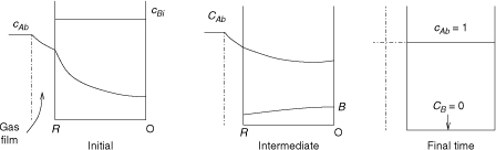
Figure 19.4 Schematic of the concentration profiles for gas A and reactant B for a (1,1) order reaction. The profile of gas A depends on the Thiele modulus and can be nearly flat (low Thiele) or very steep (large Thiele): an intermediate case is shown.
The following discussion is useful to understand the qualitative features of the volume reaction model and to identify the regime of operation. Two cases are normally distinguished: low Thiele and high Thiele. For low values of the Thiele parameter the concentration profile of A is nearly uniform in the pellet. The reaction of the solid takes place uniformly all over the pellet. This is often referred to as a homogeneous reaction model or uniform reaction model.
Uniform Reaction Model
If the Thiele modulus is small, the change in concentration of A in the solid is small. All of the solid is exposed to a nearly uniform concentration. The dimensionless concentration of A, cA, may be approximated as one here leading to a case where the reaction occurs at a constant rate throughout the pellet:
where τ is the dimensionless time.
Intermediate Range of ϕ
For intermediate Thiele modulus values there is a moderate drop in concentration as shown in Figure 19.4. The reaction of B takes place all over the pellet with the interior reacting somewhat slowly due to less availability of A due to diffusion limitation. The concentration drop gets smaller as time progresses for A and the concentration of A increases. The final concentration is unity in dimensionless units. The concentration of B drops with time. The extent of the reaction of B near the surface is larger than at the center at the beginning of the process and the concentration variation of B tends to become more uniform with the progress of time.
Large Thiele Case
For large Thiele modulus values a steep profile develops in the solid. Here a (nearly) gas depleted zone develops near the center and the reaction is confined to a zone near the surface. This zone moves inward with time. Since the reaction is first order with respect B, the concentration of B can never become negative, although it can take infinitesimally small values. Hence there is no mathematical need to consider a separate ash layer formation, unlike the case of a zero-order reaction, which is discussed in the next subsection.
An illustrative result for a (1,1) order reaction simulated numerically using the a modified MATLAB PDEPE solver is shown in Figure 19.5. The time required for a given conversion is smaller if the Thiele modulus is small and the uniform reaction model holds.
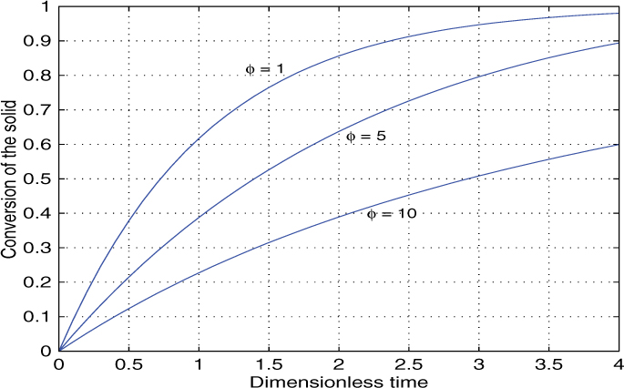
An approximate analytical solution can be obtained using the concept of cumulative concentration; this is presented as an exercise problem.
19.2.4 Zero-Order Reaction
Reactions that are zero order can exhibit an ash layer formation and hence they are treated somewhat differently compared to a first-order reaction. The concentration of B can become zero near the surface and hence it is necessary to distinguish two regions. The corrsponding concentration profiles are shown in Figure 19.6.

Figure 19.6 Schematic of the concentration profiles for gas A and reactant B for a (1,0) order reaction. An ash layer develops after the initial stage and the reaction zone moves inward with time.
In the initial stage the concentration of B is above zero everywhere. The model equations for the gas and the solid are
and
The gas concentration can be solved independently since the reaction is first order. An effectiveness factor for the drop in gas concentration is used in the solid balance. Upon integration this yields the following expression for the conversion of the solid as a function of time:
This solution is valid until the concentration of B remains finite at the surface.
In the later stages of the reaction a B depleted layer develops near the surface of the solid. The concentration of B becomes zero at a dimensionless location λ in the solid and the reaction can now take place only in the region from 0 to λ. The previous model equations now need a minor modification. Equation 19.25 has to be solved separately for the region of no B, which is from λ to 1. The rate term is set to zero in this region. The reaction zone is from λ to 0 and the rate term is retained for this region. Matching of the concentration and the flux of A on either side of λ has to be used as additional conditions. The solution for the concentration profile and the conversion of the solid with this modified model is not very complicated, but the details are not shown here. The following solution for conversion can be derived for this stage of the reaction:
where λ is given by the following equation:
The reaction zone thickness depends on the Thiele parameter. It is on the order of 0.039 for ϕ = 100. Thus the sharp interface model can be used as an approximation for such cases. Note that the sharp interface model can be viewed as a limiting case of the volume reaction model for large Thiele modulus values. Details leading to Equation 19.29 are shown in the paper by Ishida and Wen (1968).
19.3 Other Models for Gas–Solid Reactions
In this section, we briefly consider some other related models proposed for gas–solid reactions. These models incorporate additional details such as pore volume change due to a reaction and non-uniform distribution of pores in the solid. The discussion is qualitative and for more details the references cited should be consulted. First we consider the modifications to the volume reaction model to account for structural changes.
19.3.1 Effect of Structural Changes
The product formation can lead to a change in the volume of the pore and the associated changes in the diffusion coefficient. The extent of this change depends on the nature of the product formed and the relative volume the product occupies relative to the solid reactant B. A relative molar volume ratio parameter is defined:
This parameter is a measure of the ratio of the volume of product formed per unit volume of the reactant. If ZV less than one, the pore volume increases, while the pore volume decreases if ZV is greater than one.
The porosity variation can then be modeled as
Correspondingly the diffusion coefficient is assumed to vary as
where n has a range of values from between 2 and 3 depending on the porosity and tortuosity of the solid. A value of 2 for n holds for the random pore model with a single size distribution of the pore volume. This variation of diffusivity is then incorporated into the gas phase mass balance equation and the diffusivity in Equation 19.18 is no longer treated as a constant.
One of the effects of change in porosity is that an incomplete conversion of the solid can occur if the pore mouth gets closed due to the product occupying a larger volume than the starting reactant. The maximum conversion of the solid is shown to be given by the following equation:
The initial solid porosity has to greater than (ZV – 1)/ZV if complete conversion of the solid has to occur. Data on hydrofluorination of UO2 and sulfation of limestone shows these effects.
Single Pore Model
How the structural changes affect the rate of reaction was analyzed by Ramachandran and Smith (1977) by considering a single pore as a representative unit cell for the solid. A schematic of the conceptual basis on which the model is built is shown in Figure 19.7.

Figure 19.7 Effect of the ZV parameter on the porosity change in the pellet with time. Pore mouth closure can occur for some range of ZV values, leading to an incomplete conversion of the solid. Based on Ramachandran and Smith, 1977.
The model focuses attention on the whole pellet, which is modeled as a single pore of length , which is supposed to be representative of changes taking place in the pellet. The structural changes are accounted for in a simple manner using some simple parameters. These are average pore radius, radius of the associated solid, effective pore length, effective diffusivity through the porous layer, and reaction rate constant. For further details and application of the model please refer to Ramachandran and Smith (1977) and the follow-up citations for that source.
Particle-Pellet Model
In this model the solid pellet is visualized as consisting of a number of small particles or grains. These grains are surrounded by macropores, which provide the pathway for the gas to reach the grains. The reaction occurs at the surface of each grain according to a sharp interface model. A product layer forms on the outer region of the grain and this offers an additional ash layer diffusion. The schematic representation is shown in Figure 19.8. Detailed analysis is presented in Calvelo and Smith (1970), Szekely and Evans (1971), and Sohn and Szekely (1972). Grains can change in size depending on the ZV parameter. This in turn can lead to a decrease or increase in the macropore volume and thereby change the effective diffusion coefficient in the system. Pore mouth closure and incomplete conversion of the solid can occur for certain conditions if ZV is larger than one.
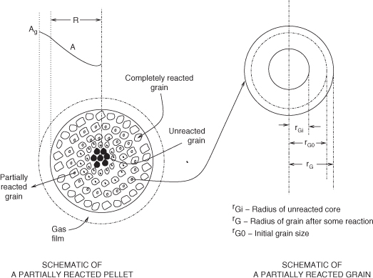
Figure 19.8 Schematic of the concepts used in the particle-pellet model, also known as the grain model. Based on Ramachandran and Doraiswamy, 1977.
Distributed Pore Models
These models are similar in concept to the single pore model but take into account the effect of pore size distribution. Bhatia and Perlmutter (1981), Reyes and Jensen (1987), and Christman and Edgar (1983) provide illustrative examples and are useful sources for further study of this topic. The additional feature of these models is the simultaneous solution of the population balance equation for the pore size distribution. For a detailed review of various models, Ramachandran and Doraiswamy (1982) is a useful reference. An earlier work by Szekely, Evans, and Sohn (1976) is also another useful source.
19.4 Solid–Solid Reactions
Solid–solid reactions are of importance in a number of industrially important processes. A few examples are given below followed by a very brief discussion on modeling of such reactions.
Carbothermic reduction of ores (e.g., NiO + C) is one of the important examples in metallurgical industry. Cement production (tricalcium aluminate formation) is another large-scale application.
19.4.1 Classical Models
Avrami (1939, 1940, 1941) was one of the earliest investigators to study this and proposed a simple model based on nucleation theory. Transformations are often seen to follow a characteristic s-shaped, or sigmoidal, profile where the transformation rates are low at the beginning and the end of the transformation but rapid in between. The initial slow rate can be attributed to the time required for a significant number of nuclei of the new phase to form and begin growing. During the intermediate period the transformation is rapid as the nuclei grow into particles and consume the old phase while nuclei continue to form in the remaining parent phase. Once the transformation begins to near completion there is little untransformed material for nuclei to form in and the production of new particles begins to slow. Further, the particles already existing begin to touch one another, forming a boundary where growth stops.
Model development leads to the following equation for the conversion as a function of time:
X = 1 – exp(–ktn)
The value of n = 4 was assigned in the original Avrami model. The rate constant k was interpreted as
where is the nucleation rate and is the growth rate of the nuclei.
The equation is also known as the Johnson-Mehl-Avrami-Kolmogorov, or JMAK, equation since it appears to have been first derived by Kolmogorov in 1937 but was popularized by Avrami in a series of articles in the Journal of Chemical Physics.
19.4.2 Dalvi-Suresh Contact Point Model
Dalvi and Suresh (2011) proposed a contact point model, the schematic of which is shown in Figure 19.9.
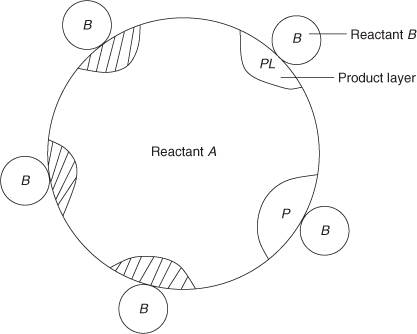
Figure 19.9 Contact points–based model for solid–solid reactions. Based on Suresh and Ghoroi, 2009.
In this model the reaction initiates at points where the reactant B is in contact with A. An ash layer develops in the interior of A near the surface. Further reaction proceeds through the diffusion in the ash layer. If there are a large number of contact points the ash layer overlaps and grows over a region near the surface rather than as discrete islands. In such case the behavior of the system is close to the shrinking core model. On the other hand for a low number of contact points the reaction front consists of several moving fronts within the solid A. Thus the contact point model is able to cover the two limiting cases of reaction control and ash diffusion control depending on the value of the parameters such as the number of contact points and the rate of growth at these contact points.
Summary
Reaction of a gas with a solid is important in several industrial situations. Similar to the gas–catalytic reaction, the rate is affected by mass transfer parameters such as film diffusion and internal diffusion; the modeling approach follows a similar pattern to gas–solid catalytic reactions.
The important difference between catalytic and non-catalytic reactions is that the solid reactant concentration variation needs to be added in the model and the concentration profiles of the gas and solid are changing with time, unlike the case of a catalytic solid.
If the solid is non-porous the reaction is assumed to take place at a sharp interface between the gas (A) and the solid reactant (B) because the gas A does not penetrate into the interior of the non-porous B. Depending on whether a gaseous product or a porous solid product is formed two variations of this model are generally used.
If the product is gaseous, then the shrinking solid model is used where the external film mass transfer and reaction at the solid surface are the two steps that need to be considered. A pseudo-steady state profile for the diffusing gas is usually assumed.
A shrinking core model is also applied when the product of the reaction is a porous solid. A product layer called the ash layer forms on the original solid reactant and adds an extra resistance to mass transfer. Hence three mass transfer steps, film mass transfer, diffusion through the ash layer and reaction at the solid surface, need to be considered in the calculation of the rate.
The change in B concentration is then calculated using a transient mass balance for B. The time versus conversion of the solid can be calculated on the basis of this model. The time for complete conversion for a given particle radius depends on the controlling regime. Time is proportional to particle radius if the reaction kinetics is controlled and it is proportional to radius squared if the ash diffusion is controlling.
A solid can react non-uniformly under certain conditions due to surface irregularity and orientation of the crystal planes in the surface. This can lead to anisotropic growth or etching or wormhole formation. The shrinking core model is not applied for such cases and some alternative models proposed in the literature can be used. An example is etching of semi-conductor wafers with potassium hydroxide solutions.
For porous solids the reaction takes place in the interior surface of the solid. The gas species profile in the solid due to intraparticle diffusion needs to be included in the model. These models are generally called volume reaction models to contrast with the sharp interface models for non-porous solids.
In volume reaction models the reaction does not take place at a sharp interface but is confined to a finite volume. The extent of this volume depends on parameters similar to the Thiele modulus for gas–solid catalytic reactions. If the Thiele modulus is small the gas concentration is nearly uniform in the pellet and reaction takes place all over the solid. Reactant B is consumed uniformly in the pellet. The model based on this is also referred to as a “homogeneous” reaction model.
In volume reaction models, if the Thiele parameter is large, the reaction is initially confined to a zone near the surface of the solid. Reactant B is consumed only here and not near the center. Over time as the B near the surface is consumed, the zone moves inward and finally shifts to a region near the center.
Reactions that are zero order with respect to B exhibit features similar to the catalytic zero-order reaction. If the Thiele parameter is large, reaction takes place in a reaction zone near the surface of the solid. This reaction zone does not move with time until the surface concentration of B drops to zero. Then a B-depleted zone develops near the surface similar to an ash layer and the reaction zone moves inward. Analytic solutions can be developed for the initial time and the later time where the movement of the ash layer has to be tracked as well.
The molar volume ratio parameter is an important parameter in the context of the volume reaction model. If the parameter is large, the pores get smaller with the extent of reaction of the solid. The pore size reduction has to be accounted for by a corresponding change in the effective diffusion coefficient. A number of models have been proposed for this and all these models differ only in the way the pore structure and the variation in diffusion coefficient are handled.
For a certain range of the molar ratio parameter, pore plugging can result and incomplete conversion of the solid is observed. An example is the reaction of SO2 with CaO where pore plugging leads to incomplete utilization of the solid reactant.
Solid–solid reactions have certain additional complications, but concepts from solid–gas reactions are often applied. The classical model of Avrami (1940) discussed in the text is often used in practice. Many of these are reaction networks, and not single-step reactions as normally assumed. There is no complete theoretical framework available for the analysis of such systems. The importance of contact points between the two solids is studied in a number of newer models. For the case where there is a large set of contact points, the solid can react according to the shrinking core model, which provides some justification to the use of solid–gas models even for solid–solid systems.
Review Questions
19.1 When would you use the shrinking solid model?
19.2 When would you use the volume reaction model?
19.3 How does the time for complete conversion depend on the particle radius for the shrinking core model if the reaction is controlling?
19.4 How does the time for complete conversion depend on the particle radius for the shrinking core model if ash layer diffusion is controlling?
19.5 What is meant by the law of addition of time?
19.6 When can you expect wormhole formation or anisotropic etching?
19.7 If the starting solid is relatively porous what type of model would you use?
19.8 Why is the ratio of the molar volume of the product and the reactant important in modeling gas–solid reactions?
19.9 What are the main differences between a gas–solid reaction and a solid–solid reaction?
19.10 What are the common models useful for solid–solid reactions?
Problems
19.1 Cynamide formation from carbide. Calcium carbide reacts with nitrogen to give calcium cynamide by the following reaction:
N2(g) + CaC2(s) → CaCN2(s) + C(s)
Particles of 2 mm reacted in 3 hours while those of 4 mm reacted in 6 hours. Suggest a controlling regime and develop a rate equation.
19.2 Time scales in the shrinking core model. Spherical particles of a reacting solid of 4.8 mm are completely converted to products in 100 min. If the ash layer diffusion coefficient is 1 × 10⁻⁶ m2/s and the surface reaction constant is 0.01 m/s, find the contribution of the ash later and reaction to the time needed for the conversion. Estimate the time for the reaction of a particle of 9.6 mm.
19.3 Reduction of magnetite with hydrogen. Consider reduction of magnetite ore with hydrogen, which is important in direct routes for iron production. The kinetic data is given as
ks = 1930 exp(–E/RgT)
with E = 100, 000 J/mol and ks in m/s. The effective diffusion coefficient is 3 × 10⁻⁶ m2/s in the ash layer. The reaction is carried out in pure hydrogen at 1 atm pressure and 600 K. The initial particle radius is 5 mm and the density of magnetite is 4600 kg/m3. Plot the conversion versus time data and indicate the operating controlling regime.
19.4 Langmuir kinetics. Topochemical reactions with Langmuir kinetics are often encountered when gas A is strongly adsorbed. Assume that the reaction takes place at a sharp interface and the rate of the surface reaction is then represented as kCA(1 + KACA). Develop a shrinking core model for this case.
19.5 Temperature effects on conversion. What is the effect of temperature on conversion? How does the controlling resistance change? The effect of temperature on MgO conversion with carbon was reported by Sohn and Han (2011). The rate increases first with temperature and then decreases with temperature above 975 K. Provide a suitable explanation to this anomalous effect.
19.6 Parameter estimation for the shrinking core model. Find the controlling mechanism for the following time verus conversion data:
Time, Hour |
0.18 |
0.347 |
0.453 |
0.567 |
0.733 |
Conversion |
0.45 |
0.68 |
0.80 |
0.95 |
0.98 |
19.7 Cumulative concentration method for conversion. The model equations for a (1,1) order reaction can be solved in an approximate analytical manner using the concept of cumulative concentration. This exercise walks you through the steps of this method. The analysis borrows the generalized Thiele modulus concept used on gas–solid catalytic reactions. The equations to be solved are repeated here for convenience. Using the pseudo-steady state is represented in slab geometry as
The solid phase balance is
Define a cumulative concentration variable, ψ, as
Show that the concentration of B can now be represented as cB = exp(–ψ). Show that the diffusion-reaction model for the gas, Equation 19.31, can now be written as
and state the boundary conditions to be used. This has a resemblance to a diffusion-reaction problem; hence, show that the following expression for the generalized Thiele modulus can be derived:
Correspondingly a “conversion” effectiveness factor can be defined:
Show that the conversion of the solid at any time is given as the conversion in the absence of diffusion times the above effectiveness factor.
19.8 Effect of solid residence time in a fluid bed roaster. Fluid bed reactors are commonly used in metallurgy. The large-scale units are operated continuously. Since there is spread in residence time, the conversion of the solid depends on the E-curve. Show that the following expression can be derived for the conversion:
Here tf is the time needed for complete conversion for a single particle. If one assumes that the solids are well mixed but segregated, what is the expression for the E-curve? Use this in the previous equation and show that the following equation holds:
Use the model to predict the exit conversion for roasting of pyrrhoites if the mean residence time is 60 min and the time for complete conversion for a single particle is 20 min. Assume that the time for complete conversion is proportional to R1.5.