Chapter 6. Diffusion-Dominated Processes and the Film Model

Search in book...
Toggle Font Controls
Create new playlist

Name your new playlist

Playlist description (optional)
Sign In

Email address

Password

Forgot Password?

or

Continue with Facebook

Continue with Google
Sign Up

Full Name

Email address

Confirm Email Address

Password

or

Continue with Facebook

Continue with Google

Chapter 6. Diffusion-Dominated Processes and the Film Model

Learning Objectives

After completing this chapter, you will be able to:

Solve prototype problems involving steady state diffusion.
Describe how diffusion can cause an associated flow (diffusion-induced convection).
Account for the effect of convection in diffusion-dominated systems (i.e., stagnant systems).
Describe the film theory concept of mass transfer and its usefulness in many applications.
Evaluate how the rate of chemical reaction at a surface is affected by the rate of mass transfer.
Explain the two-film theory for gas–liquid (or liquid–liquid) mass transfer and calculate the rate of interfacial mass transfer given the bulk composition of the two phases.

This chapter examines problems where the diffusion is the main mode of mass transport. Such systems are often referred to as diffusion in stagnant media for analogy with problems of purely heat conduction. However, this does not mean that the convection effects can be totally ignored. The term “stagnant” can therefore be misleading in some cases. Thus, the effect of convection-induced by diffusion is also addressed in this chapter.

A model widely used in mass transport analysis is the film model, which is based on the assumption of a “stagnant” film near a fluid–solid interface. Transport effects are analyzed using either diffusion or diffusion plus diffusion-induced convection as the mode of transport in this film. Detailed effects of the fluid motion near the fluid–solid interface are not considered in this model, but rather are assumed to be buried in the hypothetical parameter called the film thickness. Useful information can be gained from such a model, as illustrated in this chapter.

Film theory can be used to explore a variety of complex situations. An example is the transport of a reactant to a catalyst surface, followed by a heterogeneous reaction. (Another example is simultaneous heat and mass transport which is discussed in Chapter 25). This chapter shows how the heterogeneous reactions can be analyzed using the film model.

The film theory needs a modification for fluid–fluid systems since mass transfer is a sequence of two steps: fluid 1 to interface, and interface to fluid 2. Hence a two-film model (one film on each fluid side of the interface) is used. This model is discussed next and the concept of an overall mass transfer coefficient is introduced. This concept is widely used in modeling and design of separation processes.

Systems in which a chemical reaction takes place at a surface are referred to as heterogeneous reactions; they stand in contrast to systems in which the chemical reaction takes place in the bulk phase of a fluid. The latter are called homogeneous reactions. For heterogeneous reactions, the diffusion applies to the gas phase and the reaction appears only as a boundary condition; that is, the reaction occurs at the surface only and not in the bulk of the gas phase. Hence some aspects of heterogeneous reactions are also studied here, since they are amenable to analysis using film theory. In addition, the role of mass transfer in changing the overall rate is illustrated.

The problems analyzed in this chapter are quite important in practical applications and provide a framework for designing a wide variety of mass transfer and reactor equipment. After a detailed study of this chapter, you will be able to calculate the local rate of mass transport at any given point in mass transfer equipment. In later chapters we will combine this local rate with a macroscopic or mesoscopic model for a system such as a reactor or separator, and we will demonstrate such coupled models for design/simulation of such equipment.

6.1 Steady State Diffusion: No Reaction

This section summarizes the equations for steady state diffusion and discusses the role of diffusion-induced convection. If this convection effect is neglected and a constant diffusion coefficient is assumed, the concentration profile can be determined by the solution of the Laplace equation with appropriate boundary conditions.

6.1.1 Combined Flux Equation

The starting point is the equation of mass transfer. For the present case of steady state and no reaction, the equation simplifies to

\begin{matrix} \nabla \cdot N_{A} = 0 & (6.1) \end{matrix}

$\begin{matrix} \nabla \cdot N_{A} = 0 & (6.1) \end{matrix}$

The flux term N A is the combined flux, which can be expressed as a sum of the diffusion flux and a convection flux:

\begin{matrix} N_{A} = J_{A} + y_{A} N_{t} & (6.2) \end{matrix}

$\begin{matrix} N_{A} = J_{A} + y_{A} N_{t} & (6.2) \end{matrix}$

In this chapter we use Fick’s law for diffusion flux J_A, which is (strictly speaking) valid for ideal binary systems:

J_A = –CD_AΔy_A

Here D_A is the binary pair diffusivity, which is equal to D_AB for a truly binary mixture. For multicomponent mixtures, D_A is interpreted as a pseudo-binary diffusivity D_A–m, which is defined in Equation 5.24.

Hence the equation for N_A can be written as follows:

\begin{matrix} \begin{matrix} N_{A} = - C D_{A} ▽ y A + y A N_{t} \end{matrix} & (6.3) \end{matrix}

$\begin{matrix} \begin{matrix} N_{A} = - C D_{A} ▽ y A + y A N_{t} \end{matrix} & (6.3) \end{matrix}$

The first term is the diffusion flux, and the second term is the convection flux. This, together with the conservation requirement that the divergence of the flux vector should be zero, forms the basis for the solution of the problems examined in this chapter. We consider diffusion as the dominant mode of transport in this chapter. We assume that there is no superimposed flow caused by external means such as a pump or fan. The question then arises as to why the convection is included in this chapter, which specifically deals with diffusion-dominated processes. This question is answered in the following section.

6.1.2 Diffusion-Induced Convection

Consider a liquid evaporating from a container, as shown in Figure 6.1. There is no superimposed flow and the evaporation is mainly due to diffusion caused by the concentration difference in the vapor phase. The evaporation implies some movement of A and, therefore, there is a convective flow due to evaporation. In this case, the term y_AN_t in Equation 6.3 is retained in the model to account for the contribution due to convection. We examined this case in Example 5.1 in Chapter 5, where we found a small but nonzero value for both the velocities v and v*. The contribution due to this flow was not accounted for there, however, and will be considered later in this chapter.

Diagrammatic representation of Diffusion-Induced Convection.

Figure 6.1 Liquid evaporating in a glass. Transport takes place both by diffusion and by convection, although the convective flow is not evident.

6.1.3 Determinacy Condition

The term N_t is equal to sum of the combined flux of all the species. For example, in a binary system, it is equal to N_A + N_B. To close the problem, some additional relation for N_t or N_B has to be independently specified. This is known as the determinacy condition. The specification is situation dependent, and various cases are discussed in more detail in Section 6.3.3. Two common cases are indicated here for a binary mixture.

Unimolecular diffusion (UMD): Second component has no transport. N_B = 0. An example would be a species (A) evaporating into an inert gas (B). Hence N_t is non-zero and diffusion-induced convection needs to be included to create a more exact model. The determinacy condition is therefore N_t = N_A.
Equimolar counter-diffusion (EMD): Second component counter-diffusing with same magnitude of flux N_B = –N_A. An example would be the situation in which species A diffuses to a catalytic surface, reacts to produce an equal mole of B, and then B counter-diffuses to the bulk gas phase. Hence N_t is zero and diffusion-induced convection is not present (using a mole-centric frame of reference).

N_t versus n_t

An alternative way of writing the flux expression is in mass units:

\begin{matrix} n_{A} = - ρ D_{A} \nabla ω A + ω_{A} n_{t} & (6.4) \end{matrix}

$\begin{matrix} n_{A} = - ρ D_{A} \nabla ω A + ω_{A} n_{t} & (6.4) \end{matrix}$

This is a useful representation if ρ is constant across the system. Otherwise, the local variation of ρ has to be included in the calculations. Likewise, the mole unit version given by Equation 6.3 is suitable if the total concentration is a constant in the system.

A useful but sometimes confusing point to note is that if N_t is zero, it does not imply that n_t is also zero. This difference, which was also discussed in Chapter 5, is due to the difference in total mole balance versus total mass balance. It is also a consequence of the different ways of averaging the system velocity. A few examples are given here to illustrate this point.

An example where N_t is zero but n_t is non-zero is equimolar counter-diffusion. Consider a tube that has hydrogen at one end and nitrogen at the other end. The system is maintained at a constant temperature and pressure, so the total molar concentration in the tube is constant. The moles of hydrogen diffusing in one direction is equal to the moles of nitrogen diffusing in the opposite direction, leading to N_t equal to zero. However, there is a net mass flow rate from the nitrogen side to the hydrogen side since nitrogen has a higher molecular weight than hydrogen. Hence n_t is not zero.

Now consider a case where 1 mole of a species A diffuses to a catalytic surface and 2 moles is produced from diffusion in the opposite direction. Here N_t is not zero and n_t is zero, since on a mass basis the chemical reaction creates no change in mass. It is useful to reflect on and appreciate these subtle points. Examples 5.1 to 5.3 in Chapter 5 highlighted these points as well. Ultimately the choice of N_t versus n_t is dependent on which of these will lead to a simpler model.

6.1.4 Low Flux Model: The Laplace Equation

A commonly used model for diffusion-dominated systems is the low flux model, which is defined for our purposes as a model in which the effect of diffusion-induced convection is neglected. In this case, only diffusion flux is included. Thus

\begin{matrix} N_{A} \approx J_{A} = - C D_{A B} \nabla y_{A} & (6.5) \end{matrix}

$\begin{matrix} N_{A} \approx J_{A} = - C D_{A B} \nabla y_{A} & (6.5) \end{matrix}$

Combining Equation 6.5 and Equation 6.1, we have

∇ ⋅ (CD_ABΔy_A) = 0

This is the starting point for steady diffusion problems.

Consider a system at constant concentration—a condition that applies to isobaric and isothermal systems. Also assume that the diffusion coefficient does not vary much across the system, such that a constant value can be assigned to it. Then the equation simplifies to

\begin{matrix} \nabla^{2} y_{A} = 0 & (6.6) \end{matrix}

$\begin{matrix} \nabla^{2} y_{A} = 0 & (6.6) \end{matrix}$

Since the system is at constant concentration, we can also write this equation as

\begin{matrix} \begin{matrix} \nabla^{2} C_{A} = 0 \end{matrix} & (6.7) \end{matrix}

$\begin{matrix} \begin{matrix} \nabla^{2} C_{A} = 0 \end{matrix} & (6.7) \end{matrix}$

Thus the concentration field satisfies the Laplace equation with the assumptions stated earlier. Solution of the Laplace equation is a well-studied problem in engineering mathematics. The form of the Laplacian in three common coordinate systems is shown next.

Expression for the Laplacian of Concentration in Common Coordinate Systems

1. Cartesian coordinates:

\begin{matrix} \nabla \cdot \nabla C_{A} = \nabla^{2} C_{A} = \frac{\partial^{2} C_{A}}{\partial x^{2}} + \frac{\partial^{2} C_{A}}{\partial y^{2}} + \frac{\partial^{2} C_{A}}{\partial z^{2}} & (6.8) \end{matrix}

$\begin{matrix} \nabla \cdot \nabla C_{A} = \nabla^{2} C_{A} = \frac{\partial^{2} C_{A}}{\partial x^{2}} + \frac{\partial^{2} C_{A}}{\partial y^{2}} + \frac{\partial^{2} C_{A}}{\partial z^{2}} & (6.8) \end{matrix}$

2. Cylindrical coordinates:

\begin{matrix} \nabla^{2} C_{A} = \frac{1}{r} \frac{\partial}{\partial r} (r \frac{\partial C_{A}}{\partial r}) + \frac{1}{r^{2}} \frac{\partial^{2} C_{A}}{\partial θ^{2}} + \frac{\partial^{2} C_{A}}{\partial z^{2}} & (6.9) \end{matrix}

$\begin{matrix} \nabla^{2} C_{A} = \frac{1}{r} \frac{\partial}{\partial r} (r \frac{\partial C_{A}}{\partial r}) + \frac{1}{r^{2}} \frac{\partial^{2} C_{A}}{\partial θ^{2}} + \frac{\partial^{2} C_{A}}{\partial z^{2}} & (6.9) \end{matrix}$

3. Spherical coordinates:

\begin{matrix} \begin{matrix} \nabla^{2} C_{A} = \frac{1}{r^{2}} \frac{\partial}{\partial r} (r^{2} \frac{\partial C_{A}}{\partial r}) + \frac{1}{r^{2} \sin θ} \frac{\partial}{\partial θ} (\sin θ \frac{\partial C_{A}}{\partial θ}) \\ + \frac{1}{r^{2} {sin}^{2} θ} \frac{\partial^{2} C_{A}}{\partial ϕ^{2}} \end{matrix} & (6.10) \end{matrix}

$\begin{matrix} \begin{matrix} \nabla^{2} C_{A} = \frac{1}{r^{2}} \frac{\partial}{\partial r} (r^{2} \frac{\partial C_{A}}{\partial r}) + \frac{1}{r^{2} \sin θ} \frac{\partial}{\partial θ} (\sin θ \frac{\partial C_{A}}{\partial θ}) \\ + \frac{1}{r^{2} {sin}^{2} θ} \frac{\partial^{2} C_{A}}{\partial ϕ^{2}} \end{matrix} & (6.10) \end{matrix}$

Solutions to the Laplace equation for some simple situations are presented here to demonstrate the use of this model. Example 6.1 is applicable to a cylindrical geometry.

Example 6.1 Radial Diffusion in a Cylindrical Geometry

Consider the diffusion in cylindrical coordinates with the concentration varying only in the radial direction. Show that the concentration profile is a logarithmic function of the radial coordinate.

Solution

The Laplace equation in cylindrical coordinates is applicable here. Keeping only the variation in r, we get

\begin{matrix} \frac{1}{r} \frac{d}{d} (r \frac{d C_{A}}{d r}) = 0 & (6.11) \end{matrix}

$\begin{matrix} \frac{1}{r} \frac{d}{d} (r \frac{d C_{A}}{d r}) = 0 & (6.11) \end{matrix}$

The first integration gives

(r \frac{d C_{A}}{d r}) = constant = A_{1}

$(r \frac{d C_{A}}{d r}) = constant = A_{1}$

Dividing both sides by r and integrating again, we get

C_A = A₁ ln r + A₂

Hence the profile is a logarithmic function of r. This was also shown in Chapter 2 starting from detailed balances. Here we show the same result starting directly from the general equation for steady state diffusion.

We now study another simple application to a spherical geometry and derive an expression for the transfer coefficient for mass transfer from a sphere to a stagnant gas in Example 6.2.

Example 6.2 Mass Transfer from a Sphere to a Stagnant Gas

A spherical solid (e.g., naphthalene) is subliming into a gas phase (e.g., air) that is stagnant. Derive an expression for the concentration profile in the gas phase and an equation for the rate of evaporation. Use them to obtain an expression for the mass transfer coefficient in the absence of any gas flow.

Solution

Here N_A, the flux of the sublimining solid, is non-zero and the flux of the gas phase (air) is zero. Hence the total flux N_t is non-zero here, as this is the UMD situation. Although diffusion-induced convection will have some effect in this system, if the vapor pressure of the subliming solid is small its contribution to the flux can be neglected and a low flux model used. Hence the Laplace equation in spherical coordinates applies for the gas-phase concentration of A. Keeping only the r-dependent term, we have

\begin{matrix} \frac{1}{r^{2}} \frac{d}{d r} (r^{2} \frac{d C_{A}}{d r}) = 0 & (6.12) \end{matrix}

$\begin{matrix} \frac{1}{r^{2}} \frac{d}{d r} (r^{2} \frac{d C_{A}}{d r}) = 0 & (6.12) \end{matrix}$

This equation can be integrated twice to get a general expression for the concentration profile:

C_{A} = \frac{A_{1}}{r} + A_{2}

$C_{A} = \frac{A_{1}}{r} + A_{2}$

Now we impose two boundary conditions to get A₁ and A₂. We assume that far away from the subliming sphere, the concentration is zero. Hence as r → ∞, we should have C_A = 0. Hence A₂ = 0.

At the sphere surface r = R, the concentration in the gas phase is equal to C_As such that the thermodynamic equlibirum applies at this point:

C_{A s} = \frac{ρ A, υ a p}{R_{g} T}

$C_{A s} = \frac{ρ A, υ a p}{R_{g} T}$

where pA,_vap is the vapor pressure of the subliming solid at the given temperature.

Using this condition the concentration profile in the gas phase is

C_{A} = C_{A s} \frac{R}{r}

$C_{A} = C_{A s} \frac{R}{r}$

The flux at the solid surface is the rate of evaporation per unit area of the solid. It is calculated by applying Fick’s law at the surface:

N_{A s} = - D_{A} {(\frac{d C_{A}}{d r})}_{r = R}

$N_{A s} = - D_{A} {(\frac{d C_{A}}{d r})}_{r = R}$

Using the concentration profile and its derivative at r = R, the following expression for the flux is obtained:

N_{A s} = \frac{D_{A}}{R} \cdot C_{A s}

$N_{A s} = \frac{D_{A}}{R} \cdot C_{A s}$

If one writes the flux as a product of the mass transfer coefficient times the driving force, the following result is obtained for the mass transfer coefficient:

\begin{matrix} \begin{matrix} k_{m} = \frac{N_{A s}}{C_{A s}} = \frac{D_{A}}{R} \end{matrix} & (6.13) \end{matrix}

$\begin{matrix} \begin{matrix} k_{m} = \frac{N_{A s}}{C_{A s}} = \frac{D_{A}}{R} \end{matrix} & (6.13) \end{matrix}$

This equation sets a base value for the mass transfer coefficient for mass transfer from solid to gas in the absence of any superimposed external flow in the gas phase. The effect of the superimposed external flow is then fitted by adding an extra term, which depends on the Reynolds number. (See the discussion of the Ranz-Marshall correlation in Section 3.4.)

6.2 Diffusion-Induced Convection

In this section, we study the correction needed to account for diffusion-induced convection. First we discuss conditions in which the diffusion-induced convection can be neglected and the low flux model can be applied. This is followed by an analysis of diffusion-induced convection for the UMD case.

6.2.1 Conditions for the Validity of the Low Flux Model

The low flux model holds when the diffusive component of the combined flux is much larger than the convection flux—that is, when

J_A >> y_AN_t

This can happen, for example, when N_t is small (i.e., low mass transfer flux) or when y_A is small (dilute systems). In these cases it is fine to consider diffusion only.

Note: The diffusion component is the only term to be considered when N_t is zero due to the nature of the problem. In this case, which is known as EMD, two species diffuse at the same rate but in opposite directions. The net flux is then automatically zero even if y_A is large. The low flux model applies then, although the magnitude of the flux need not be low.

In general, it is necessary to define the total flux N_t independently, by specifying the determinacy condition. We now show this case for UMD. More examples of determinacy conditions for other cases are provided in Section 6.3.3.

6.2.2 Analysis for UMD

UMD (unimolecular diffusion) refers to the case in which only one species (say, A) has a non-zero flux; that is, the component B has no flux in a stationary frame of reference. Hence N_B = 0 and N_A + N_B = N_t = N_A, which is the determinacy condition for the UMD situation.

The expression for the combined flux can now be written as

\begin{matrix} N_{A} = - C D_{A B} \nabla y_{A} + N_{A} y_{A} & (6.14) \end{matrix}

$\begin{matrix} N_{A} = - C D_{A B} \nabla y_{A} + N_{A} y_{A} & (6.14) \end{matrix}$

Rearranging, we have the flux expression for UMD:

\begin{matrix} N_{A} = - \frac{C D_{A B}}{(1 - y_{A})} \nabla y_{A} & (6.15) \end{matrix}

$\begin{matrix} N_{A} = - \frac{C D_{A B}}{(1 - y_{A})} \nabla y_{A} & (6.15) \end{matrix}$

Note the presence of the 1 – y_A term in the denominator. This term is equal to 1 in the low flux model, if the diffusion-induced convection is neglected.

For the one-dimensional case, ∇y_A = dy_A/dz, where z is the direction of diffusion. Hence the flux expression can be written after separating the variables as

\begin{matrix} N_{A} d z = - C D_{A B} \frac{d y_{A}}{1 - y_{A}} & (6.16) \end{matrix}

$\begin{matrix} N_{A} d z = - C D_{A B} \frac{d y_{A}}{1 - y_{A}} & (6.16) \end{matrix}$

N_A (no boldface) is used as an abbreviation for the z-component of the flux vector, N_Az.

The expression for the evaporation rate for the system shown in Figure 6.1 will now be derived including the diffusion induced correction, Integrating Equation 6.16 across the vapor space and keeping N_A constant (as required to satisfy Equation 6.1), we get the rate of evaporation:

\begin{matrix} \begin{matrix} N_{A} = - \frac{C D_{A B}}{H} \ln (\frac{1 - y_{A s}}{1 - y_{A b}}) \end{matrix} & (6.17) \end{matrix}

$\begin{matrix} \begin{matrix} N_{A} = - \frac{C D_{A B}}{H} \ln (\frac{1 - y_{A s}}{1 - y_{A b}}) \end{matrix} & (6.17) \end{matrix}$

where y_As is the mole fraction at the evaporating surface z = 0 and y_Ab is the mole fraction in the bulk gas—that is, at z = H and beyond. (H is the height of the vapor space in the evaporating tube.)

For the commonly used case of y_Ab equal to zero, Equation 6.17 reduces to

\begin{matrix} N_{A} = - \frac{C D_{A B}}{H} \ln (1 - y_{A s}) & (6.18) \end{matrix}

$\begin{matrix} N_{A} = - \frac{C D_{A B}}{H} \ln (1 - y_{A s}) & (6.18) \end{matrix}$

Note that the flux is not linear to the driving force.

Now if y_As is small we can make the following approximation for the log term:

ln(1 – x) ≈ –x as x → 0

The model then reduces to the low flux case:

\begin{matrix} N_{A} = \frac{C D_{A B} y_{A s}}{H} & (6.19) \end{matrix}

$\begin{matrix} N_{A} = \frac{C D_{A B} y_{A s}}{H} & (6.19) \end{matrix}$

The flux is now linearly proportional to the mole fraction gradient.

The comparison of Equations 6.18 and 6.19 also helps us to ascertain the validity of the diffusion-only model. For example, if y_As = 0.1, then the convection model would give a driving force of ln(1 – y_As) = 0.1054. Thus the convection effect can be neglected for dilute systems. If the value of y_As is 0.2, then the factors are 0.2231 (convection included) versus 0.2 (convection neglected) and the error is in the range of less than 10%.

Another way to compare the two approaches is by using the drift flux correction factor, as explained in the following subsection.

6.2.3 Drift Flux Correction Factor

The expression given by Equation 6.17 for a high flux model can be compared with the low mass flux model directly to ascertain the effect of “flow” in the system. The correction factor due to flow (this is ratio of the actual flux to the flux calculated neglecting the diffusion induced convection) can be expressed as a drift flux factor and the following expression can be derived:

\begin{matrix} Correction factor F = \frac{N_{A}}{N_{A}^{\circ}} = \frac{\ln [(1 - y_{A s}) / (1 - y_{A b}]}{y_{A b} - y_{A s}} & (6.20) \end{matrix}

$\begin{matrix} Correction factor F = \frac{N_{A}}{N_{A}^{\circ}} = \frac{\ln [(1 - y_{A s}) / (1 - y_{A b}]}{y_{A b} - y_{A s}} & (6.20) \end{matrix}$

The correction factor can also be written in terms of the mole fraction of B using the relation y_B = 1 – y_A:

F = \frac{\ln (y_{B s} - y_{B b})}{y_{B s} - y_{B b}} = \frac{1}{log mean value of mole fraction of B .}

$F = \frac{\ln (y_{B s} - y_{B b})}{y_{B s} - y_{B b}} = \frac{1}{log mean value of mole fraction of B .}$

where the log mean is defined as

log mean y B = \frac{y B b - y B s}{In (y B b / y B s)}

$log mean y B = \frac{y B b - y B s}{In (y B b / y B s)}$

We can compare the effects of drift by examining a simple example, as shown in Example 6.3.

Example 6.3 Drift Correction to Low Flux Model

A volatile liquid is present in a tube with an exposed vapor height of 0.3 m. The vapor pressure is 0.15 atm at the given conditions of 35° C and 1 atm pressure. The diffusion coefficient is estimated as 8.8 × 10^–6 m²/s. Find the rate of evaporation.

Solution

The following quantities can be calculated:

Total concentration, C = P/R_gT : 39.56 mol/m³
Flux from low flux model, given by Equation 6.19: 1.04 × 10^–4 mol/m²s
Flux from high flux model, given by Equation 6.18: 1.1318 × 10^–4 mol/m²s
Correction factor: the ratio of the two and equal to 1.1230; thus convection augments diffusive transport by about 12%.

The correction factor can also be ascertained by calculating the log mean mole fraction of the inert component. We have y_Bs = 1 – 0.15 – 0.85 and y_Bb = 1.0. Hence the log average of these is found as (1 – 0.85) / log (1/0.85) = 0.9230.

The correction factor is then equal to the reciprocal of this log mean: 1/0.9230 = 1.1230. Both procedures give the same answer, as expected.

6.2.4 Mole Fraction Profiles in UMD

The flux expression was derived by integrating across the system—that is, from 0 to H. The mole fraction profile need not be computed in this case to get the flux. The calculation of the mole fraction profile requires a partial integration from 0 to z and is shown in this section.

To find the mole fraction profile, Equation 6.16 is integrated from 0 to any arbitrary position z, rather than across the complete system:

\begin{matrix} N_{A} \int_{0}^{z} d z = - C D_{A B} \int_{y_{A s}}^{y_{A}} \frac{d y_{A}}{1 - y_{A}} & (6.21) \end{matrix}

$\begin{matrix} N_{A} \int_{0}^{z} d z = - C D_{A B} \int_{y_{A s}}^{y_{A}} \frac{d y_{A}}{1 - y_{A}} & (6.21) \end{matrix}$

The integrated version is

zN_A = CD_ABln[(1 – y_A)/(1 – y_As)]

This can be rearranged to the following form for the mole fraction profile:

\begin{matrix} y_{A} = 1 - (1 - y_{A s}) \exp (\frac{z N_{A}}{C D_{A}}) & (6.22) \end{matrix}

$\begin{matrix} y_{A} = 1 - (1 - y_{A s}) \exp (\frac{z N_{A}}{C D_{A}}) & (6.22) \end{matrix}$

Note that the profile is no longer linear, in contrast to the result with the low flux model.

An illustrative comparison is shown in Figure 6.2 in which we use a y_As value of 0.5 (a rather large vapor pressure intended to show the convection effects). Note that the profile is not linear when the convection effect is included.

Graphical representation of data related to comparing concentration profiles with low flux and high flux.

Figure 6.2 Evaporation in a tube: comparison of concentration (mole fraction) profiles with the low flux and high flux models. y_As = 0.5 and y_Ab = 0. Flux is scaled by D_AC/H.

In Example 6.4, the flux model shown earlier is coupled with a macroscopic balance for the second phase (the liquid).

Example 6.4 Liquid Evaporating in an Open Container

A schematic of the problem of evaporation in a tube was shown in Figure 6.1. Determine how the liquid level in the tube changes as a function of time.

Solution

An apparatus of this type is called an Arnold cell (or sometimes a Stefan cell). The level decreases as a function of time in the Arnold cell, and this change in level can be used to determine the diffusivity of the evaporating gas in the carrier gas. This is actually a transient diffusion problem, but for modeling purposes we focus on a particular instant in time when the vapor space has a height H and assume a steady state. This assumption, called the pseudo-steady state hypothesis, holds when the time scale for level changes is much larger than the time scale for diffusion. We will calculate the rate of mass transfer based on this assumption.

A transient mass balance for the liquid phase is now used:

in – out = accumulation

The in term is zero and the out term is the rate of evaporation in mol/s units. This rate is given as AN_A, where A is the cross-sectional area of the container. Accumulation is the time derivative of moles of A in the liquid at any instant of time. (This will be a negative quantity in this example.) The number of moles in the container at any instant of time is ρ_LA(L – H)/M_A, where L is the height of the container.

Putting all this information together, you should show that

\frac{d H}{d t} = \frac{M_{A}}{ρ_{L}} N_{A}

$\frac{d H}{d t} = \frac{M_{A}}{ρ_{L}} N_{A}$

where N_A is the instantaneous rate of evaporation—that is, the rate of evaporation based on the current height of vapor space H:

N_{A} = \frac{D_{A} C y_{A s}}{H} F

$N_{A} = \frac{D_{A} C y_{A s}}{H} F$

where $F$ $F$ is the drift correction factor. In this expression we assume that the bulk mole fraction of A (at the tube edge and outside the tube) is zero.

Substituting and integrating, the height change is given as

H^{2} - H_{0}^{2} = 2 \frac{M_{A}}{ρ_{L}} D_{A} C y_{A s} F t

$H^{2} - H_{0}^{2} = 2 \frac{M_{A}}{ρ_{L}} D_{A} C y_{A s} F t$

6.3 Film Concept in Mass Transfer Analysis

The equation for flux—Equation 6.17 for instance—is derived for the evaporation of a liquid but finds wide application in the field of mass transfer. In this section, we discuss the classical film theory for mass transfer where such equations find use. The film model attempts to provide a simplified representation of mass transfer across a fluid–solid interface. The film model can be viewed as a simplified representation of the mass transport phenomena taking place near a fluid–solid boundary.

More detailed models use the convection–diffusion equation and the concept of a boundary layer near the solid–fluid interface (discussed in Chapter 11). The film model is simpler, however, and is also useful to incorporate the coupling between mass transfer and reaction. We review the boundary layer concepts here briefly to establish the background for understanding the film model.

6.3.1 Boundary Layer Concept for Fluid–Solid Mass Transfer

Near a solid surface there is a boundary layer where the velocity changes from zero to a bulk value over a small distance known as the hydrodynamic boundary layer. Similarly, there is a region where the concentration changes, called the mass transport boundary layer. Typical concentration profiles in the boundary layer are shown in Figure 6.3.

Diagrammatic representation of the concept of hydrodynamic layer.

Figure 6.3 Concentration profile near a solid surface and its approximation by the film model. Solid lines are profiles as envisaged by boundary layer theory; the dashed line is an approximation according to the film model.

Results from Boundary Layer Theory for a Flat Plate

Key results for the mass transfer coefficient needed from the boundary layer theory are summarized here and more details are studied in Chapter 11. The results are useful to understand the film concepts in mass transfer. We will assume that we have a laminar boundary layer—that is, that the flow within the boundary layer is laminar and has no fluctuating velocity components.

The flux at the surface is approximated as a low flux value with Fick’s law:

\begin{matrix} N_{A} = boundary layer model model = - D_{A} {(\frac{d C_{A}}{d y})}_{y = 0} & (6.23) \end{matrix}

$\begin{matrix} N_{A} = boundary layer model model = - D_{A} {(\frac{d C_{A}}{d y})}_{y = 0} & (6.23) \end{matrix}$

The concentration gradient at the surface can be calculated by a detailed model, which is discussed in Chapter 11. This detailed approach is called Blasius analysis.

The concentration profile is often approximated as a cubic polynomial. The following approximation (known as the von Karman approximation and studied in more detail in Chapter 11) is a reasonable representation:

\begin{matrix} c A = \frac{C_{A} - C_{A S}}{C_{A b} - C_{A s}} = \frac{3}{2} \frac{y}{δ_{m}} - \frac{1}{2} (\frac{y}{δ_{m}})^{3} & (6.24) \end{matrix}

$\begin{matrix} c A = \frac{C_{A} - C_{A S}}{C_{A b} - C_{A s}} = \frac{3}{2} \frac{y}{δ_{m}} - \frac{1}{2} (\frac{y}{δ_{m}})^{3} & (6.24) \end{matrix}$

where δ_m is the thickness of the boundary layer for mass transfer. Note that this relation holds only if the flow in the boundary layer is laminar. An expression for the boundary layer thickness δ_m can be derived as shown later.

The flux at y = 0 can be calculated using this cubic profile:

N_{A 0} = \frac{3}{2} \frac{D_{A}}{δ_{m}} (C_{A s} - C_{A b})

$N_{A 0} = \frac{3}{2} \frac{D_{A}}{δ_{m}} (C_{A s} - C_{A b})$

Using the definition of the mass transfer coefficient, we can write this expression as

N_A₀ = k_m(C_As – C_Ab)

Comparing the two expressions, the mass transfer coefficient is predicted from this equation as

\begin{matrix} k_{m} = \frac{3}{2} \frac{D}{δ_{m}} & (6.25) \end{matrix}

$\begin{matrix} k_{m} = \frac{3}{2} \frac{D}{δ_{m}} & (6.25) \end{matrix}$

This is a local mass transfer coefficient at any position x along the flat plate. It varies along the plate since δ, the thickness of the hydrodynamic boundary layer, and δ_m, the mass transfer boundary layer, are both functions of x.

Relation to Momentum Boundary Layer

The mass transfer boundary layer thickness, δ_m, is often correlated as a function of the momentum boundary layer thickness, δ, and the Schimdt number defined as ν/D_A:

δ_{m} = \frac{δ}{S c^{1 / 3}}

$δ_{m} = \frac{δ}{S c^{1 / 3}}$

By using this definition in Equation 6.25, we can relate the mass transfer coefficient to the Schmidt number:

\begin{matrix} k_{m} = \frac{3}{2} \frac{D}{δ} S c^{- 1 / 3} & (6.26) \end{matrix}

$\begin{matrix} k_{m} = \frac{3}{2} \frac{D}{δ} S c^{- 1 / 3} & (6.26) \end{matrix}$

An example of the use of this equation is provided in Example 6.5.

Example 6.5 Mass Transfer Coefficient for a Flat Plate with Laminar Flow

A gas stream is flowing past a plate at a velocity of 0.8 m/s. Estimate the value of the mass transfer coefficient at a distance 0.5 m from the leading edge of the plate. Assume the flow is laminar.

Solution

The physical properties needed are the kinematic viscosity and the diffusion coefficient. We use the following values: D_A = 6 × 10^–6 m²/s; ν = 1.57 × 10^–5 m²/s. Hence the Schmidt number is ν/D_A = 2.6.

Using momentum transfer theory, the boundary layer thickness for the momentum can be approximated as

δ = 4.6 4 \sqrt{\frac{x ν}{v_{\infty}}}

$δ = 4.6 4 \sqrt{\frac{x ν}{v_{\infty}}}$

Substituting the values of the parameters, the hydrodynamic boundary layer thickness, δ, can be calculated as 0.0145 m.

The mass transfer boundary layer thickness is δ/Sc^1/3. In this example, its value is 0.0105 m. The mass transfer coefficient is now calculated using Equation 6.26; its value is 8.52 × 10^–4 m/s. This is the local value at a position 0.5 m from the leading edge of the plate. The average value can be shown as twice this value.

Why Use the Film Model?

The convection model is a useful predictive tool for the mass transfer coefficient for ideal, well-defined hydrodynamic situations. However, this model becomes cumbersome for some complex situations, such as for turbulent flow, complex geometries, and similar situations. In the context of using the same model format for all these cases and to include additional complexities such as the effect of a chemical reaction, high flux correction, and so on, a simpler model for mass transfer is useful, in contrast to the detailed convection–diffusion model based on the boundary layer theory. The film model provides such a platform and is now discussed.

6.3.2 Film Model Approximation

The film model provides a simple description of mass transport from a solid to a fluid, or vice versa. If a straight line is used to represent the concentration profile in Figure 6.3, we can assume that there is a region of thickness δ_f over which the concentration profile changes. Outside this thickness, we assume a constant concentration equal to the bulk fluid concentration.

Using Fick’s law, the flux can be represented as follows:

\begin{matrix} N_{A}^{o} = \frac{D_{A}}{δ_{f}} (C_{A s} - C_{A b}) & (6.27) \end{matrix}

$\begin{matrix} N_{A}^{o} = \frac{D_{A}}{δ_{f}} (C_{A s} - C_{A b}) & (6.27) \end{matrix}$

Representation of the concentration distribution by a linear function and the concept of the film thickness parameter δ_f forms the basis for the film model for mass transfer. This model was first proposed by Nernst (1904). Although the film is a hypothetical concept, it has enjoyed widespread success in modeling mass transport processes, as we will observe during the course of this chapter.

Equivalently, a mass transfer coefficient can be defined to characterize the mass transfer near a solid with a flow past the solid:

\begin{matrix} N_{A}^{o} = k_{m}^{o} (C_{A s} - C_{A b}) & (6.28) \end{matrix}

$\begin{matrix} N_{A}^{o} = k_{m}^{o} (C_{A s} - C_{A b}) & (6.28) \end{matrix}$

The mass transfer coefficient is therefore related to the film thickness by

\begin{matrix} k_{m}^{o} = \frac{D_{A}}{δ_{f}} & (6.29) \end{matrix}

$\begin{matrix} k_{m}^{o} = \frac{D_{A}}{δ_{f}} & (6.29) \end{matrix}$

The superscript ∘ indicates that the coefficient is based on Fick’s law and is therefore applicable to low flux conditions.

In Example 6.5, the average mass transfer coefficient is 1.7 × 10^–3 m/s. We find a film thickness of 3.5 mm (D/k_m).

If the low flux mass transfer model is not applicable, the flux can be defined as the low flux rate times a correction factor:

\begin{matrix} N_{A} = k_{m}^{∘} (C_{A s} - C_{A b}) F_{m} & (6.30) \end{matrix}

$\begin{matrix} N_{A} = k_{m}^{∘} (C_{A s} - C_{A b}) F_{m} & (6.30) \end{matrix}$

The correction factor depends on the prevailing situation—mainly on which other species are being transported. The correction factor is given by Equation 6.20 for UMD as before. It is equal to 1 for EMD since N_t is zero in this case.

An expression for the correction factor can be presented in a rather general way, as explained in the following discussion. Let us first see what the concentration profile looks like in presence of (diffusion-induced) convection, as shown in Example 6.6.

Example 6.6 Concentration Profiles in the Film

Derive an expression for the concentration profile for the film model that includes convection effects. Also relate the flux of A to the total flux in the system.

Solution

The problem and the associated boundary conditions are sketched in Figure 6.4. The mole fraction of A is y_A₀ in the bulk gas and y_Aδ at the surface. The flux of A is to be computed. The expressions for the combined flux is used in presence of convection. Thus we have

\begin{matrix} N_{A} = - C D \frac{d y_{A}}{d z} + y_{A} N_{t} & (6.31) \end{matrix}

$\begin{matrix} N_{A} = - C D \frac{d y_{A}}{d z} + y_{A} N_{t} & (6.31) \end{matrix}$

Diagrammatic representation shows the film model showing a species A diffusing to a solid surface, related to the problem statement.

Figure 6.4 Schematic of the film model to derive a general flux expression. Species A is diffusing to a solid surface. Species B, C, and so on also diffuse or counter-diffuse, which sets up a net total flux N_t, which can be expressed as β times N_A. The dashed line is the profile for β = 0.

Here N_A is the abbreviation for N_Az and not a vector.

Equation 6.31 can be put in a dimensionless form. If we use CD/δ as a scaling parameter for the fluxes, the resulting expression is

\begin{matrix} N_{A}^{*} = - \frac{d y_{A}}{d ζ} + y_{A} N_{t}^{*} & (6.32) \end{matrix}

$\begin{matrix} N_{A}^{*} = - \frac{d y_{A}}{d ζ} + y_{A} N_{t}^{*} & (6.32) \end{matrix}$

Here ζ is the dimensionless distance in the film z/δ and the starred fluxes are dimensionless fluxes.

The component $N_{A}^{*}$ $N_{A}^{*}$ is a constant and not a function of ζ (since we are assuming no reaction taking place simultaneously with diffusion). Hence we can integrate the previous differential equation. Integration and use of the boundary condition y_A₀ at ζ = 0 lead to

\begin{matrix} y_{A} = \frac{N_{A}^{*}}{N_{t}^{*}} + (y_{A 0} - \frac{N_{A}^{*}}{N_{t}^{*}}) \exp (N_{t}^{*} ζ) & (6.33) \end{matrix}

$\begin{matrix} y_{A} = \frac{N_{A}^{*}}{N_{t}^{*}} + (y_{A 0} - \frac{N_{A}^{*}}{N_{t}^{*}}) \exp (N_{t}^{*} ζ) & (6.33) \end{matrix}$

Now we use the boundary condition at ζ = 1, which is y = y_Aζ, and then rearrange to obtain the following equation for N_A:

\begin{matrix} N_{A}^{*} = N_{t}^{*} (\frac{y_{A δ} - y_{A 0} \exp (N_{t}^{*})}{1 - \exp (N_{t}^{*})}) & (6.34) \end{matrix}

$\begin{matrix} N_{A}^{*} = N_{t}^{*} (\frac{y_{A δ} - y_{A 0} \exp (N_{t}^{*})}{1 - \exp (N_{t}^{*})}) & (6.34) \end{matrix}$

This expression can be used for a wide range of problems with a suitable condition specified for N_t as shown below.

Further let

N_{t}^{*} = β N_{A}^{*}

$N_{t}^{*} = β N_{A}^{*}$

Here β is a constant (determinacy correction factor) determined by the total flux condition. For example, β = 1 for UMD and β = 0 for EMD.

Rearranging Equation 6.34, we get a general relation for $N_{A}^{*}$ $N_{A}^{*}$ :

\begin{matrix} \begin{matrix} N_{A}^{*} = \frac{1}{β} \ln (\frac{1 - β y_{A δ}}{1 - β y_{A 0}}) \end{matrix} & (6.35) \end{matrix}

$\begin{matrix} \begin{matrix} N_{A}^{*} = \frac{1}{β} \ln (\frac{1 - β y_{A δ}}{1 - β y_{A 0}}) \end{matrix} & (6.35) \end{matrix}$

This equation is useful for a number of applications, as shown in the following discussion. The actual (dimensional) flux can be calculated by multiplying $N_{A}^{*}$ $N_{A}^{*}$ by (D/δ_f)C or by k_mC.

6.3.3 Film Model: Determinacy Correction Factor

The conditions for N_t and the corresponding value of β to use in Equation 6.35 can be stated on a case-by-case basis. Some common cases and the relations are shown here:

Low flux mass transfer. Taking the limit of Equation 6.35 as β → 0, we have

$\begin{matrix} N_{A}^{*} = (y_{A 0} - y_{A δ}) & (6.36) \end{matrix}$ $\begin{matrix} N_{A}^{*} = (y_{A 0} - y_{A δ}) & (6.36) \end{matrix}$

which can also be obtained by direct application of Fick’s law. The concentration (mole fraction) profile is linear here.
UMD or evaporation of a pure liquid (also called Arnold diffusion). We use $N_{i}^{*} = N_{A}^{*}$ $N_{i}^{*} = N_{A}^{*}$ here, and β = 1 and the following equation hold from Equation 6.35:

$\begin{matrix} N_{A}^{*} = \ln (\frac{1 - y_{A δ}}{1 - y_{A 0}}) & (6.37) \end{matrix}$ $\begin{matrix} N_{A}^{*} = \ln (\frac{1 - y_{A δ}}{1 - y_{A 0}}) & (6.37) \end{matrix}$

You should verify that this is a dimensionless version of Equation 6.17.
EMD or equimolar counter-diffusion. Here N_t = 0 and correspondingly β = 0. The diffusion-induced convective flow is absent. The result for $N_{A}^{*}$ $N_{A}^{*}$ is the same as that for low flux mass transfer.
Distillation of a binary mixture. Here a species A evaporates from a liquid interface to the vapor and a species B condenses from the vapor. No heat is generally added in the distillation column itself. (All heat is added in the reboiler and removed in the condenser.) Hence the heat needed to vaporize A and B must balance, which provides the determinacy condition:

N_A ΔH_vA + N_B ΔH_vB = 0

which relates N_A and N_B. Now N_t can be found and β takes the following value:

$β = 1 - \frac{Δ H_{v A}}{Δ H_{v B}}$ $β = 1 - \frac{Δ H_{v A}}{Δ H_{v B}}$

If the heats of vaporization of A and B are equal, then the equimolar counter-diffusion model holds.
Diffusion with a heterogeneous reaction at a surface. N_A and N_B are determined by the stoichiometry of the reaction. For example, consider a reaction scheme

A → (ν_E + 1)B

where the stoichiometric coefficient for B is written in a funny way for ease of later algebra. The stoichiometry requires

N_B = –(ν_E + 1)N_A

Hence

$\begin{matrix} N_{t} = N_{A} + N_{B} = N_{A} - (ν_{E} + 1) N_{A} = - ν_{E} N_{A} & (6.38) \end{matrix}$ $\begin{matrix} N_{t} = N_{A} + N_{B} = N_{A} - (ν_{E} + 1) N_{A} = - ν_{E} N_{A} & (6.38) \end{matrix}$

Equation 6.35 can now be used with β = –ν_E to find N_A. But we also need a surface reaction boundary condition to calculate the concentration of A at the reacting surface, y_Aδ. See Section 6.4.3 for details.

Thus, the various cases of diffusion-induced convection can be analyzed depending on how N_t and N_A are related. The film model provides a simple but useful platform to perform this analysis.

6.4 Surface Reactions: Role of Mass Transfer

In this section we study diffusion followed by a heterogeneous reaction, and we illustrate how the film model is useful to study the role of mass transfer. A schematic of the problem is shown in Figure 6.5, which illustrates the simple case in which species A diffuses to the surface and forms products that then counter-diffuse back to the bulk gas.

Diagrammatic representation of diffusion followed by heterogeneous reaction, where resultant products diffuse back and the role of mass transfer.

Figure 6.5 Schematic of the steps in mass transfer accompanied by a heterogeneous reaction or chemical vapor deposition on a substrate surface.

6.4.1 Low Flux Model: First-Order Reaction

If diffusion followed by a surface chemical reaction occurs under low flux conditions, then the mass transfer and reaction can be treated as two resistances in series. Let k_s be the rate constant for the reaction. The flux to the surface is equal to the rate of consumption by the reaction. Thus

\begin{matrix} N_{A} = k_{m} (C_{A b} - C_{A s}) = k_{s} C_{A s} & (6.39) \end{matrix}

$\begin{matrix} N_{A} = k_{m} (C_{A b} - C_{A s}) = k_{s} C_{A s} & (6.39) \end{matrix}$

The last two pairs can be used to eliminate C_As:

\frac{C_{A s}}{C_{A b}} = \frac{1}{1 + k_{s} / k_{m}} = \frac{k_{m}}{k_{s} + k_{m}}

$\frac{C_{A s}}{C_{A b}} = \frac{1}{1 + k_{s} / k_{m}} = \frac{k_{m}}{k_{s} + k_{m}}$

The rate can then be expressed in terms of an overall rate constant k_o:

\begin{matrix} N_{A} = k_{o} C_{A b} & (6.40) \end{matrix}

$\begin{matrix} N_{A} = k_{o} C_{A b} & (6.40) \end{matrix}$

where k_o is

\begin{matrix} k_{0} = \frac{k_{m} k_{s}}{k_{s} + k_{m}} & (6.41) \end{matrix}

$\begin{matrix} k_{0} = \frac{k_{m} k_{s}}{k_{s} + k_{m}} & (6.41) \end{matrix}$

This can also be expressed as

\begin{matrix} \frac{1}{k_{o}} = \frac{1}{k_{m}} + \frac{1}{k_{s}} & (6.42) \end{matrix}

$\begin{matrix} \frac{1}{k_{o}} = \frac{1}{k_{m}} + \frac{1}{k_{s}} & (6.42) \end{matrix}$

In this expression, it appears as if two resistances are being added, which is indeed the case. Thus the mass transfer and the reaction resistances operate in series, and the overall resistance is the sum of these two resistances.

The following limiting cases are useful to understand:

Reaction-limiting regime: If k_m >> k_s, then k₀ = k_s; the process is limited by the rate of reaction.
Mass transfer–limiting regime: If k_s >> k_m, then k₀ = k_m; the process is limited by the rate of mass transfer.

The resistance concept does not apply for nonlinear kinetics, as shown in Section 6.4.2.

Measured versus True Kinetics

If the mass transfer resistance is much larger than the reaction resistance, it is not possible to determine k_s accurately from measured experimental data. What you measure is then an indication of the mass transfer coefficient k_m rather than the true rate constant.

In general, the measured rate of reaction can be expressed in terms of an apparent rate constant k_o that is equal N_A/C_Ab (assuming a first-order reaction). This is a combined parameter involving both the true rate constant k_s mass transfer coefficient k_m; it is not a true rate constant of the reaction. To isolate these values and report the true rate constant from the measured reaction rate data, one needs an estimate of the mass transfer coefficient and a correction for the effect of mass transfer. Increasing the gas velocity, and thereby increasing k_m, is one way of reducing the mass transfer resistance. An example of growth of an oxide layer over a silicon surface is shown in Example 6.7.

Example 6.7 Silicon Oxidation: Growth of an Oxide Layer

Growth of an oxide layer over a silicon surface is important in semiconductor processing. Here oxygen diffuses through a product layer of SiO₂ and reaches the SiO₂-Si interface reacts there. Assume a fast reaction. Find how the thickness of the oxide layer changes with time. The problem is shown in Figure 6.6.

Diagrammatic representation of silicon-oxidation process to study the rate of growth of oxide layer.

Figure 6.6 Schematic of the silicon oxidation problem and the study of the rate at which the oxide layer grows.

Solution

The oxygen concentration at the interface is nearly zero for a fast reaction. The process is therefore assumed to be limited by the mass transfer rate. In turn, the rate of oxidation is equal to the rate at which oxygen reaches the surface:

N_{A} = \frac{D}{δ} C_{A s}

$N_{A} = \frac{D}{δ} C_{A s}$

The silicon oxide layer forms with time, and a mass balance for the silicon gives an expression for the thickness of the layer. A balance over the silicon remaining at any time, t, is now done.

in – out + generation = accumulation

No silicon is entering or leaving the control volume. Hence the in and out terms are zero. The balance simplifies to

generation = accumulation

The generation term will be negative here because silicon is actually being consumed by reaction. This, in turn, is equal to the negative of the amount of oxygen arriving at the surface since one mole of oxygen is needed to oxidize one mole of silicon. Hence

Generation = –N_AA

The accumulation is $\frac{d}{d t} [A {(L - δ)}_{ρ B} / M_{B}]$ $\frac{d}{d t} [A {(L - δ)}_{ρ B} / M_{B}]$ , where L is the initial depth of silicon. Equating the two we get

- N_{A} A = - A \frac{d}{d t} [δ_{ρ B} / M_{B}]

$- N_{A} A = - A \frac{d}{d t} [δ_{ρ B} / M_{B}]$

Using the diffusion model for N_A we get

(ρ_{B} / M_{B}) \frac{d δ}{d t} = D_{A} \frac{C_{A s}}{δ}

$(ρ_{B} / M_{B}) \frac{d δ}{d t} = D_{A} \frac{C_{A s}}{δ}$

Integration gives us the relation for the oxide growth layer:

δ = \sqrt{\frac{2 M_{B} D_{A} C_{A s} t}{ρ_{B}}}

$δ = \sqrt{\frac{2 M_{B} D_{A} C_{A s} t}{ρ_{B}}}$

The film thickness increases with a square root dependency on time, which is also observed in many similar diffusion-limited growth or shrinkage processes.

6.4.2 Low Flux Model: Nonlinear Reactions

We now show how mass transfer models can be easily set up and solved for nonlinear reactions by taking two examples: one for a second-order reaction and another for a bimolecular reaction.

Second-Order Reaction

The surface reaction is now second order in the surface concentration. Equating the rate of mass transfer and the rate of reaction, we obtain

k_{m} (C_{A b} - C_{A s}) = k_{s} C_{A s}^{2}

$k_{m} (C_{A b} - C_{A s}) = k_{s} C_{A s}^{2}$

This can be solved as a quadratic equation to obtain C_As. The rate of reaction of A can then be calculated as k_sC²_As. Note that the resistance concept does not apply.

Bimolecular Reaction

Consider two components diffusing to a catalyst surface and reacting with each other over that surface:

A + νB → ν_pP

One example is selective catalytic reduction of nitric oxide (NO) using ammonia. We will assume that A and B are present in low concentrations and, therefore, that diffusion-induced convection is not needed. The problem can be formulated by equating the rate of mass transfer to the rate of reaction for both A and B. For species A, we can write

N_A = k_mA(C_Ab – C_As) = k_sC_AsC_Bs

The surface reaction is assumed to be second order (1,1) in this expression.

Similarly, for species B, we can write

N_B = νN_A = k_mB(C_Bb – C_bs) = ν_Bk_sC_AsC_Bs

The unknowns are the two surface concentrations and the flux of A to the surface, which is also equal to the rate at which A reacts. The set of equations can be solved simultaneously to obtain these unknowns and the effect of mass transfer can be examined.

6.4.3 High Flux Model: Effect of Product Counter-Diffusion

Now consider the following reaction scheme:

A → (ν_E + 1)B

where ν_E is the excess stiochiometry parameter and is equal to zero for equal molar counter-diffusion. The stoichiometry requires

N_B = –(ν_E + 1)N_A

Hence

N_t = N_A + N_B = N_A – (_E + 1))N_A = –ν_EN_A

Equation 6.35 can now be used with β set as – ν_E. The flux of A to the surface is now given by

\begin{matrix} N_{A} = \frac{k_{m} C}{ν_{E}} \ln (\frac{1 + ν_{E} y_{A 0}}{1 + ν_{E} y_{A δ}}) & (6.43) \end{matrix}

$\begin{matrix} N_{A} = \frac{k_{m} C}{ν_{E}} \ln (\frac{1 + ν_{E} y_{A 0}}{1 + ν_{E} y_{A δ}}) & (6.43) \end{matrix}$

An additional condition is required for fixing y_Aδ. This comes from the rate of reaction at the interface. We can equate the flux to the rate of surface reaction (per unit area). For a first-order surface reaction, the condition may be stated as

\begin{matrix} N_{A} = k_{s} C y_{A δ} & (6.44) \end{matrix}

$\begin{matrix} N_{A} = k_{s} C y_{A δ} & (6.44) \end{matrix}$

y_{A δ} = \frac{N_{A}}{k_{s} C}

$y_{A δ} = \frac{N_{A}}{k_{s} C}$

This can be used in Equation 6.43, leading to the following nonlinear equation for N_A:

\begin{matrix} N_{A} = \frac{k_{m} C}{ν_{E}} \ln (\frac{1 + ν_{E} y_{A 0}}{1 + ν_{E} N_{A} / (k_{s} C)}) & (6.45) \end{matrix}

$\begin{matrix} N_{A} = \frac{k_{m} C}{ν_{E}} \ln (\frac{1 + ν_{E} y_{A 0}}{1 + ν_{E} N_{A} / (k_{s} C)}) & (6.45) \end{matrix}$

Note that the addition of the resistance concept is no longer applicable even though this is a first-order reaction.

Fast Reaction

For the limiting case of a fast reaction, one can approximate y_Aδ as zero. The following limiting case of Equation 6.43 then holds:

\begin{matrix} N_{A} = \frac{k_{m} C}{ν_{E}} \ln (1 + ν_{E y_{A 0}}) & (6.46) \end{matrix}

$\begin{matrix} N_{A} = \frac{k_{m} C}{ν_{E}} \ln (1 + ν_{E y_{A 0}}) & (6.46) \end{matrix}$

For fast reactions, the mass transfer coefficient is the key parameter and the rate constant is of no consequence.

Slow Reaction

For a slow reaction, y_Aδ = y_A₀ and mass transfer resistance is no longer limiting the process. The rate is then calculated based solely on kinetic considerations and is equal to k_sCy_A₀. The criterion for a slow reaction is the ratio k_s/k_m, which should be generally on the order of 0.1 or less. Likewise, if the ratio is greater than 10 or so, the fast reaction asymptote is expected to hold.

Example 6.8 shows an example in which a reaction is coupled with a macroscopic balance follows.

Example 6.8 Effect of Stoichiometry

Combustion of a spherical coal particle takes place over a carbon surface. The particle is suspended in air with no flow of air. The reaction conditions are such that 1.2 moles of product counter-diffuses for 1 mole of oxygen transported to the surface. The reaction may be assumed to be fast. What is the rate of reaction? At what rate is the particle shrinking?

Solution

The ν_E parameter is 0.2 and the dimensionless flux to the surface is

\begin{matrix} N_{A}^{*} = \frac{1}{0.2} \ln (1 + 0.2 \times 0.2 1) = 0.2 055 & (6.47) \end{matrix}

$\begin{matrix} N_{A}^{*} = \frac{1}{0.2} \ln (1 + 0.2 \times 0.2 1) = 0.2 055 & (6.47) \end{matrix}$

The actual flux is N_Ak_mC. Further we use k_m = D_A/R for a stagnant sphere. Hence the rate of oxygen uptake due to reaction at the surface of the coal particle is

\begin{matrix} {\dot{M}}_{A} = (4 π R C D_{A} / 0.2) \ln (1 + 0.2 \times 0.2 1) & (6.48) \end{matrix}

$\begin{matrix} {\dot{M}}_{A} = (4 π R C D_{A} / 0.2) \ln (1 + 0.2 \times 0.2 1) & (6.48) \end{matrix}$

This result can then be used for the carbon balance to derive an expression for carbon particle shrinkage:

\begin{matrix} \frac{d}{d t} (4 π R^{3} ρ_{c} / 3 M_{c}) = ν_{C} {\dot{M}}_{A} & (6.49) \end{matrix}

$\begin{matrix} \frac{d}{d t} (4 π R^{3} ρ_{c} / 3 M_{c}) = ν_{C} {\dot{M}}_{A} & (6.49) \end{matrix}$

where ν_C is the moles of carbon reacted per mole of oxygen reacted.

If CO is formed as the sole product, we have:

2C + O₂ → 2CO

In this case, ν_E is 1 and correspondingly ν_C = 2 per mole of oxygen reacted.

If CO₂ is the product, then

C + O₂ → CO₂

which corresponds to an equimolar counter-diffusion with ν_E = 0 and, from the stoichiometry above, ν_C = 1.

The observed value is ν_E = 0.2. Interpolating, we can use ν_C = 1.2 for the current example.

Equation 6.49 can now be integrated to find the radius as a function of time.

6.5 Gas–Liquid Interface: Two-Film Model

Lewis and Whitman (1929) introduced the concept of two films at the interface—one on the gas side and one on the liquid side. A schematic of the concentration profiles based on this model is shown in Figure 6.7. Note that the profiles are linear in the figure which is, strictly speaking, applicable for the low flux model.

Diagram shows a two-film model of a Gas-Liquid interface.

Figure 6.7 Two-film model. Two stagnant films are assumed on each side of the interface, and the resistance to mass transfer is assumed to be confined to these films.

6.5.1 Mass Transfer Coefficients

The mass transfer coefficients on each side can be defined as follows.

Gas Side

k_m = D_A,G/δ_G

where k_m is based on the concentration driving force. The flux on the gas side of the interface is therefore represented as

N_A = k_m(C_AG – C_AG,i)

Partial pressure units are more convenient to use for the gas phase. We can also use a mass transfer coefficient k_G, defined as follows:

N_A = k_G(p_AG – p_AG,i)

The two mass transfer coefficients are related as

k_{G} = \frac{k_{m}}{R_{g} T}

$k_{G} = \frac{k_{m}}{R_{g} T}$

The mole fraction difference can also be used as a driving force, which results in yet another definition:

\begin{matrix} N_{A} = k_{y} (y_{A G} - y_{A i}) & (6.50) \end{matrix}

$\begin{matrix} N_{A} = k_{y} (y_{A G} - y_{A i}) & (6.50) \end{matrix}$

and k_G = k_y/P .

Liquid Side

A similar definition can be used for the liquid film:

k_L = D_A,L/δ_L

where k_L is based on the concentration driving force:

N_A = k_L(C_AL,i – C_AL)

If the mole fraction driving force is used, we write

\begin{matrix} N_{A} = k_{x} (x i - x_{A L}) & (6.51) \end{matrix}

$\begin{matrix} N_{A} = k_{x} (x i - x_{A L}) & (6.51) \end{matrix}$

The relation k_x = k_LC_L holds between the two definitions, where C_L is the total liquid concentration.

6.5.2 Overall Mass Transfer Coefficient

The interfacial concentrations are related by a Henry’s law type of relation. This relation provides equations to eliminate the interfacial values and express the results in terms of an overall driving force and the definition of an overall mass transfer coefficient.

Let p_AG,i = H_AC_AL,i, where H_A is in pressure-concentration form. Then an overall driving force can be derived and used. This overall driving force can be expressed in two ways: (1) partial pressure (gas phase) driving force and (2) concentration (liquid phase) driving force.

Gas-Phase Driving Force

From the gas side

\frac{N_{A}}{k_{G}} = (p_{A G} - p_{A G, i})

$\frac{N_{A}}{k_{G}} = (p_{A G} - p_{A G, i})$

Similarly, from the liquid side

\frac{N_{A}}{k_{L}} = (C_{A L, i} - C_{A L})

$\frac{N_{A}}{k_{L}} = (C_{A L, i} - C_{A L})$

It is necessary to correct for the interfacial concentration jump. The preceding equation is multiplied by H_A throughout. On the right side, we can write the components in terms of partial pressures.

Let p*_AG = H_AC_AL, a hypothetical partial pressure if the bulk liquid were to attain equilibrium. Then the driving force is $P A G - p_{A G}^{*}$ $P A G - p_{A G}^{*}$ and, correspondingly, the overall transfer coefficient can be defined as

N_{A} = K_{G} (p_{A G} - p_{A G}^{*})

$N_{A} = K_{G} (p_{A G} - p_{A G}^{*})$

It can be shown that

\begin{matrix} \frac{1}{K_{G}} = \frac{1}{k_{G}} + \frac{H_{A}}{k_{L}} & (6.52) \end{matrix}

$\begin{matrix} \frac{1}{K_{G}} = \frac{1}{k_{G}} + \frac{H_{A}}{k_{L}} & (6.52) \end{matrix}$

The two terms on the right side of the equation may be interpreted as resistances—one on the gas side and the other on the liquid side.

Liquid-Phase Driving Force

The overall liquid concentration driving force is defined as $C_{A L}^{*} - C_{A L}$ $C_{A L}^{*} - C_{A L}$ , where $C_{A L}^{*}$ $C_{A L}^{*}$ is a hypothetical concentration corresponding to the bulk gas conditions. The rate of transfer is then defined using an overall coefficient K_L:

\begin{matrix} N_{A} = K_{L} (C_{A L}^{*} - C_{A L}) & (6.53) \end{matrix}

$\begin{matrix} N_{A} = K_{L} (C_{A L}^{*} - C_{A L}) & (6.53) \end{matrix}$

It can be shown that

\frac{1}{K_{L}} = \frac{1}{H_{A} k_{G}} + \frac{1}{k_{L}}

$\frac{1}{K_{L}} = \frac{1}{H_{A} k_{G}} + \frac{1}{k_{L}}$

which relates the overall liquid-based mass transfer coefficient to the gas-side and liquid-side coefficients.

Mole Fraction Driving Force

The interfacial equilibrium is given as y_i = mx_i to eliminate these values between Equations 6.50 and 6.51. The final result after a few steps of algebra, expressed in terms of the gas-phase mole fraction as the driving force, is

N_A = K_y(y – mx)

where K_y is the overall mass transfer coefficient:

\frac{1}{K_{y}} = \frac{1}{k_{y}} + \frac{m}{k_{x}}

$\frac{1}{K_{y}} = \frac{1}{k_{y}} + \frac{m}{k_{x}}$

Alternatively, we can use a mass transfer coefficient based on y/m – x as the driving force. This is defined as

N_A = K_x(y/m – x)

where K_x is the overall mass transfer coefficient:

\frac{1}{K_{x}} = \frac{1}{m k_{y}} + \frac{1}{k_{x}}

$\frac{1}{K_{x}} = \frac{1}{m k_{y}} + \frac{1}{k_{x}}$

The typical ranges for the values of the mass transfer coefficients are shown here to help you get a feel for the numbers:

Liquid-side k_L is in the range of 10^–5 to 10^–3 m/s.
Gas-side k_m in the range of 0.1 to 10 m/s.

The Henry’s law parameter can vary widely, and hence the overall coefficient can vary over all these ranges.

Determining the Direction of Transfer

Absorption refers to transfer of mass from a gas to a liquid, while desorption refers to transfer of mass from a liquid to a gas. Whether the component is absorbing or desorbing depends on the overall driving force. Note that y – mx is the driving force when K_y is the overall mass transfer coefficient. We can also use y/m – x as the driving force when the mass transfer coefficient K_x is used. The value y – x should not be inadvertently used.

If y > mx, then the gas is rich in solute and gas absorption takes place from gas to liquid.

If y < mx, then the gas is poor in solute and desorption takes place from liquid to gas.

Both absorption and desorption processes are of industrial importance. The two cases are shown schematically in Figure 6.8.

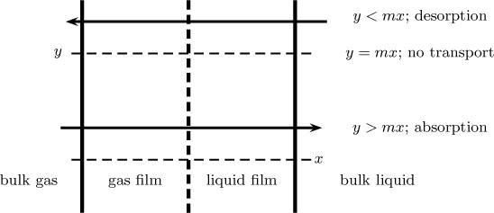
Diagrammatic representation of the absorption and desorption for calculation of driving forces.

Figure 6.8 Driving force calculations for absorption and desorption. The difference y – x is not the correct driving force.

Controlling Resistance

It is also important to know which film offers the major resistance to mass transfer. This depends on the controlling resistance, which may be on the gas side or the liquid side depending on the value of H_A.

If H_A is a small number which corresponds to a highly soluble gas, then the controlling resistance is on the gas film and K_G ≈ k_G.

If H_A is a larger large number which corresponds to poorly soluble gas, then the controlling resistance is on the liquid film and K_L ≈ k_L.

Similarly, if m is large (low solubility case), then the liquid-side resistance is controlling and K_x ≈ k_x. The reverse is true for small m. In that case, K_y ≈ k_y. The calculation of the overall resistance is illustrated in Example 6.9.

Example 6.9 Calculation of the Overall Coefficient

SO₂ is absorbed into water in a packed column. At a point in the column the bulk conditions are y_A = 0.1 and x_A = 0.01. The Henry’s law constant is 440 atm. Temperature is 300 K and the total pressure is 5 atm. The mass transfer coefficients are k_G = 4 × 10^–5 mol/m²s atm and k_L = 2 × 10^–4 m/s. Find the rate of absorption at this point. Calculate and sketch the concentration profiles in the gas and liquid films.

Solution: The units of the Henry’s law constant suggest that the equilibrium is represented as p_A = Hx_A, with A being the solute SO₂. For the problem, p_A = 0.1 × 5 = 0.5 atm. This sets the gas-phase value.

The liquid concentration is 0.01 and hence the equilibrium partial pressure is $p_{A}^{*}$ $p_{A}^{*}$ = 0.01 × 440 = 4.4 atm. The overall driving force is 0.5 – 0.44 = 0.06 atm.

The overall mass transfer coefficient is calculated from Equation 6.52. A note of caution is that the Henry constant for this equation should be in pressure-concentration units. Hence the given value of 440 atm is converted by dividing it by the total liquid concentration. The corresponding flux value is obtained by multiplying this by the overall driving force.

The overall coefficient turns out to be nearly the same the as gas side coefficient indicating that all the resistance is on the gas side. The result for the flux ix then 2.4 × 10^–6 mole/m².

Summary

Stagnant systems are defined as systems with no superimposed external flow. They may not always be truly stagnant, as a flow can be generated in such cases due to diffusion itself. A common example is evaporation of a liquid in an inert gas. The evaporation causes a flow (often barely noticeable), which then enhances the rate of transport. The enhancement is often accounted by a drift flux correction factor.
An Arnold cell is a simple device to measure the diffusion coefficient (in gas mixtures) by simple measurement of the change in the level of a liquid due to evaporation. The model for such systems is based on the concept of a pseudo-steady state. The evaporation is calculated as though the system were in (pseudo-) steady state at any given instant of time. The liquid level is then obtained as a function of time using the pseudo-steady state value for the evaporation.
The assumption of a pseudo-steady state is used in many problems in mass transfer calculations. This assumption is reasonable whenever the time scale of diffusion is much smaller than the process time.
Mass transfer near a fluid–solid interface is often modeled by using a film model. This model assumes there is a stagnant film near the interface within which all the resistance to mass transfer is contained. The diffusional rate of transport can then be calculated using the relation D/δ_f (or equivalently a mass transfer coefficient) multiplied by the overall concentration difference.
The film model is very useful to study mass transfer accompanied by a surface reaction. For a simple first-order reaction with no mole change, an overall rate constant can be defined and used. The reciprocal of this rate constant is the sum of the reciprocal of the mass transfer coefficient and the reciprocal of the reaction rate constant. Thus it is not the true or intrinsic rate constant, but merely a convenient parameter for representing the data. The methodology is exactly equivalent to the law of addition of resistances.
The simple concept of resistances fails even for a first-order reaction when there is a change in the number of moles present due to reaction. The counter-diffusion of the product can enhance or retard the mass transfer rate. For nonlinear kinetics, even with no change in moles, the resistance concept does not hold. In such a case, a nonlinear or transcendental implicit equation for the rate is generally obtained.
The film model when applied to a fluid–fluid (gas–liquid or liquid–liquid) systems necessitates the use of two films—one on the gas side of the interface and the other on the liquid side. Each film offers its own resistance to mass transfer. These resistances can be added (for the low flux mass transfer case) to get an expression for the overall resistance. Correspondingly, an overall mass transfer coefficient can be defined and used to calculate the mass transfer rate.
The mass transfer rate may be governed by the gas-side resistance, the liquid-side resistance, or both. Relative contributions can be evaluated, which is a very useful information for selection of appropriate equipment and design.
For a highly soluble gas, the resistance is mostly in the gas film; the reverse is true for a poorly soluble gas.

Review Questions

6.1 What is meant by the determinacy condition? Why is it needed?

6.2 What is meant by UMD and EMD? Which factors are different in mass transfer calculations for each of these?

6.3 What is meant by the drift flux correction factor? Where is it used?

6.4 State the assumptions involved in the film theory of mass transfer.

6.5 What is the relationship between film thickness and the mass transfer coefficient?

6.6 State the difference between film thickness in the film model and the concentration boundary layer thickness in the convection–diffusion model.

6.7 If the mass transfer coefficient is measured at a low concentration of a solute, how would you correct it for high concentration? Assume UMD.

6.8 A surface reaction follows first-order kinetics. What is the unit of the rate constant?

6.9 A surface reaction follows second-order kinetics. What is the unit of the rate constant?

6.10 Distinguish between the apparent rate constant and the true rate constant.

6.11 A heterogeneous reaction is taking place under a rapid reaction condition. State the equation to calculate the flux to the surface and the rate of reaction.

6.12 What is the relation between K_G and K_L?

6.13 What is the Schmidt number? What is its role in boundary layer theory and mass transfer calculations?

Problems

6.1 Variable diffusivity example. A spherical capsule has an outer membrane thickness with inner and outer radii r_i and r_o, respectively. A solute is diffusing across this capsule. Consider the case where the diffusion coefficient is a function of concentration and can be represented in a general form as D(C_A); it is not a constant. Derive an expression for the (total) rate of mass transport across this spherical shell. Use the low flux model.

6.2 Evaporation from a beaker. Benzene is contained in an open beaker that is 6 cm high and filled to within 0.5 cm of the top. Temperature is 298 K and the total pressure is 1 atm. The vapor pressure of benzene is 0.131 atm at these conditions and the diffusion coefficient is 9.05 × 10^–6 m²/s. Find the rate of evaporation based on the low flux model, the exact model, and the low flux model corrected by drift flux.

6.3 Level change calculation. For problem 2, find the time for the benzene level to fall by 2 cm. The specific gravity of benzene is 0.874. For this condition (H = 0.5 + 2 cm), find the mole fraction profile of benzene in the vapor phase and compare it with the linear approximation (which would be the prediction of the low flux model).

6.4 Mass transfer across two bulbs. Two bulbs are connected by a straight tube of 0.001 m in diameter and 0.15 m in length. Initially the first bulb contains nitrogen and the second bulb at the other end contains hydrogen. The system is maintained at a temperature of 298 K and a total pressure of 1 atm. The volume of each bulb is 8 × 10^–6 m³. Calculate and plot the mole fraction profile of nitrogen in bulb 1 as a function of time.

6.5 Mass transfer with first-order surface reaction. Species A is diffusing to a catalytic surface, where it undergoes a first-order surface reaction. Equal moles of product counter-diffuse from the catalytic surface to the bulk gas. A rate of 1.6 × 10^–4 mol/m²s was measured when the system was at 2 atm pressure and temperature of 300 K, with 10% A in the bulk gas. The mass transfer coefficient was estimated for the given flow conditions as 2 × 10^–4 m/s. Estimate the true rate constant. If the gas velocity is doubled, find the rate of reaction. Assume that the mass transfer coefficient changes with gas velocity to the power of 0.8.

6.6 Mass transfer with second-order surface reaction. Species A is diffusing to a catalytic surface, where it undergoes a second-order surface reaction. Equal moles of product counter-diffuse from the catalytic surface to the bulk gas. A rate of 8 × 10^–4 mol/m² s was measured when the system was at 2 atm pressure and a temperature of 300 K, with 10% A in the bulk gas. The mass transfer coefficient from the bulk gas to the catalyst was estimated for the given flow conditions 2 × 10^–4 m/s. Estimate the true rate constant.

6.7 Effect of product counter-diffusion. An example of a problem in which a severe counter-diffusion of the products takes place is the deposition of SiO₂ from tetraethoxysilane (TEOS) on a solid substrate. The reaction is represented as

SiO(C₂H₅)₄(g) → SiO₂(s) + 4C₂H₄(g) + 2H₂O(g)

Note that 6 moles have to counter-diffuse, which retards mass transfer unless the mole fraction of TEOS is small. Consider deposition from a gas at temperature of 400 K and 0.1 atm pressure, with a mole fraction of TEOS of 0.2. Diffusivity is 0.1 cm²/s and the film thickness is 2 mm. Calculate the rate of reaction (equal to the rate of diffusion to the surface) and the film growth rate, assuming that the surface reaction is very rapid.

6.8 Effect of stoichimetry on mass transfer rate. In a combustion chamber, oxygen diffuses through air to a carbon surface, where it reacts. Depending on the reaction surface conditions and temperature, either CO or CO₂, or a mixture of both, is produced. The reaction at the surface can be assumed to be rapid. The conditions are mole fraction of oxygen in the bulk gas is 0.21; pressure = 2 bar, temperature = 600 K. The film model with a film thickness of 1 mm can be used for mass transfer, and the diffusion coefficient of oxygen in the system has a value of 0.2 cm²/s. Calculate the rate of reaction assuming that only CO₂ is produced as the product. Calculate the rate of reaction assuming that only CO is produced as the product.

6.9 Shrinking rate of a reactive particle. Uranium solid is reacted with fluorine to produce a gas-phase precursor of uranium according to the reaction

U(s) + 3F₂(g) → UF₆(g)

What is the expression for the combined flux of F₂ (denoted as species A here) in this system? If fluorine diffuses to an uranium surface through a film of thickness , derive the expression for the flux of fluorine to the surface. Assume the bulk mole fraction is y_Ab and the mole fraction at the slab surface is zero.

Now consider that the reaction is taking place on a solid sphere of radius R, and the transport of F₂ from the bulk gas to the surface through a thin boundary layer near the solid surface is the rate-controlling step. Again assume the bulk mole fraction is y_Ab and the mole fraction at the slab surface is zero. Also assume that the gas is stagnant. Derive an expression for the rate of fluorine transferred to the sphere $(M_{A})$ $(M_{A})$ .

6.10 Series reaction in a nonporous catalyst. Consider a nonporous catalyst with a series reaction occurring at the surface:

A → B → C

Derive equations for the rates of reaction of A and B considering diffusional resistances. Use a low flux model.

6.11 Various definitions of mass transfer coefficient. At a certain point in an absorber, the value of k_y is 7 × 10^–3 kmol/m²s and that of k_x is 2 × 10^–4 kmol/m²s. The system has properties similar to air and water and is at 300 K and 1 atm. Find k_G, k_m, and k_L.

6.12 Driving force and overall mass transfer coefficient. At a certain point in a mass transfer system, the bulk mole fractions are y_A = 0.04 in the gas phase and x_A = 0.004 in the liquid phase. The mass density of the liquid is nearly the same as water. The Henry’s law constant for A is reported as 7.7 × 10^–4 atm m³/g mol. Determine whether the species absorbing or desorbing. If the mass transfer coefficients are k_G = 0.010 g mol/m² s atm and k_x = 1.0 (mol/s m²), find the overall transfer rate. Here k_x is the mass transfer coefficient on the liquid side based on the mole fraction difference as the driving force. Find the percentage of the resistance in each film.

6.13 Overall mass transfer coefficient. In an absorption column, the following parameters were observed: liquid-side mass transfer coefficient = 4 × 10^–4 m/s; gas-side mass transfer coefficient = 2 × 10^–4 gmol/m²s atm. The Henry’s law coefficient is 100 atm expressed as p = Hx. Find the overall mass transfer coefficient for the system K_L. Also state the relative percentage contribution of the resistances on the gas side and the liquid side.

6.14 Contribution of gas-side resistance. The value of k_G in an absorber is 3 × 10^–3 kmol/m²s atm and k_L is 5.44 × 10^–3 m/s. Find the contribution of the gas side for Henry’s law coefficients of 0.1, 1, and 10 m³ atm/kmol.

..................Content has been hidden....................

You can't read the all page of ebook, please click here login for view all page.

Table of Contents for Chapter 6. Diffusion-Dominated Processes and the Film Model

Create new playlist

Sign In

Sign Up

Chapter 6. Diffusion-Dominated Processes and the Film Model

6.1 Steady State Diffusion: No Reaction

6.1.1 Combined Flux Equation

6.1.2 Diffusion-Induced Convection

6.1.3 Determinacy Condition

Nt versus nt

6.1.4 Low Flux Model: The Laplace Equation

6.2 Diffusion-Induced Convection

6.2.1 Conditions for the Validity of the Low Flux Model

6.2.2 Analysis for UMD

6.2.3 Drift Flux Correction Factor

6.2.4 Mole Fraction Profiles in UMD

6.3 Film Concept in Mass Transfer Analysis

6.3.1 Boundary Layer Concept for Fluid–Solid Mass Transfer

Results from Boundary Layer Theory for a Flat Plate

Relation to Momentum Boundary Layer

Why Use the Film Model?

6.3.2 Film Model Approximation

6.3.3 Film Model: Determinacy Correction Factor

6.4 Surface Reactions: Role of Mass Transfer

6.4.1 Low Flux Model: First-Order Reaction

Measured versus True Kinetics

6.4.2 Low Flux Model: Nonlinear Reactions

Second-Order Reaction

Bimolecular Reaction

6.4.3 High Flux Model: Effect of Product Counter-Diffusion

Fast Reaction

Slow Reaction

6.5 Gas–Liquid Interface: Two-Film Model

6.5.1 Mass Transfer Coefficients

Gas Side

Liquid Side

6.5.2 Overall Mass Transfer Coefficient

Gas-Phase Driving Force

Liquid-Phase Driving Force

Mole Fraction Driving Force

Determining the Direction of Transfer

Controlling Resistance

Summary

Review Questions

Problems

Table of Contents for
Chapter 6. Diffusion-Dominated Processes and the Film Model

N_t versus n_t