
Chapter 20. Gas–Liquid Reactions: Film Theory Models
Learning Objectives
After completing this chapter, you will be able to:
Model systems where a gas is absorbed into a reacting liquid based on the film model.
Understand the role of a key dimensionless parameter, the Hatta number, in determining the extent of reaction in the film (fast reactions) relative to that in the bulk liquid (slow reactions).
Distinguish the various regimes of absorption for a fast reaction and examine the effect of operating parameters for these cases.
Extend and study the modeling of more complex systems by taking an example of simultaneous absorption of two gases.
Couple the film model with macro- or meso-models for the reactors in order to set up design equations for the absorber or stripper.
Understand the role of dissolving and reacting fine particles in enhancing the rate of gas–liquid mass transport.
Gas–liquid reactions are common in industrial chemical production and in gas purification processes. Examples in chemical production can be found in liquid phase oxidation reactions such as production of cyclohexanol by oxidation of cyclohexane, p-xylene oxidation to produce terephthalic acid, chlorination of liquid benzene, and so on. Additional important examples can be found in gas purification processes and environmental cleaning, including CO2 removal from various gas streams such as natural gas, synthesis gas, SO2 removal from refinery gases and so on. In gas purification, the amount of gas that can be removed by physical absorption is limited due to equilibrium considerations. The rate can be enhanced significantly by absorbing in a reactive liquid. Carbon dioxide removal by absorbing into amine solutions is one such example.
In general gas absorption in a reacting liquid involves mass transfer from gas to liquid followed by reaction in the liquid phase. The goal of this chapter is to use the fundamentals of mass transfer and to calculate the rate of absorption for a wide range of process conditions.
Mass transfer analysis is done on the basis of the film model here. Note that the film model postulates the existence of a stagnant film near the gas– liquid interface. For fast reactions, species A (dissolved gas) may react in this film itself and simultaneous diffusion and reaction considerations are needed for this. If the reactions are slow, however, the mass transfer and reaction occur in series and the model is simpler. Hence we first show the criteria to distinguish the two, the extent of film reaction versus bulk reaction. The analysis is based on a first-order reaction of the dissolved gas.
The variation of the concentration of the second reactant, that is, the liquid phase reactant, is another consideration and depending on some parameter values, it may deplete in the film thereby affecting the rate of reaction in the film. The no depletion case is shown first. Then we show how the rate of absorption may be predicted if depletion occurs. The analysis for multiple reactions or simultaneous absorption of two gases is then shown, mainly using numerical tools.
Gas–liquid reactor level models are set up by coupling the local rate of mass transfer predicted by the film model to a meso- or macro-model for the equipment. Examples are shown to illustrate how the two levels are coupled and these will provide an introduction to set up reactor level models. A brief section is also provided for the case of mass transfer in a gas–liquid–dissolving solid system.
The discussions and the theoretical underpinnings also apply with some modifications to a liquid–liquid reaction and a brief section on this is also provided together with the pertinent references.
Gas absorption systems can also be modeled based on the penetration model for mass transfer rather than the film model. This involves the solution of the transient diffusion with reaction model. This is presented in Chapter 21, which can be studied together with the current chapter.
20.1 First-Order Reaction of Dissolved Gas
Consider a gas A that dissolves into a liquid and undergoes a first-order reaction in the liquid phase. We analyze the process based on the film model. The concentration profiles envisioned in the film model are shown schematically in Figure 20.1.

Figure 20.1 Schematic of the film model and the concentration profile of the dissolving and reacting gas in the liquid film. The dashed line represents the case of no reaction in the film.
The steps shown in Figure 20.1 are the following. Gas A diffuses from the bulk gas to the interface through the gas film, dissolves into the liquid at the interface, undergoes simultaneous diffusion and reaction in the liquid film, and crosses over the bulk liquid. Dissolved A can further react in the bulk liquid. There is no concentration profile in the bulk liquid that is assumed to be uniformly mixed. The dashed line in Figure 20.1 represents the concentration profile if no reaction occurred in the film.
The governing equation for species in the film is the diffusion-reaction equation:
The solution of this gives the concentration profile and the flux of A at the interface and into the bulk liquid. The reaction rate is assumed to be first order in A with a rate constant k1, which has units of s–1.
20.1.1 Boundary Conditions
The boundary conditions used for this problem are the following:
A simple Dirichlet condition is used at the interface. At where (equilibrium at the interface). This is valid if there is no appreciable resistance on the gas side of the interface. Then pAi is nearly the same as the (known) bulk gas partial pressure of A, denoted in Figure 20.1 as pAG.
If there is significant gas-side resistance as well, then the model has to be coupled with gas-side transport and a Robin boundary condition has to be used at the interface. Note that the flux balance in the gas film gives the following relation between the bulk gas and the interfacial partial pressures:
Here kG is the gas-side mass transfer coefficient. This can be used to set pAi in an iterative manner.
At x = δ (the edge of the film thickness) CA = CAb, which is the dissolved concentration of gas A in the bulk. The bulk concentration of A cannot be independently assigned. The calculation of the dissolved gas concentration in the bulk involves coupling of the film model with a macroscopic model for the bulk liquid. (A Robin boundary condition can be derived rather than the Dirichlet used here.) This is explained in Section 20.2. We use a fixed value here for bulk concentration in order to focus on what is happening in the liquid film. Also, it may be noted that the bulk concentration often approaches zero if the process in the bulk liquid consumes the dissolved gas at a reasonably fast pace. In that case, the bulk liquid balance for dissolved A is not needed.
20.1.2 Dimensionless Version
The dimensionless form is obtained by defining a dimensionless concentration and a dimensionless distance ξ = x/δ:
The dimensionless parameter appearing in the model is named the Hatta number squared. This is defined as
Note that this has the same grouping of quantities as the Thiele modulus squared, introduced in the context of reactions in porous catalysts. Also note that the film thickness is often not known. What is generally known is the liquid side mass transfer coefficient kL. The film thickness can be estimated from this parameter since kL = DA/δ. Hence an alternative representation of Hatta number is
It can be shown that the Hatta number squared is a measure of the relative rate of reaction to diffusion or the ratio of the time scale for diffusion in the film to the time scale of reaction. Thus a large Hatta number implies a fast reaction and correspondingly a significant drop in the concentration of A in the film.
The boundary conditions in dimensionless form are cA(ξ = 0) = 1 (no gas-side resistance case) and cA(ξ = 1) = cAb, the dimensionless bulk concentration of A. The solution for the concentration profile with these boundary conditions is
You may wish to verify the mathematical detail leading to this.
20.1.3 Flux Values at the Interface and into the Bulk
Flux at the interface is obtained by using Fick’s law at the interface:
Using the expression for the concentration profile the interfacial flux is given as
Note that the flux is not proportional to C*A – CAb, unlike the case of physical absorption. The above result was first derived by Hatta (1932).
The quantity of dissolved gas going into bulk is computed from the flux at the edge of the film (δ) (i.e., use Fick’s law at this point) and the resulting expression is
Where Does the Reaction Occur? Film or Bulk
In most cases the concentration in the bulk can be set to zero when Ha > 1. Only in exceptional cases where the volume of the film is comparable to the total volume of the liquid would there be a finite dissolved concentration in the bulk liquid when Ha > 1. The value of CAb can in general be estimated by a mass balance for the bulk liquid. Hence it is appropriate to take CAb as zero for further discussion and examine where the reaction is taking place.
A useful quantity is fractional extent of reaction in film:
This is the measure of how much of the reaction occurs right when A is diffusing across the film. (This expression is obtained by combining Equations 20.6 and 20.7.)
The following values can be calculated for illustration:
If Ha = 0.2, then the fractional extent of reaction in the film is only 1.97%. Note that CAb may not be zero in these cases and an estimation of this value is given in the next subsection.
If Ha = 1 then the fractional extent of reaction in the film is about 0.3519. The assumption that CAb = 0 is adequate here in most cases and for larger values of Ha.
If Ha = 3 the fractional extent of reaction in the film is nearly 90%.
If Ha = 5 the fractional extent of reaction in the film is nearly 98.6%.
If Ha = 10 all reaction is in the film itself. Nothing reaches the bulk.
A plot of the concentration profile for various values of Ha is shown in Figure 20.2. The plot is in agreement with the discussion on the fractional extent of reaction in the film as well.

Figure 20.2 Concentration profiles for A in the film where it undergoes a first-order reaction. Note the slopes at ξ of 0 and 1, which is the measure of the local fluxes at these points and are representative of mass crossing the interface and moving into the bulk, respectively.
20.1.4 Enhancement Factor
The flux at the interface is also a measure of the quantity of gas absorbed per unit interfacial area per unit time and is expressed as dimensionless flux, which is also known as the enhancement factor, E. This is defined as
This is a measure of the gas absorbed from the liquid in a reacting case compared to a non-reacting case. Using the earlier expression for NA0, we have:
Note that this expression assumes CAb to be zero.
Following simplified expressions for the enhancement factor for a fast reaction is useful and widely used in many applications. The fast reaction case applies if Ha > 3. All the reaction takes place in the film for a fast reaction. For Ha > 3, the tanh Ha term can be approximated as one. Hence E = Ha.
Using this in the definition of E, the following expression is obtained for the flux of A at the interface:
Note that δ cancels out and the film thickness no longer matters; the rate of absorption does not depend on δ and kL, the value of the mass transfer coefficient.
Correspondingly, the volumetric rate of absorption is given as
It depends only the gas–liquid interfacial area. The measured volumetric rate of absorption can be then used to estimate the interfacial area under these conditions, a technique widely used in many studies. (This presumes that the values for DA and k1 are known from independent measurements.)
20.2 Bulk Concentration and Bulk Reactions
We now look at how the dissolved concentration of A in the bulk liquid may be estimated and the extent to which the bulk reaction takes place. The bulk composition is determined by a mass balance for the bulk liquid. The control volume can be either a meso- or macroscopic element of the bulk liquid (depending on the extent of mixing in the liquid). An illustrative control volume for the analysis presented here is shown in Figure 20.3.

Figure 20.3 Control volume (solid rectangle) and the terms needed for the mass balance in the bulk liquid.
20.2.1 Bulk Concentration
The concentration of dissolved gas in bulk can be calculated starting from a mass balance over this control volume:
In crossing at the edge of the film at δ + in from adjacent bulk control volume – out into adjacent control volume = consumed in bulk + accumulation.
For batch systems where there is no flow in or out of the bulk, it may be appropriate to simplify the balance as
In at δ = Consumed in the bulk.
Here we also neglect accumulation and focus on any instant of time where the input term balances the reaction. This is equivalent to assuming that the bulk liquid is at a pseudo-steady state at a given instant of time.
In at δ, the edge of the film, is given by Equation 20.7. We multiply NAδ by the gas–liquid interfacial area agl to get the volumetric transfer rate. Hence
This balances the reaction in the bulk, which is given as
Here
∊′L = ∊L – δagl
This represents the volume of the bulk liquid per unit reactor volume. Note that this is often approximated as ∊L since the thickness of the film is usually very small.
The value of CAb can now be obtained by solving Equations 20.10 and 20.11 simultaneously. The volumetric absorption rate in turn is obtained by using this value of CAb in any one of these equations. The additional parameter needed in this model is ∊′L/δagl.
The dimensionless bulk concentration is shown in Figure 20.4 as a function of Hatta number for two values of the ∊′L/δagl parameter. The bulk concentration is nearly zero if Ha > 0.6.

Figure 20.4 The bulk concentration values for a batch absorber as a function of Hatta number for two values of the volume ratio parameter.
20.2.2 Absorption Rate Calculation for Ha < 0.2
If Ha < 0.2 most of the reaction occurs in the bulk and the film reaction can be neglected. The expression for CAb can be simplified for this case and a correspondingly simpler expression for the volumetric rate of absorption can be obtained, which is presented in this section.
We note here for Ha < 0.2, the cosh(Ha) term will be nearly one and the sinh Ha and tanh Ha terms are nearly equal to Ha. Hence Equation 20.10 simplifies. Combining the resulting expression with Equation 20.11 leads to the following result for the bulk concentration.
Correspondingly the expression for the rate of absorption simplifies to
This can also be expressed in the two resistance form by taking the reciprocal on both sides:
Two limiting cases of this expression will now be examined.
The first is the case of a kinetically limited reaction. The condition for this to be applicable is k1∊L << kLagl, that is, the reaction rate is smaller than the mass transfer rate and the reaction rate is rate limiting. The liquid will remain at the saturation concentration:
The reaction rate is simply governed by the kinetics of the reaction. The bulk concentration of A will be now the same as the saturation concentration of the gas.
The second is the mass transfer limited reaction; the condition for this to be applicable is k1∊′L >> kLagl, that is, the reaction rate is much larger than the mass transfer rate. Mass transfer from interface to bulk liquid is rate limiting. The bulk liquid concentration is nearly zero due to the rapid rate of mass transfer. The rate of absorption now becomes
The rate is controlled by the rate at which A arrives from the interface to the bulk liquid. The bulk concentration is nearly zero for this case. The two cases are sketched in Figure 20.5.

Figure 20.5 Kinetically controlled and mass transfer controlled cases. Concentration in the bulk liquid compared to the interfacial concentration for a case of no reaction in the film.
A brief summary of the various regimes of absorption are as follows. Given the data on the rate constant and diffusion coefficient, the mass transfer coefficient should be independently measured or estimated. This permits us to calculate Ha and see if the reaction is mainly in the film or mainly in the bulk. The following regimes can then be identified depending on the magnitude of Ha:
Ha > 3: Reaction occurs entirely in film. The rate of absorption depends only on the gas–liquid interfacial area for a first-order or pseudo-first-order reaction. The intrinsic mass transfer coefficient does not play a role.
0.5 < Ha < 3: For this range some reaction occurs in film and some in bulk. But the bulk balance leads to a nearly zero concentration of A in the bulk and this assumption can be used to simplify the rate calculation.
Ha < 0.5: No reaction occurs in the film. Two subcases can be noted now depending on the relative values of k1∊′L and kLagl:
– k1∊′L >> kLagl: Mass transfer to bulk is rate controlling. The rate of absorption depends on the volumetric mass transfer coefficient. The bulk concentration will be nearly zero here.
– k1∊′L << kLagl: The chemical reaction is rate limiting. The rate of absorption does not depend on the mass transfer coefficient. It depends on the rate constant and the liquid holdup. Bulk concentration is nearly equal to saturation solubility under these conditions.
20.3 Bimolecular Reactions
In this section we consider the case where the reaction is first order in both gases A and B. The reaction scheme considered is a bimolecular reaction, represented as
A(g → l) + νB(l) → Products
Examples of such a system include CO2 absorption in various reacting solvents such as amine solutions and many other gas treating processes. We consider a case where some or most reactions are taking place in the film and examine the effect of transport of B from the bulk liquid to the interface. The diffusion-reaction differential equation is now applied to both species A and B.
The governing equations are as follows:
Here x is the actual distance into the film with x = 0 representing the gas–liquid interface.
20.3.1 Dimensionless Representation
We now introduce the relevant dimensionless parameters. The dimensionless concentration that will be used is
cA = CA/C*A
C*A is the equilibrium solubility of gas A in the liquid corresponding to the partial pressure of A at the gas phase:
C*A = pAG/HA
Here HA is the Henry’s law constant for species A in units of atm m3/mol. Note the definition and the unit since there are many ways of defining the Henry constant.
Similarly the dimensionless concentration for B is defined as
cB = CB/CBL
where CBL is the bulk liquid concentration of B.
Finally ξ is used for the dimensional distance in the film and defined as = x/δ.
With these variables, the governing equations are the following:
and
Two dimensionless quantities appear in the dimensionless formulation. These are
and
Noting that kL = DA/δ, the Hatta number can also be expressed as
The Hatta number (squared) represents the ratio of diffusion time to reaction time and hence a large drop in concentration in the film can be expected for large values of this number. The q parameter is the measure of the concentration ratio of B to A. A relatively large drop in concentration of B in the film can be expected if this parameter is small.
Boundary Conditions
The boundary conditions for species A are as follows. At the interface, the boundary condition will depend on whether the gas film resistance is included or not and will be of the Dirichlet or Robin type. The two cases are as follows:
Case 1: No gas film resistance. Here at ξ = 0, CA = C*A and Hence cA = 1. The boundary condition is now of the Dirichlet type.
Case 2: Gas film resistance included. A balance over the gas film provides the boundary condition:
Also note that pAi, the interfacial partial pressure of A, is related to the interfacial concentration of A in the liquid by Henry’s law. Thus CA(x = 0) = pAi/HA. Using these, the boundary condition at ξ = 0 can be expressed in dimensionless form as
where BiG = kGHA/kL, a Biot type of number for gas–side mass transfer. The boundary condition is now of the Robin type.
At ξ = 1, the edge of the film, CA = CAb is some specified value depending on the bulk processes. This value CAb will depend on the extent of bulk reactions, convective and dispersive flow into the bulk and so on, similar to the model in Section 20.2.1. But even for moderately fast reactions, the bulk concentration of dissolved gas turns out be zero and we take this value to be zero. Hence cA = 0 at ξ = 1 will be used as the second boundary condition. The validity of this assumption can be checked after a solution is obtained by a bulk balance for A and modified if needed.
The boundary condition for species B are specified as follows. At ξ = 0 we use dcB/dξ = 0 since B is non-volatile and the flux is therefore zero. At ξ = 1, we have cB = 1. This completes the problem definition.
The results are generally presented in terms of an enhancement factor E, defined as
This is a measure of the flux at the interface. Here we use p for the concentration gradient dcA/dξ.
Since the profiles of A and B are now coupled this calls for a numerical solution. We will study the numerical solution using a MATLAB solver in a later section. But the essential details of the concentration profiles that can be expected are shown in Figure 20.6.

Figure 20.6 Concentration profiles in the film for a gas–liquid reaction, showing three regimes of absorption. Gas film resistance is not included here.
Rather than solving numerically we present here various limiting cases that gives us a feel for the problem and the results that could be anticipated from the MATLAB solution. Three regimes can be classified and analytical solutions can be obtained for these cases. These regimes are pseudo-first order, second order, and instantaneous. The regimes depend on the interfacial concentration of B and this is first estimated in the following section.
20.3.2 Invariance Property of the System
A relation between the concentration profiles of A and B exists purely based on the stoichometry of the reaction; this is known as the invariance property and is derived in this section.
The rate terms can be eliminated between Equation 20.17 and Equation 20.18 to give
This can be integrated once to give
Here the integration constant has been assigned as the dimensionless concentration gradient of A at the interface. We note that the no flux boundary condition for B at the interface is satisfied by this choice for the constant.
A second integration and use of boundary condition at ξ = 1 gives
cA = qcB + p0ξ + A1
From the boundary conditions at ξ = 1, we can show that A1 = –p0 – q. Hence the concentration profile of B is related to that for A as
This is the invariant property that ties together the A and B concentrations.
The important quantity is the interfacial concentration of B, denoted as cBi, as it determines which of the previuosly indicated regimes are likely to exist. This is obtained readily by setting ξ = 0 in the above expression: this is an invariant of the system. All numerical results should show this result; otherwise the numerical procedure is wrong.
Since the enhancement factor E is equal to –p0, the resulting invariant equation is written in terms of E as
The three regimes are now classified as follows:
Pseudo-first-order reaction: This occurs when cBi is nearly equal to one. Analysis for this case is similar to that in Section 20.1 and is presented in Section 20.3.3.
Instantaneous reaction: This occurs when cBi is nearly equal to zero. Analysis for this case is presented in Section 20.3.4.
Second-order reaction: The interfacial concentration of B is quite lower than one but does not approach zero. This is also known as the depletion regime. Analysis for this case is presented in Section 20.3.5.
It may be worthwhile to estimate the conditions where cBi is nearly unity. This will happen if E << q. But we do not know E. Let us proceed further assuming that the interfacial concentration of B is nearly unity. In this case Equation 4.18 can be solved analytically. We call this a pseudo-first-order model.
20.3.3 Analysis for Pseudo-First-Order Case
In this case cBi = 1 and cB in Equation 20.18 can be set to one. The differential equation for A is now linear and analytic solution for CA obtained in 20.1 for a first-order reaction is applicable. The corresponding enhancement factor derived in Section 20.1.4 is applicable. Hence:
Using this value of E in Equation 20.26 we find that if Ha << q then the concentration of B will be nearly one at the interface, leading to a pseudo-first-order approximation. Hence the condition for the applicabiity of the pseudo-first-order reaction is that Ha << q.
The following results are of importance when the reaction occurs under pseudo-first-order conditions:
The volumetric rate of absorption depends only on the gas–liquid interfacial area and not on the composite parameter kLagl.
The observed dependency on the concentration of B is half order although the reaction is intrinsically first order in B.
20.3.4 Analysis for Instantaneous Asymptote
The second limit can be analyzed easily as well. There are two ways of doing this. The first is that mathematically we set cBi = 0 in Equation 20.26. We find
One can show that if Ha >> q, the instantaneous asymptote is reached, while if Ha < q, the pseudo-first-order regime will be observed.
The second approach is based on a physical consideration that postulates that there is a reaction plane λ that separates the A and B regions. In other words we assume that A and B cannot co-exist in the film. The physical situation prevailing is shown in Figure 20.6 earlier in the chapter.
The rate of absorption and reaction is controlled by the rate of transport A from the interface to the reaction plane:
This is balanced by the rate of transport of B from the bulk to the reaction plane which is
Equating these two expressions for NA0 one can solve for both λ and NA0, Based on NA0 the enhancement factor can be calculated. The result is the same as Equation 20.28.
The approximation E = q is commonly used in Equation 20.28 since q is usually large (roughly 10 or so). In such case the volumetric rate of absorption is given as
Usually CBL is larger than C*A and the first term is dropped. Then
This is a rather interesting result that states that the rate is not a function of the gas concentration.
20.3.5 Second-Order Case: An Approximate Solution
For Ha ≈ q a second-order reaction case is reached where both equations (profiles for A and B) have to be solved together. This can be done numerically. However, a good analytical approximation was proposed by Hikita and Asai (1963). They claimed that the pseudo-first-order asymptote can still be used provided the Ha parameter is now based on the interfacial concentration of B rather than the bulk concentration. The rationale for doing this is that species A reacts in a zone near the interface and the concentration seen by A is mostly equal to CBi. The fact that CB varies in the film is not of much significance as far as the rate at which it reacts. Thus RA local = k2CBiCA is good enough. We thus can still use Equation 20.27 but with a modified Hatta defined as
This leads to the following expression for E:
where cBi is given by Equation 20.26. Note that cBi is a function of E and hence we have to solve for both E and cBi simultaneously. Simple MATLAB code to do this is given in Listing 20.1. The enhancement factor is calculated given the two dimensionless groups Ha and q. A third group BiG is also to be considered if there is appreciable resistance on the gas film. The code also includes the effect of this parameter on cBi.
Listing 20.1 Enhancement Factor for Second-Order Reaction
% Hikita-Asai model solver. Hikita2.m
% Dimensionless parameters
Q = 50.; HA =50.00; Bi_G = 100.;
% Case 1: No gas side resistance case
Bi_fun = @(X) (1.0 + 1./Q -HA * X^0.5 *coth(HA * X^0.5) /Q - X );
bi0= 0.008 % trial value
bi = fsolve (Bi_fun, bi0)
E1 = HA * bi^0.5 * coth(HA * bi^0.5)
% Case 2: With gas side resistance
Bi_fun = @(X) (1.0 + 1./Q -HA * X^0.5 *coth(HA * X^0.5) /Q ...
*(1.+ 1./Bi_G) /(1+HA * X^0.5* coth(HA * X^0.5)/Bi_G) - X );
bi = fsolve (Bi_fun, bi0)
E = HA * bi^0.5 * coth(HA * bi^0.5)/ ...
(1. + HA * bi^0.5 * coth(HA * bi^0.5)/Bi_G)
An example of calculation of the interfacial concentration of B and the enhancement factor is shown next in Example 20.1.
Example 20.1 Effect of Ha on the Interfacial Concentration
Using Listing 20.1 show the effect of Ha on cBi and E for a fixed value of q = 50. Also show the effect of gas film resistance for Ha = 5.
Solution
If Ha = 5 running the code we get an interfacial concentration of 0.9239 and a corresponding enhancement factor E of 4.806, which is close to a pseudo-first-order reaction.
If Ha = 50, we find the interfacial concentration of B is 0.3931 and the corresponding enhancement factor is 31.3471. The regime is second order and appreciable depletion of B in the film occurs.
If Ha = 500 we get a cBi that is close to zero and hence the instantaneous regime is approached. The enhancement factor is 50.49, which is close to instantaneous value of 51.
Thus by increase of Ha, the regime of absoprtion shifts from pseudo-first order to second order and finally to instantaneous.
The above results are in the absence of gas film resistance for illustration of the regime change.
If gas-side resistance were included with BiG = 10, Ha = 50, and q = 50, we find the following results: the interfacial concentration of B is 0.4945 and the corresponding enhancement factor is 26.01. The interfacial concentration is higher but the enhancement factor is lower since there is some concentration drop of A in the gas film.
An illustrative application to carbon dioxide absorption in sodium hydroxide solution is presented next in Example 20.2.
Example 20.2 CO2 Removal with NaOH Solution
Carbon dioxide is absorbed into a solution of NaOH in a packed column absorber. Locally at a given point in the absorber the concentration of NaOH is 1.0 M and the partial pressure of CO2 is 1 atm. Find the rate of absorption. Neglect the effect of gas-side resistance. Parameters needed are shown as part of the solution.
Solution
The physico-chemical parameters needed are listed below together with the values specific to this problem. The parameter values are taken from the work of Danckwerts (1960). Solubility of CO2 at 1 atm pressure = 30 mol/m3.
Diffusivity of gas A (CO2) and liquid reactant B (NaOH) are DA = 1.8 × 10⁻⁹ m2s and DB = 1.7DA. The rate constant for the reaction is k2 = 10 m3/mole.s
The hydrodynamic parameter needed is the liquid-side mass transfer coefficient. We use kL = 1 × 10⁻⁴ m/s for illustration. Gas-side resistance is neglected here.
The dimensionless parameters Ha and q are first calculated from Equations 20.21 and 20.20 and the values are found to be 42 and 21.25, respectively.
The next step is to solve Equations 20.26 and 20.29 simultaneously for the interfacial concentration of B and the E value. We find cBi = 0.186. Hence this represents a condition where there is a significant depletion of the reactant at the interface.
The enhancement factor is calculated as 18.3. Correspondingly the rate of absorption is kLC*AE and is equal to 0.0539 mol/m2 s.
20.3.6 Instantaneous Case: Effect of Gas Film Resistance
The regime of instantaneous absorption is often accompanied by considerable gas film resistance. In some cases, the process can become entirely limited by the gas-side resistance and the reaction plane shifts to the interface. The reaction of the gas then takes place directly at the interface. This section examines the effect of gas film resistance for an instantaneous reaction and the conditions when the reaction plane will shift to the interface.
The concentration profile for an instantaneous reaction including the drop in concentration in the gas film is shown in Figure 20.7. Also shown are three possible cases that are discussed in the following.
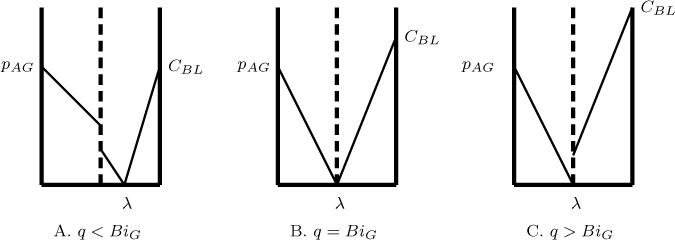
Figure 20.7 Concentration profiles of A and B for an instantaneous reaction with gas film resistance included; note the shift in controlling regime.
The analysis starts with various transport steps and the corresponding rate equation. For the gas film transport of A we use
The transport of A from the interface to a distance λ is given as
Finally from the transport consideration for B from the bulk liquid to the interface we have
We now have three equations for three unknowns: NA0, pAi, and λ. The final result can be expressed in terms of the enhancement factor, now defined as
It is easier to solve for E, if the various expressions are in term of 1/E. From the transport equations of A (gas film plus 0 to λ) we can show that 1 E =
Here BiG is the Biot number defined as kGHA/kL.
From the transport considerations for B we find
where q is now defined as DBCBL/(νDApAg/HA).
Equating the two expressions for 1/E and solving for λ we obtain
It should be noted here that this equation is valid only if q < BiG since λ cannot be negative. (The lambda has to be positive or at the most can be equal to zero. If it is zero, the reaction plane would be right at the interface.) In such case the value of E is simply equal to BiG; the process becomes controlled entirely by gas film resistance.
Using this value λ in either of the equations we find the enhancement factor (for the case where q < BiG) can be calculated after some “minor” algebra as
and for q > BiG as
It is useful to illustrate the calculations to a numerical problem, which we do in Example 20.3.
Example 20.3 H2S Absorption in NaOH Solution
Hydrogen sulfide absorption in amine solutions may be assumed to be instantaneous. At a point in the absorber the total pressure is 20 atm and the gas contains 1% H2S. The ratio DB/DA is 0.64 and the amine concentration is 0.25 M. The mass transfer coefficients are kL = 0.01 cm/s and kG = 2 × 10⁻⁵ mol/cm2 s atm. The Henry’s law constant for H2S is 1950 Pa m3/mol.
Find the rate of absorption at this point. Also find the amine concentration when the process becomes entirely controlled by gas-side mass transfer.
Solution
We need two dimensionless numbers, q and BiG, to use the model for instantaneous reaction with gas-side resistance. It is useful to convert the Henry’s law constant to atm to simplify the calculations. The value is 1950/1 × 105 = 0.0195 atm m3/mole.
The required parameters are calculated as
The enhancement factor is then calculated as (1 + q)/(1 + 1/BiG) and is equal to 16.18.
The rate of absorption is calculated as kL(pAG/HA) × E and is found to be 0.0166 mol/m2.s.
If the concentration of amine is increased the rate is increased and reaches a case where it becomes gas-side controlled. This concentration is reached when q = BiG. The concentration is found to be 625 mol/m3. The rate of absorption at this point is calculated as kGpAG and is equal to 0.04 mol/m2.s. If the amine concentration is increased further, the rate stays at this point since the reaction plane has already shifted to the interface. These are useful guidelines for choosing the optimum operating conditions depending on the mass transfer coefficient prevailing in the contactor, which is discussed briefly next.
20.3.7 Choice of Contactor Based on the Regimes of Absorption
The contactor to be used depends on the regime. Thus in a pseudo-first-order scenario, a contactor that develops a large interfacial area is important. For a slow reaction, a large volume of liquid is needed and intense agitation to create a large interfacial area is not needed. For the instantaneous case the overall mass transfer coefficient is important and contactors that provide this are needed.
20.4 Simultaneous Absorption of Two Gases
In this section, we analyze a case where two gases dissolve simultaneously and react with a common liquid phase reactant. Many complex reaction schemes can be analyzed using a similar approach and hence it is useful to study this example. Simple CHEBFUN-based code is also given for the two gas absorption case (Listing 20.2) and the code can be modified and used for many other applications.
The reaction scheme considered in this section is represented as
A + νAC → Products
B + νBC → Products
where A and B are the two gases being absorbed and C is the common liquid phase reactant.
Each reaction is assumed to be second order overall (1,1 order) kinetics with rate constants of kA and kB for the first and second reaction.
20.4.1 Model Equations
Governing equations follow from the diffusion-reaction model and are as follows:
Boundary conditions at x = 0 are
CA = C*A; CB = C*B; dCC/dx = 0
The gas-side resistance is not included here but can be added by incorporating a Biot number dependency and changing the gas A and B boundary conditions at x = 0 to a Robin condition.
Boundary conditions at x = δ for a fast reaction that consumes A and B in the bulk are
CA = 0; CB = 0; CC = CCL
In general a bulk balance is needed to estimate the bulk concentrations of the dissolved gas similar to single gas absorption. These refinements are also not addressed here in order to focus on the ramifications of the film diffusion-reaction part of the model.
20.4.2 Dimensionless Representation
We now introduce the following dimensionless parameters: distance in the film ξ = x/δ; concentrations of the gaseous species: cA = CA/C*A and cB = CB/C*B; concentration of the liquid phase reactant cC = CC/CCL.
The dimensionless forms are then obtained and are as follows:
and
The dimensionless quantities needed are as follows
The boundary conditions are
At ξ = 0: cA = 1; cB = 1; dcC/dξ = 0
At ξ = 1: cA = 0; cB = 0; cC = 1
20.4.3 CHEBFUN Solution
The solution was implemented numerically using CHEBFUN in MATLAB, and the code is presented in Listing 20.2. This code is illustrative of two gases being absorbed but can be modified easily for other cases of mass transfer accompanied by complex reactions. (See paper by Ramachandran and Sharma (1971) for many examples of absorption of gases followed by complex reactions).
Listing 20.2 Code for Simulation of Absorption of Two Gases with Reaction in the Film
%% Simultaneous gas absorption with fast second–order reaction
% parameters
MA = 1.E+04; qa =0.1 ; MB = 10.0; qb = 0.2;
% declarations
x = chebfun ('x', [0,1])
a = chebfun ('a', [0,1])
b = chebfun ('b', [0,1])
c = chebfun ('c', [0,1])
N = chebop (0,1)
N.op = @(x,a,b,c)[ diff(a,2)–MA*a.*c , ...
diff(b,2)–MB*b.*c , ...
diff(c,2)–qa*MA*a.*c–qb*MB*b.*c ]
N.lbc = @(a,b,c)[ a–1,b–1,diff(c) ];
N.rbc = @(a,b,c) [ a, b, c–1]
% N.guess = [0*x,0*x];
sol = N�
diffsol = diff(sol) % derivative of the solution
% trial solution for the next case
N.guess = sol(:,:)
plot(sol)
xlabel ( 'Dimensionless distance in the film ' )
ylabel ( ' dimensionless concentrations ' )
fluxA = –diffsol(0,1)
fluxB = –diffsol(0,2)
..
Illustrative results are shown in Figure 20.8 for a chosen set of parameters.

Figure 20.8 Concentration profiles for A, B, and C in the film for simultaneous absorption of two gases; the parameters used are MA = 100, MB = 5, qA = 10, qB = 5.
Note that A drops very fast near the interface and the instantaneous reaction condition is nearly approached. B reacts near δ and some of B goes into the bulk and reacts there as well. The bulk conditions are assumed to be such that the concentration of B is zero. The enhancement factor for B is now 1.440. If gas A were not present then the factor would be 2.66. The program enables us to calculate the rate of absorption as a function of various parameters. Normally this will be put as a submodel at film scale in the overall reactor model.
20.5 Coupling with Reactor Models
Some examples are shown here where we couple the film model with the reactor model. These examples provide a clear illustration of how the local differential model for rate of transfer is incorporated into a larger scale reactor or equipment model. The approach is the same as that for physical absorption and models for reacting systems are extensions with the reaction terms added to the macro- or meso-balances. For example the model for a packed bed gas– liquid reactor is developed on similar lines to that in Section 4.3.2.
20.5.1 Semibatch Reactor
A common mode of operation is a semibatch reactor where a gas containing a solute A is bubbled into a pool of agitated liquid where it (A) dissolves and reacts with a species present in the liquid phase. The schematic is the same as in Figure 3.3 where we considered absorption of oxygen in a non-reacting pool of liquid. The model is set up using species conservation laws applied to A in the gas phase, dissolved A in the bulk liquid, and liquid phase reactant B. The mass transfer model provides the expression for the rate terms at any instant of time. A general formulation should include the film and bulk reaction and is shown in this section. Simplifications can be made appropriately when one of the processes is more dominant. The mass balance equations follow. The following equation applies for the concentration of the dissolved gas in the bulk liquid:
The liquid phase reactant concentration is given by
Here NBδ is the flux of B into the film. This represents the B needed to satisfy the stoichiometry for the reaction of A occurring in the film. This is given as
This equation states that the B reacted in the film is the difference in the flux of A at the interphase and that to the bulk. The film model gives the values for these quantities, NA0 and NAδ. It is solved at each point in time and these values are updated during the time marching scheme.
The representative concentration to be used for the gas phase needs some additional consideration. Two cases need to be distinguished depending on the level of mixing in the gas phase and modeled accordingly.
1. Gas is backmixed: The representative concentration to be used here is the exit gas concentration. This needs to calculated by a gas phase balance, which is represented in the following equation:
Expressing NA0 in term of the enhancement factor E, which is in turn a function of yAe and CBL, the gas phase mass balance becomes
The inert balance is used to relate Ge to Gi. Since there is no net change in the inert gas flow rate we have
Using this in Equation 20.51 we obtain
This gives a quadratic equation for yAe and the solution gives the representative concentration to find the interface concentration and rate of absorption.
The enhancement factor depends on the value of yAe and CBL at the current value of time. This is solved in a separate subroutine, for example, using the Hikita-Asai model (for example, using Listing 20.1).
2. Gas is in plug flow: The gas phase balance is a differential balance for this mixing pattern:
This is solved simultaneously with the liquid phase balance to find the exit concentration of the gas. The representative concentration is the log mean of the inlet and the exit concentration.
The model is general and is applicable for the intermediate case where reaction can occur in both the film and the bulk. Simplified models can be used for fast reactions as discussed in the following.
Fast Reactions
For fast reactions the dissolved gas concentration in the bulk is not needed. This simplification is allowed because all reactions are in the film and therefore NAδ = 0.
The liquid phase reactant concentration can also be simplified as
where C*A = yAeP/HA is the saturation solubility. This is applicable if the gas is well mixed. If the gas is in plug flow the log mean mole fraction of A should be used to find the saturation solubility.
Note that E in Equation 20.50 is a function of the current value of the liquid phase composition and not a constant. Thus
E = E(CBL) = f(Ha, q, BiG)
where Ha and q are based on the values at the current time. This variation should be included in the integration procedure and E should not be treated as a constant.
Levenspiel suggests tabulating the value of E as a function of CBL and then using a graphical integration using a rearranged form of Equation 20.55. Thus a formal solution for batch time tB to achieve a required conversion is
However it is easier to do this computationally using time marching. Using the simple first-order explicit finite difference for the time derivative in Equation 20.55 we have the following scheme for the simulation:
Here an explicit Euler scheme is used, which is sufficiently accurate. The time step has to be chosen such that the concentration changes only by 5% to 10% at each time step.
The computational scheme is therefore as follows for a semibatch liquid with a well-mixed gas phase.
Use the condition at t where we know CBL. Calculate Ha.
Assume yAe. This sets the q parameter and is calculated next.
Using Ha and q, estimate E.
Use E to update yAe using Equation 20.51 until convergence is obtained. Both of these calculations can be done together using the FSOLVE routine in MATLAB, where both E and yAe are solved simultaneously.
Update CBL to time t + Δt by using a finite difference version, Equation 20.56, and continue time marching.
The computational scheme for the case where the gas is in plug flow is similar. The representative concentration to be used in the calculation of the enhancement factor is now the log mean average value. A differential balance is now used for the gas phase instead of Equation 20.51. The liquid phase balance remains the same (Equation 20.55) with the difference that E is now based on the log-mean gas mole fraction. The computational procedure is similar to that for the backmixed case. Step 4 of the computational step is modified and the gas concentration profile is estimated by solving the plug flow equation at the current time.
20.5.2 Packed Column Absorber
Packed column absorbers are usually modeled by assuming plug flow for both phases. Bulk gas concentration is generally zero if Ha > 1. Reactions may occur in the film or the bulk liquid but if the bulk gas concentration is zero, the bulk liquid balance for A is not needed.
Model equations where the concentration of A in the bulk liquid is zero are presented in the following.
For species A the material balance is
Here Ac is the area of cross-section of the column. It is more convenient to write material balance equation in terms of the enhancement factor:
The molar flow rate of gas can vary in the column for concentrated gas mixture and an equation for its variation is obtained by an inert balance:
Hence
For dilute systems the 1 – yA term can be approximated as one and hence
The liquid phase balance for reactant B for countercurrent flow is
Equations 20.61 and 20.62 are now solved simultaneously as a boundary value problem. At each step the value for E should be calculated based on the local bulk gas and bulk liquid conditions:
E = E(yA, CBL)
A MATLAB-based simulation scheme can be set up for this but the details are not presented here due to space limitations.
20.6 Absorption in Slurries
Gas absorption with chemical reaction in slurries is encountered in a large class of industrially important processes, such as gas treating, pollution control, oxidation, chlorination, hydrogenation, and so on. Examples of such systems can also be found in the field of product engineering, for instance, in making products such as calcium carbonate, magnetic particles such as geothite, and so on. A particularly important case arises when a gas is absorbed in a slurry containing fine particles (where the particle size is smaller than the diffusion film thickness). The particles then modify the concentration profile in the film thus affecting directly the rate of mass transfer.
Ramachandran and Sharma (1969) provided a starting point in this field which has led to many further works in both modeling and applications. A brief overview is provided here on how fine particles present in the film can enhance the rate of mass transfer. The comprehensive review of the development and more details are summarized by Ramachandran 1993.
The system analyzed here is that of a gas dissolving into a slurry of liquid + solid particles. The slurry consists of soluble particles that dissolve in the liquid and react with the dissolved gas. The reaction scheme can be represented by the following scheme:
A(g) → A(aq)
B(s) → B(aq)
A(aq) + B(aq) → Products
An example is absorption of CO2 in a slurry containing Ca(OH)2 particles.
20.6.1 Particle Size Effect
Two cases can be distinguished depending on the relative size of the diffusion film and the particle:
Large diameter particles (compared to film thickness) such that the particle concentration in the film is small. Here the dissolution takes place in the bulk of the liquid. The dissolved species B diffuses toward the film and reacts with A and the reaction is often complete in the film itself for fast reactions. The enhancement in the gas absorption is only due to the homogeneous reactions taking place in the film and can be calculated by the models described in Section 20.2. The criteria for this regime to hold was derived as
Particle size is smaller than the film thickness. These are referred to as fine particles or more generally as “microphase.” Here the solid dissolution occurs in parallel to the reaction taking place in the film. The rate of gas absorption is enhanced above that calculated from the pure gas–liquid reaction theory.
The conceptual basis for the enhancement of the mass transfer rate due to the presence of fine particles is shown in Figure 20.9.

Figure 20.9 A general schematic of the effect of suspended particles on the concentration profiles in the liquid film. The dotted line is for the case of absence of the particles while the solid line is for the particles present in the film.
The concentration profiles for species A and B are shown in the presence (solid lines) and absence of particles (dotted lines) in the film. The simultaneous dissolution of B in the film contributes additional liquid phase reactant and makes the concentration profile of A steeper. An additional enhancement in the the rate of absorption follows as a consequece. Since the rate of absorption is proportional to the concentration gradient at the interface, we find that rate is enhanced in the presence of the fine particles dissolving in the film. The extent of depletion of B in the film is also reduced, which contributes further to the increase in the rate.
For many systems of industrial importance (such as SO2 in lime slurry), the reaction itself can be treated as instantaneous and hence this case is treated here based on the film model.
20.6.2 Instantaneous Reaction Case
The concentration profiles for species A and B for an instantaneous reaction are presented in Figures 20.10.

Figure 20.10 Schematic profiles for A and B for an instantaneous reaction case; λ is the location of the reaction plane. The dotted line denotes a case of no particles while the solid line represents the presence of particles.
Since the reaction is instantaneous, we have a reaction plane at x = λ where the reaction occurs. The location of the reaction plane is closer to the interface in the presence of solids as shown by the solid line. The dotted line shows the case where the solid dissolution in the film is negligible. In either case for an instantaneous reaction, we have a A-only region from 0 to λ and a B-only region from λ to δ.
For the B-only region, λ to δ, the following equation holds for species B:
The CBS is the saturation solubility of the species B. The previous equation can be expressed in terms of dimensionless variables as
Here βsf is a dimensionless group that characterizes the solid dissolution in the film and is defined as
It represents the square root of the ratio of the time scale for film diffusion to the solid–liquid mass transfer.
For small particles, a limiting value of ksl = DB/R can be used since the Sherwood number, ShR, for solid–liquid mass transfer is equal to one in the limiting case of a stagnant particle. In addition, asl = 3∊s/R. Hence βsf can also be expressed as
Hence the range of values for βsf depends on the particle size, R, and particle loading, ∊s, and is on the order of 0 to 4 for many practical systems.
For the A-only region, 0 to λ, the following equation holds for the concentration distribution of species A, assuming that the particle dissolution rate is equal to the local rate of reaction:
This can be expressed in terms of dimensionless variables as
where the concentration ratio parameter q is defined as
The quantity of interest is usually the rate of absorption, RA, which is defined more conveniently in terms of an enhancement factor, E, given as
The position of the reaction plane is obtained by a flux balance at the reaction plane:
or in terms of dimensionless variable as
Solution of Equations 20.69 and 20.65 yields the concentration profiles from which the gradients can be calculated and used in Equations 20.71 and 20.73. The final results are as follows:
For the enhancement factor we obtain
and for the (dimensionless) reaction plane we have
In the limiting case of large q, the value of E can be shown to be equal to qβsf . Using Equation 20.67 for βsf and 20.70 for q, the following expression for the rate of absorption is obtained in the limiting case:
NA0 becomes inversely proportional to the particle size and directly proportional to the square root of the particle loading, which has also been confirmed in some experimental studies.
20.7 Liquid–Liquid Reactions
Liquid–liquid reactions provide another example where mass transfer effects are important and need to be included in the analysis. In such systems, due to mutual solubility, the reaction can occur in one or the other phase or in both phases. This is unlike a gas–liquid reaction where (for most cases) there is no reaction in the gas phase. The film model is again useful to visualize the processes and to develop a mathematical model.
Examples of liquid–liquid reactions are shown in Table 20.1.
Table 20.1 Some Examples of Liquid–Liquid Reactions
Reaction – |
Phase I organic |
Phase II aqueous |
nitration |
benzene |
nitric acid |
hydrolysis |
alkyl acetate |
NaOH |
alkylation |
butane |
isobutylene |
eserification |
fatty acids |
methanol |
polymerization |
trimesolyl chloride |
diamine |
desulfurization |
organic sulfur |
peroxyacetic acid |
The concentration profile according to the film model is shown for two components A and B reacting with each other in Figure 20.11.

Figure 20.11 Two-film model representation of a liquid–liquid reaction between A and B. The solid line is the profile of A and the dotted line is the profile of B.
The film model is developed by proceeding with a formulation similar to that given in Section 20.2. The differential equations for the two components for both phases are used, leading to four differential equations. The equilibrium conditions (concentration jump) are used as an interfacial boundary condition together with the flux continuity condition at the interface. In some cases analytical solutions are obtained.
The reactor level models are then developed by coupling the local models with the macroscopic or mesoscopic models for the two phases depending on the mixing pattern in each of the phases. Vasudevan and Sharma (1984) have studied the modeling of common types of liquid–liquid reactors.
Summary
Gas–liquid reactions are another important area with many applications where mass transfer analysis is needed and effectively used to understand and design such systems. The film model is often used as the basis for modeling these systems.
The basic model where gas A dissolves and undergoes a first-order reaction should be studied carefully. Two regimes can be identified depending on the magnitude of a key dimensionless parameter, the Hatta number. The Hatta number is a measure of relative rate of reaction to diffusion. Large Hatta numbers lead to a reaction being confined to a thin region near the gas–liquid interface. Small Hatta numbers lead to species A crossing the film without appreciable reaction and then reacting in the bulk of the liquid.
The mass transfer rate is enhanced due to reaction, especially for Ha > 1, the film reaction case. An enhancement factor is defined and used to characterize this enhancement. For large Ha and a first-order or pseudo-first-order reaction, this enhancement factor turns out to be equal to Ha. The volumetric rate of reaction is then dependent on only the gas–liquid interfacial area under these circumstances and is not dependent on the intrinsic mass transfer coefficient kL.
For small Ha most of the reaction takes place in the bulk liquid. A bulk liquid balance is then used to find the dissolved gas concentration in the bulk liquid. Correspondingly, two regimes can be identified for this case: a mass transfer controlled case where the bulk concentration is nearly zero, and a reaction controlled case where the bulk is almost at the saturation solubility of the gas.
The identification of the controlling regime is important for making the correct choice of the equipment to be used. If the reaction is mostly in bulk, then equipment with large bulk volume is used. If the reaction is in film, thin film contactors may be sufficient since the bulk volume is not being utilized in this case.
The liquid phase reactant concentration should also be modeled for bimolecular reactions. For an appreciable extent of the reaction in the film, species B concentration can deplete in the film and in some cases the reactions can become instantaneous, in which case the species B concentration falls to zero in a region near the gas–liquid interface. The model proposed by Hikita-Asai is useful to estimate the level of depletion (the interfacial concentration of B) and to use this to calculate the enhancement factor by an approximate analytical solution.
Depending on the concentration of B at the interface three regimes can be identified, which are sketched in Figure 20.6. These are B concentration nearly the same as bulk, leading to a pseudo-first-order model; moderate depletion of B, leading to the second-order model; and complete depletion, leading to the instantaneous reaction model. The relative magnitude of Ha and q determines the extent of depletion.
For a pseudo-first-order case, the rate turns out to be square root dependency on B concentration, even though the reaction is intrinsically first order on B. The rate is also proportional to the square root of the rate constant.
For an instantaneous reaction the rate of absorption is solely determined by mass transfer considerations, that is, how fast the reactant can reach the reaction plane. The chemical kinetics plays no role under these conditions. The rate is observed to be strongly dependent on the B concentration and not affected significantly by gas concentration.
The gas-side resistance can be included in the differential model for dissolved gas transport as a Robin condition. An additional parameter, the Biot number for gas-side mass transfer is needed. The boundary condition at the interface is switched to a Robin condition using this parameter.
Simultaneous absorption of two gases with a common liquid phase reactant is an industrially important problem in gas treating and also an example of absorption with multistep reactions. Hence it is important to understand the methodology of model development for such reactions. For the particular scenario examined, we find the rate of absoprtion of gas B is severely affected by the presence of gas A due to the fast reaction of A with C, thereby making C unavailable to react with B in the regions near the interface.
Two examples of coupling the film model with the reactor model were illustrated in the text. The mixing pattern of the phases need to be assumed and macroscale or mesoscale model for the reactor scale need to be set up. The local rate of absorption (film model) is then incorporated as a submodel in the reactor model.
Absorption in a liquid containing dissolving particles is of importance in many applications. Fine particles can dissolve in the film itself, raising the local concentration of B, and thereby enhancing the rate of gas absorption, providing additional enhancement in absorption. For larger particles the dissolution is mainly in the bulk and the gas–liquid models directly apply since the solid dissolution and reaction occur in series rather than simultaneously.
Models for liquid–liquid reactions follow a similar pattern to gas–liquid reactions. The reactions can now take place in one or both phases depending on the relative solubility of the reactants. The general procedure is to set up the diffusion-reaction model for one or both phases and solve these equations. Reactions can in some cases take place at the interface itself for very fast reactions and when the solubility of one component in the other phase is limited. This is similar to a gas–liquid instantaneous reaction shifting to the interface.
Review Questions
20.1 What is the physical significance of the Hatta number?
20.2 Express Hatta (squared) as a ratio of two time constants.
20.3 How can the extent of reaction taking place in the liquid film be calculated?
20.4 State some approximate condition when the bulk liquid concentration can be approximated as zero.
20.5 Explain on physical grounds why the absorption rate is not dependent on the film thickness for a first-order reaction if Ha > 3.
20.6 State conditions when the volumetric rate of reaction does not depend on the value of the intrinsic mass transfer coefficient.
20.7 What is the bulk liquid concentration for a purely kinetic controlled reaction?
20.8 State the three dimensionless parameters needed to model a bimolecular gas–liquid reaction.
20.9 What is meant by the invariance property of a system?
20.10 How can you calculate the interface concentration of the liquid phase reactant B?
20.11 State conditions when the reaction may be assumed to be instantaneous.
20.12 State conditions when the reaction may be assumed to be pseudo-first order.
20.13 Compare the effect of concentration of B on the observed rate of absorption if the reaction is under pseudo-first order conditions versus if the reaction is instantaneous.
20.14 When does an instantaneous reaction become completely controlled by the rate of gas-side mass transfer?
20.15 What is the difference in mass transfer mechanism if a gas is absorbed in a slurry with fine particles versus that with large particles?
Problems
20.1 Flux expressions for absorption with a first-order reaction. Verify the details leading to Equations 20.6, 20.7, and 20.8.
20.2 Gas absorption in an agitated tank with a first-order reaction. Oxygen is absorbed in a reducing solution where it undergoes a first-order reaction with a rate constant of 6 s–1. The conditions are such that the liquid-side mass transfer coefficient kL is equal to 8 × 10⁻³ cm/s. Will there be appreciable reaction in the film? Use DA = 1.5 × 10⁻⁵ cm2/s for dissolved oxygen. What would be rate of absorption/reaction if the oxygen partial pressure in the gas phase is 0.21 atm? Use the same Henry constant as that for oxygen in water. Neglect the bulk concentration of dissolved oxygen. Also find the flux of O2 going into the bulk liquid and calculate the percentage of O2 that reacts in the film itself.
20.3 Carbon dioxide absorption with first-order reaction. CO2 is absorbed into a liquid under conditions such that the liquid-side mass transfer coefficient is 2 × 10⁻⁴ m/s. The diffusion coefficient of CO2 in the liquid is 2 × 10⁻⁹ m2/s. The interfacial concentration of CO2 can be found using Henry’s law. The pressure is 1 atm and the temperature is 300 K. Assume that CO2 reacts with a dissolved solute in the liquid with a rate constant of 1 s–1. Also assume that the bulk concentration of CO2 is zero. Find the Hatta number. Find the flux of CO2 at the interface. Find the flux of CO2 going into the bulk liquid. What percentage of CO2 reacts in the film itself?
20.4 Gas absorption with a bimolecular second-order reaction. Carbon dioxide is absorbed into a solution of NaOH in a packed column absorber. Locally at a given point in the absorber the concentration of NaOH is 1.0 M (1000 mol/m3) and the partial pressure of CO2 is 1 atm. The parameters needed are listed as follows: Henry’s law constant = 1500 bar (in p = Hx form); diffusivity of gas A (CO2) and liquid reactant B (NaOH) are DA = 1.8 × 10⁻⁹ m2/s, DB = 1.7DA; rate constant for the reaction k2 = 10 m3/mole.s; liquid-side mass transfer coefficient kL = 1 × 10⁻⁴ m/s. Neglect gas-side resistance. Find the dimensionless parameters Ha and q. Compare these values and indicate what regime applies for gas absorption. Find the rate of absorption per unit interfacial area. If the interfacial area is 200 m–1 find the volumetric rate of gas absorption.
20.5 Change in regime due to partial pressure and concentration changes. For the previous problem, examine the effects of changing (1) the partial pressure of CO2 and (2) the concentration of liquid phase reactant. State the range of conditions where the reaction is expected to be under pseudo-first-order conditions. State the conditions under which the reaction can be treated as instantaneous. Note that the following rough rules apply: the reaction can be treated as pseudo-first order if Ha < q/5, and the reaction can be treated as instantaneous if Ha > 5q.
20.6 Absorption with instantaneous reaction. Hydrogen sulfide absorption in amine solutions may be assumed to be instantaneous. At a point in the absorber the total pressure is 20 atm and the gas contains 2% H2S. The ratio DB/DA is 0.64. The mass transfer coefficients are kL = 0.03cm/s and kG = 6 × 10⁻⁵ mol/cm2s.atm The Henry’s law constant for H2S is 1000 Pa m3/mol. Find the rate of absorption for amine concentrations in the range of 0.25 to 1.5 M. Also plot the location of the reaction plane as a function of the amine concentration.
20.7 Lo-cat process for hydrogen sulfide removal. In this process hydrogen sulfide bearing gas is absorbed in a chelated iron Fe+3 solution where it undergoes a reduction to form elemental sulfur:
H2S + 2Fe+3 → 2Fe++ + 2H+ + S
At a certain point in the reactor the partial pressure of H2S is 5% and the chelate concentration is 60 mol/m3: Find the rate of absorption given the following data: Henry′s law constant = 1950 Pa m3/mol; diffusivity of gas A(H2S) = 1.44 × 10⁻⁹ m2/s; diffusivity of liquid reactant: DB = 0.54 × 10⁻⁹ m2/s, rate constant for the reaction k2 = 9 m3/mole.s; liquid-side mass transfer coefficient kL = 2 × 10⁻⁴ m/s; gas-side mass transfer coefficient kG = 2 × 10⁻⁴ mol/Pa m2s; gas liquid transfer area = 200 m–1.
20.8 Absorption with a reversible reaction. Consider a simple reversible reaction:
A ⇌ P
–RA (local) = k1(CA – CP /K) where K is the equilibrium constant for the reaction. Use the following boundary conditions. At the interface CA = C*A and there is no flux for P (P is non-volatile). At the bulk CA = CAb and CP = KCAb, that is, bulk liquid composition is at equilibrium. Set up the models and solve the equations. Derive an expression for the enhancement factor. Hint: P concentration can be expressed in terms of A concentration, thereby reducing the model to a single differential equation for A only.
20.9 Ozone absorption with reaction. Wastewater is contacted with an ozone containing gas in a CSTR. The gas phase ozone concentration is 3% and the gas volumetric flow rate is 3 cu.m/sec. Find the extent of consumption of ozone in water and in the exit gas composition. The parameters needed are as follows. The diffusion coefficient is 2 × 10⁻⁹ m2/s. The rate constant (first-order reaction) 4 s–1. The process is liquid-side mass transfer controlled with a coefficient of 4 × 10⁻⁴ m/s. The interfacial area is 200 m2/m3.
20.10 Simultaneous absorption of two gases with one gas reacting instantaneously. An example of this is in simultaneous absorption of H2S and CO2 in amine solution. The reaction of H2S is instantaneous and hence there is a C-depleted zone near the interface of thickness λ. This thickness is also to be determined as part of the solution.
For the region 0 to λ there is no C. Show that the following equations hold:
and
For the region λ to δ there is no A and the following equations hold:
and
State the boundary conditions needed to solve the problem. State the additional conditions needed to find λ. Set up the model in dimensionless form and find the effect of the presence of A on the rate of absorption of B and vice versa.
20.11 Simulation of a batch absorber with reaction. Gas A is bubbled into an agitated liquid containing a liquid phase reactant B. Find the time needed to reduce the concentration of B starting from 5000 to 500 mol/m3. Use following parameters for transport parameters: kL = 2 × 10⁻⁴ m/s; agl = 100 m2/m3 of dispersion volume; DA = 2 × 10⁻⁹ m2/s; also use DB = DA; stoichiometric coefficient ν = 2. Values of physico-chemical parameters at the operating temperature of 300 K are as follows: Henry constant: 1000 m3Pa/mol; rate constant k2 = 10 m3/mol.s, assuming a (1,1) order reaction. The operating pressure is 1 atm.
20.12 Simulation of a packed column. A gas stream containing 2.3% chlorine at a molar velocity of 100 mol/m2s is treated with NaOH solution that is flowing countercurrent to the gas at the rate of 250 mol/m2s. The concentration of NaOH in the feed liquid is 2736 mol/m3. The reaction is instantaneous and the other parameters are H = 125 × 106 atm m3/mol, kGagl = 133 mol/m3 hr atm, and kLagl = 45 hr–1. Find the height of the tower needed to achieve 90% removal of chlorine.
20.13 Absorption in slurries with fine particles. Calculate the enhancement due to the presence of the particles for the following case: Particle size = 10 μm; C*A = 4 mol/m3; CBs = 20 mol/m3; DA = 2 × 10⁻⁹ m2/s; DB = 2 × 10⁻⁹ m2/s; ν = 1; kL = 1 × 10⁻⁴ m/s. Particle loading is 10%. The reaction is assumed to be instantaneous.
20.14 Liquid–liquid reaction. Biodiesel are methyl esters of fatty acids and are produced by reacting triglycerides (TG) with methanol (ME). The reaction scheme is represented as
T G + 3ME → E + G
where G is the side product, glycerol. The reaction is (2,1) order and the rate constant is 1.2 × 10⁻⁴ C2T CM . The solubility of triglycedride in methanol is represented as CT (methanol phase) = 25CT (oil phase). The mass transfer coefficient of TG into methanol is 3 × 10⁻⁵ m/s. The reaction was carried out in a microchannel flow reactor with two phase flowing concurrently into the reactor. The reactor diameter used was 0.5 mm and the length was 2.5 m. A mole ratio of 6 to 1 for oil to methanol was used. The flow rate of was 2.92 ml/min TG and 0.57 for ME and the interfacial area for mass transfer was 30,000 m2/m3. Simulate the reactor and estimate the exit concentrations of TG and M.