
Chapter 23. Biomedical Applications
Learning Objectives
After completing this chapter, you will be able to:
Explain the role of mass transfer in biomedical systems.
State and use the Hill equation for oxygen-hemoglobin equilibrium.
Model oxygen transport in lungs and calculate the oxygen profile in an alveolar capillary.
Understand the Krogh model for oxygen transport in tissues and identify the oxygen starved region.
Develop pharmacokinetic models to predict drug metabolism.
Set up and solve a mesoscopic model for a dialysis system and link it to model a patient-hemodialyzer system.
Mass transfer principles find important applications in biomedical engineering. For a biomedical engineer a mechanistic understanding of processes such as oxygen transport in lungs and tissues is important per se and also in evaluating medical conditions and adjusting the treatment protocols. For pharmacokinetic scientists who deal with the study of distribution of a drug and its metabolism in the body, the modeling of mass exchange between various compartments/organs is the main tool needed. For the design of many extra-corporal devices, for example, dialysis, membrane oxygenators, artificial liver, and so on, it is necessary to evaluate the role of transport in the equipment and adjust the operating conditions accordingly. Hence we note that modeling of these systems where mass transport plays a key role is an important component of biomedical engineering. The goal of this chapter is to take some of these examples, illustrate how fundamental transport considerations are useful to model, and analyze these processes.
The analysis presented in this chapter is at a simplified level, making some assumptions but nevertheless providing important information and indicating the main factors affecting the process. Upon studying this chapter you will be able to see how the concepts learned in Part I of the book can be applied to prototypical biomedical problems. This broadens your skill in applying mass transfer principles to a wider class of problems than in traditional chemical engineering.
Transport of gaseous species (in dissolved form) is encountered in a number of organs and is shown schematically in Figure 23.1. Two main mass transfer steps are oxygen exchange in lung to blood and oxygen transfer from blood to tissues. Mass transfer–based models to describe these are discussed in Sections 23.1 and 23.2 respectively. Analysis of distribution of drugs together with their metabolism can be modeled by the compartmental models that were introduced in Section 13.8. Additional information and some more detailed modeling trends are then shown in Section 23.3. Modeling of extracorporal devices is illustrated by a mesoscopic-based model for a hemodialyzer in Section 23.4. Here we also show how this model can be linked to a compartment model to simulate the patient blood concentration during a dialysis treatment.

Figure 23.1 Overview of oxygen and carbon dioxide mass transfer in human body. Based on Silverthorn D. U, (2001). Human Physiology, An Integrated Approach, Second Edition. Prentice Hall, 2nd ed, Upper Saddle River, N.J.
23.1 Oxygen Uptake in Lungs
In this section we consider the modeling of oxygen uptake in lungs (Exchange II in Figure 23.1). First we consider the equilibrium concentration that can be reached in blood for the reaction of oxygen and hemoglobin (abbreviated as Hb). Then we enumerate the transport steps and derive an expression for local transport at any point. This is then included in a mesoscale model for the capillary to calculate the oxygen concentration versus length along the alveolar capillary. One can clearly see the similarity with the mass exchanger modeling studied in earlier chapters.
23.1.1 Oxygen-Hemoglobin Equilibrium
A simple way to calculate equilibrium concentration in blood in contact with air is to apply the law of mass action to the reaction of oxygen and Hb:
O2 + Hb ⇄ O2Hb
Using the law of mass action, we obtain
where the square bracket shows the concentration. K is the equilibrium constant for the reaction.
Using Henry’s law [O2] = pO2/HO2. Let S be the fraction of Hb existing in oxygenated form. Then [O2Hb] = CT S and [Hb] = (1 – S)CT where CT is the total concentration of Hb in oxygenated plus free form. Using these in the law of mass action, we have
Solving for S, we get
The above model based on a single reaction scheme does not fit the actual data, which shows an S-shaped curve as shown in Figure 23.2. This is ascribed to oxygen binding to more than one site in a cooperative manner. There are four heme groups in Hb. Binding of oxygen to the first heme group facilitates binding to subsequent sites, resulting in the S-shaped curve shown in Figure 23.2.

The equilibrium curve is therefore fitted as
This is referred to as Hill’s equation. The equation is often written as
Here p50 is the partial pressure at which the oxygen saturation is 50%.
The exponent should be four if oxygen binds consecutively to the four sites. The data, however, fits with an exponent of 2.7. The value of p50 is 26 mm Hg.
For oxygen binding to myoglobin (a carrier found in muscles) the single site saturation curve given by Equation 23.1 fits the data well. Hill’s model with n = 1 and p50 = 5.3 mm Hg is used for this case.
Effect of Dissolved CO2
The O2–Hb equilibrium is affected by pH, which in turn is affected by CO2 concentration in blood. This has interesting synergic effects that are worth noting. An increase in CO2 concentration shifts the S-curve to the right. The release of oxygen is facilitated by this shift to the right. This happens in the tissues where CO2 is the metabolic product and its concentration increases as blood moves through the tissue capillaries. This causes more oxygen to be released for metabolism.
The opposite happens in the lungs where CO2 is transferred to air. The accompanying decrease in CO2 causes a shift to the left and increases saturation capacity for oxygen in blood. Thus nature has fine-tuned the equilibrium to accommodate both absorption and desorption!
23.1.2 Transport Steps for Oxygen Uptake
The schematic of transfer of oxygen from the gas in the alveolus to the capillary is shown in Figure 23.3. The transport rate of oxygen in the lungs can be analyzed by considering the following steps:

Figure 23.3 Schematic of mass transport process in the lung. Steps 1 and 4 described in the text are not rate limiting and therefore not shown in this figure.
Transport across the alveolar gas phase
Transport across the alveolar epithelium and capillary endothelium
Diffusion and convection in the blood plasma
Diffusion across the red cell membrane
Diffusion with reaction in red blood cells (RBCs)
Each step except the last is in series and can be modeled using a transport coefficient. The last step (diffusion and reaction in parallel) can be modeled using the concepts borrowed from gas–solid catalytic reactions using an effectiveness factor. The contribution to the total resistance for each of the four steps occurring in series is shown next. An overall transport coefficient is calculated for steps 1 to 4 and incorporated into the diffusion-reaction model for RBCs (red blood cells) by defining an overall effectiveness factor. The rate of uptake of oxygen can then be calculated.
Magnitudes of the Resistances
The magnitudes of the resistances of the first four steps shown previously are as follows:
Resistance due to diffusion in the gas phase is usually small and can be neglected due to the order of magnitude difference in the diffusivity in the gas phase compared in the liquid phase. This step is therefore not included in further analysis.
Diffusion across the alveolor membrane and the endothelium can be described by a permeability PM. This is equal to the diffusion coefficient divided by the thickness of the membrane. A value of 0.387 cm/s for PM is indicated by Truskey et al. (2004).
The transport coefficient in plasma, kP , should be based on a convection-diffusion model. The Sherwood number is used as the measure of the transfer coefficient. This is defined as kpL/D, where L is the thickness of the plasma layer, which is on the order of 0.35 μm to 1.5 μm. D is the diffusion coefficient of oxygen in plasma, which has a value of 2.4 × 10⁻⁵ cm2/s. Based on the literature data, Truskey et al. (2004) suggest a value of 1.468 for the Sherwood number. Hence the mass transfer coefficient in the plasma is estimated as 0.44 cm/s.
Red cell membrane (endothelium) is about 10 nm thick. The solubility of oxygen is also about double that in plasma. Consequently the permeability of this membrane is about 48 cm/s. This value is much larger than the values for step 2 and 3. This resistance due to this transport can therefore be neglected.
From this discussion, we find steps 2 and 3 offer the main resistances for oxygen to reach the red blood cells from the alveolar gas space. These steps occur in series and can be combined into a single overall transfer coefficient, PT:
Transport in red blood cells with reaction can be characterized using an overall effectiveness factor. If RBC (red blood cell) is treated as an equivalent slab with a characteristic length parameter of LRBC and a first-order uptake reaction with oxygen can be assumed, then the effectiveness factor is given by Equation 18.8 in Chapter 18:
The two parameters required in the preceding equation are as follows.
First is the Thiele modulus, defined as
This is in the range of 0.6 to 2.2 and hence there is some drop of oxygen concentration in the interior of the red blood cell.
The second is the Biot number, defined as
where PT is defined in Equation 23.4. The Biot number, in turn, can be shown to be in the range of 5 and hence the “external” mass transfer contributes to some extent as well (about 20% of the overall resistance).
The rate of oxygen uptake is then calculated as
Rate per unit volume of RBC = k1 η(C*A – CA)
where C*A is the saturation solubility of oxygen in blood, which is equal to pO2/HO2, HO2 being the solubility coefficient. CA is the total oxygen concentration in the RBC.
The rate of transport per unit volume of the capillary is then obtained by multiplying this by the hematocrit value (ratio of volume of RBC to volume of capillary), denoted as fHB here:
Rate per unit volume of capillary = fHBk1η(C*A – CA)
The rate provides the local model, which can then be used in an overall balance model for the entire length of the capillary. This is addressed next.
23.1.3 Meso-Model for the Capillary
The local model for oxygen uptake in the lung can be linked to a meso-model for the capillary to find the oxygen profile and the length of the capillary needed to achieve nearly complete saturation.
The total concentration of oxygen (in plasma and bound to RBCs) in the capillary is treated as a variable. Note that this is a cup-mixed radial average concentration. The mass balance for oxygen is
In – out + transferred across the alveolus = 0
In mathematical terms:
Here v is the velocity of blood flow in the capillary. This leads to the following differential equation for the variation of the oxygen concentration along the length of the capillary:
The solution to this differential equation with the inlet condition of CAi at z = 0 provides the expected exponential profile for oxygen concentration along the length of the capillary:
The group υ/[fHBk1η] has units of length and can be viewed as the characteristic distance for oxygen uptake. Over 99% of the saturation can be expected for a distance equal to five times the characteristic distance. The order of value of the characteristic distance can be shown to be 40 μm. Thus saturation occurs in a distance of 200 μm or so, which is much smaller than the length for mass transfer, which can be approximated as the circumference of an alvelous (754 μm). Hence the lung is an overdesigned piece of equipment with a size more than double that required for saturation.
23.2 Transport in Tissues: Krogh Model
In this section we discuss oxygen transport from blood to tissues (Exchange III in Figure 23.1). A classical model developed by Krogh in 1921 is widely used to calculate the rate of oxygen transport for this case. The conceptual basis of the model is illustrated in Figure 23.4.

In this model, each capillary is assumed to be cylindrical with a radius RC. A tissue region of radius R0 is associated with each capillary. This radius R0 is taken as the half-distance between the center of two capillaries. Note from the figure that the model fails to account for some tissue areas near R0. But the assumption is needed so that a simple unit cell concept can be used to simulate the problem. In practice the effect of this small region is expected to be minor. Also note that the model is not applicable to a complex arrangement of capillaries such as in brain tissue.
The Krogh model assumes that there is a zero-order consumption of oxygen in the tissues leading to
The boundary conditions are saturation oxygen concentration in blood of CAs at r = RC and no flux of oxygen conditions at r = R0.
The dimensionless representation is achieved by defining the following reference scales: reference length = R0; reference concentration = CAs the concentration in the blood. The corresponding dimensional variables are as follows: the distance ξ is defined as r/R0 and the concentration cA is defined as CA/CAS. Then the parametric representation of the problem can be shown to be
Here is the Theile modulus for a zero-order reaction, defined as
κ is the ratio RC/R0.
A solution can be obtained analytically for the concentration profile. The critical value of the parameter at which the oxygen concentration drops to zero at r = R0 is obtained as
For φ0 values larger than this, there is a region of zero oxygen concentration referred to as an anoxic region at the end region of the tissue (near R0). If such a region persists for long time, a part of the tissue will die, leading to a condition known as necrosis. Although necrotic conditions are rare in normal conditions, they can arise in tumors due to a higher rate of metabolism (higher k0 values for tumor cells).
Some limitations to the Krugh model are now briefly indicated:
The unit-cell model assumes close-packed tissue and excludes about 21% of the tissue. It therefore underestimates oxygen consumption. Other unit-cell models are considered in later studies, such as hexagonal arrangement of capillaries, but any such arrangement other than the cylinder requires a numerical solution.
The model does not assume the discrete nature of the red cells and oxygen is assumed to be released uniformly in the plasma.
The role of myoglobin, which binds with oxygen in the tissue, is not explicitly accounted for.
Details of modeling these issues are not considered here and interested students may wish to see the references cited by Truskey et al. (2004) in this area.
23.2.1 Oxygen Variation in the Capillary
The original model of Krogh did not consider oxygen concentration variation along the length of the capillary. This can be included using a mesoscopic model. The balance is analogous to that in the lung:
In – out – transferred to the tissues = 0
The differential equation for this is then
where CA is the oxygen concentration in the capillary and η is the effectiveness factor for the tissue. η is equal to 1 as long as the Thiele parameter is less than the critical value at all points along the length of the capillary.
A rather interesting consequence of zero-order behavior is observed here. The concentration CA decreases linearly along a length until a critical length, L*, is reached. This critical length corresponds to a position along the capillary where the outer corner of the tissue becomes anoxic. that, the length at which ϕ0 becomes equal to ϕ0 critical given by Equation 23.10. The effectiveness factor in Equation 23.11 is taken as one until this point.
For further increase in length, an anoxic core (called the lethal corner) develops near the outer radius of the tissues (see Figure 23.5). The behavior in this region is more like a half-order reaction with respect to oxygen concentration. The effectiveness factor has to be calculated as the region of the total tissue volume minus the anoxic region volume for L > L* and is used in the integration of Equation 23.11 for lengths greater than L*. These complexities are not addressed here but you should be in a position to model these following the zero-order reaction discussions in Chapter 18.

Figure 23.5 Meso-model for oxygen transport to tissue showing some complexities associated with a zero-order uptake.
If one ignores this complexity and assumes a zero-order metabolism throughout the tissue, then the following expression is obtained for the length at which the oxygen concentration becomes zero:
This provides an approximate estimate of the length at which the oxygen concentration drops to zero.
We now switch gears to study models for drug metabolism in the body.
23.3 Compartmental Models for Pharmacokinetics
Pharmacokinetics is a study of the rate of change of concentration of compounds administered externally with time in various regions of the body, for example orally, intravenously, and so on. Compartmental models provide the basic mathematical platform to interpret experimental data of drug metabolism, toxicity levels, and other useful indicators of drug efficiency. We have already discussed an example in Section 12.2, which should be revisited at this point. The goal of this section is to continue the discussion and provide an example of an improved compartmental model.
23.3.1 Basic Framework
In the basic framework of compartmental modeling, the body is modeled as a network of compartments connected in a prescribed manner. Compartmental models can be developed at various levels of complexity. The simplest is the one-compartment model, which provides an overall lumped approximation to the system. Often with limited data only one compartmental model can be fitted, although the predictions may not be very accurate.
The second level of approximation is the two-compartment model shown in Figure 1.15 and simulated by a worked problem in Example 12.2. It can be shown that the one-compartment model can be obtained from this model by adding the two equations in the two-compartment model and then assuming that the exchange coefficient is rather large. Drugs that are lipid soluble often exhibit such behavior. These are often referred to as flow limited or perfusion limited since the drug concentration is determined by the flow at which it is injected and the metabolic rate for drugs that are lipid insoluble the exchange is often limited by the permeability of the capillary membrane, which is referred to as diffusion-limited behavior. It is useful to know these two limiting cases.
The third level of modeling is the physiologically based compartments model, which is discussed at the end of this section.
The compartments are assumed to be well mixed. The assumption that the blood compartment is well mixed may be puzzling to some readers. One has to compare the blood circulation time to the half-life time of a drug in the body. The cardiac output rate is about 5 L/min and the blood volume is 4 L and hence the circulation time is about 48 sec. A typical time for a drug to metabolize is on the order of hours and assuming that the blood compartment is well mixed is therefore a reasonable assumption.
Rate Model
The metabolism is often modeled by a first-order process, although the following Michaelis-Menten kinetic model is more realistic:
Here k is the rate constant, KM is the Michaelis constant, and E0 is the total concentration of the enzyme. E0 is total enzyme concentration and CA is the drug concentration.
The Michaelis-Menten kinetics reduces to a first-order equation for low concentration of the drug, that is, when CA << KM. In that case
This explains the use of the first-order kinetic model in many studies. The first-order kinetics also permits the use of powerful matrix-based solution methods for the system of differential equations. Hence a larger number of compartments can be used in the model without adding significantly to the computational efforts.
23.3.2 Physiologically Based Compartments
In the simpler version of the compartmental models, the compartments do not correspond to a specific organ or part of the body. These are simply black boxes to demark the concentration variations in different parts of the body. The main utility of such models is to model and examine the concentration variation data on the plasma as a function of time. An improvement was suggested by Bischoff and Dendrik, (1980) where each compartment represented a specific organ. These models are called physiologically based pharmocokinetic (PBPK) models and hold a prominent place in this field. Hence a brief discussion is provided here in order to familiarize you with this approach.
Number of compartments to be used depends on the organs where the drug accumulation and metabolism is significant. In other words, organs where the drug concentration is expected to be low are omitted in the model in order to keep the model manageable. Further improvement is that each organ is divided into three subcompartments as illustrated in Figure 23.6.

Figure 23.6 Three subcompartments used for a typical organ in the PBPK model. Q = plasma flow, L = rate of lymph flow uptake. J and q are exchange parameters.
The subcompartments used are the vascular region, which is the plasma perfusing the organ, the interstitial space, and the cellular space. Mass exchange is assumed between the vacular and the interstitial space as well as between the interstitial and the cellular space. A reaction is assumed to take place in all the three subcompartments. Thus three differential equations are set up for each organ included in the model. Further details are not presented here. An illustrative study on methotrexate, a cancer drug, has been presented by Bischoff et al. (1971) and this topic is also discussed by Truskey et al. (2004).
23.4 Model for a Hemodialyzer
A hemodialyzer is an extracorporeal unit used for purifying the blood of a person whose kidneys are not working normally. The principle of hemodialysis is the same as other methods of dialysis or membrane separation. It involves diffusion of solutes across a semipermeable membrane. Hemodialysis utilizes countercurrent flow, where the dialysate is flowing in the opposite direction to blood flow in the extracorporeal circuit and hence it is essentially a countercurrent mass exchanger. The models shown in Section 4.3 can therefore be used to calculate the extent of solute removal that can be achieved in this unit. This can be linked to a compartmental model to ascertain the level of purification being achieved and to adjust the dialyzer operating conditions. An example of modeling the dialyzer and a model linking this to a patient model are illustrated in this section, adapted from Ramachandran and Mashelkar (1980).
The schematic of the dialyzer is shown in Figure 23.7 where the blood stream is flowing countercurrent to a dialysate stream. A hollow fiber arrangement is shown in Figure 23.7.
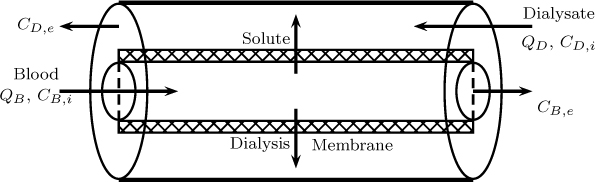
A mesoscopic model is illustrated here. Since the flow in the blood side is usually under laminar considerations, dispersion effects are added in the model. The dialysate side is modeled using plug flow. Model equations based on these flow pattern assumptions are shown next.
23.4.1 Model Formulation
The mass balance on the blood side follows the axial dispersion model and the following equation holds for the concentration of the solute in the blood stream. (Note that all concentrations are implied to be the cup-mixed average concentration and no special tag is shown in the notation.)
where is the transfer rate of the solute from the blood side to the dialysate side per unit perimeter and vB is the blood flow velocity. s is a shape parameter equal to zero for channel flow with R being half the width of the channel, while s is equal to one for a hollow fiber circular channel with R being the radius of the fiber.
The mass balance on the dialysate side is based on the plug flow and leads to
where QD and QB are the volumetric flow rate of the dialysate and blood, respectively. CD is the concentration of the solute in the dialysate side.
The transfer rate is modeled using resistances in series. The transfer involves three steps in series with each step offering its own resistance:
Transfer from the bulk of the blood stream to the inner surface of the membrane. This can be modeled using a mass transfer coefficient kL with 1/kL being the resistance.
Transfer across the membrane to the dialysate side. This can be modeled using a membrane permeance PM with 1/PM being the resistance.
Transfer from the walls of the membrane on the dialysate side to the bulk dialysate stream. This can be modeled using a mass transfer coefficient kD with 1/kD being the resistance.
The overall resistance is the sum of these three resistances:
Hence the transfer rate is given by
This completes the model formulation. The Danckwerts boundary conditions are used for the blood side since the dispersion model is used here while the inlet concentration of the solute is used at the inlet side of the dialysate. The model can be solved analytically after suitably combining Equations 23.13 and 23.14. Some details of how to proceed are indicated in exercise problem 23.13 and also in Ramachandran and Mashelkar (1980). The theoretical predictions for the parallel plate hemodialyzer were checked with the experimental data of Grimsrud and Babb (1966) and the data of Ramirez et al. (1971) and a close fit was observed. The sensitivity of model parameters were also investigated. In particular the diffusion coefficient of urea in blood is shear rate dependent (Hyman, 1975) due to the non-Newtonian nature of the blood. Hence sensitivity studies of model parameters are important in general. In this particular case, the sensitivity to variations in diffusivity of the solute was found to be less than 20%.
23.4.2 Model for Patient-Dialyzer System
The model was then coupled to simulate an artificial kidney system. A two-compartment model was used for the patient with part of the blood stream flowing through the dialyzer and recycled back to the patient. The schematic of this model is shown in Figure 23.8.

The mesoscopic model for the dialyzer shown earlier provides the clearance rate of the plasma compartment, which is equal to QB(CB,i – CB,e). The sensitivity to the exchange parameter was also demonstrated. Once calibrated, the model is useful to formulate a treatment protocol to control the concentration of urea in both the blood stream and in the tissue compartment.
One interesting factor was that the rate of removal has to be restricted so that significant differences in concentration in the two compartments do not develop. This can be achieved by decreasing the dialysate flow rate, increasing the solute concentration in the dialysate, or increasing the blood flow. Detailed results are not presented in the interest of brevity; please refer to Ramachandran and Mashelkar (1980) for the various parametric plots.
Summary
Models for many systems of biomedical importance can be built using the methodology shown in Part I of the book. Examples provided in this chapter should give you a good feel for development of such models and provide a useful collection of case study examples.
Oxygen transport in lungs is an important problem and also a good example of mass transfer modeling. The oxygen-hemoglobin equilibrium follows an S-shaped curve that is modeled by Hill’s equation. Oxygen binds cooperatively to multiple sites in hemoglobin; this is responsible for the S-shaped nature of the equilibrium curve.
The transport rate of oxygen in lungs can be calculated using a diffusion-reaction model to account for the reaction with hemoglobin. Transport through the capillary endothelium and convective mass transport in plasma are the two additional steps that are included in the model. These can be treated using an overall external mass transfer coefficient, which leads to a Biot number for external mass transfer. The internal transport and reaction in the red blood cells can be modeled using a Thiele modulus. This permits the calculation of an overall effectiveness factor. Hence the modeling approach is quite parallel to that for gas–solid catalytic reactions.
The local rate of oxygen transport can then be coupled to a mesoscopic model for the capillary to find the oxygen profiles as a function of the distance along the capillary and the distance needed to achieve a nearly complete saturation.
The transport rate of oxygen in tissue is another important problem and can be modeled by assuming the tissue is an annular cylinder covering the capillary. A zero-order reaction is normally assumed. We find that there is a critical Thiele modulus above which an oxygen starved region can develop at the outer radius of the tissue.
The local model for tissue consumption of oxygen can then be coupled with the mesoscopic model for the capillary to find the oxygen profile in the tissue and the length at which the oxygen concentration becomes nearly zero. For regions of low concentration of oxygen in the capillary, a lethal corner (an anoxic region) can develop at the outer radius of the annular cylinder representation of the tissue.
Distribution and metabolism of drugs in the body is the focus of pharmacokinetic analysis and compartmental models of various levels of detail are commonly used, the simplest being a one-compartment model. A two-compartment model consisting of a plasma and a tissue compartment is quite useful and simple. In further refinement, each compartment can be composed of three subcompartments and hence the models can be made fairly comprehensive and organ specific.
A dialysis unit is an example of a extracorporeal device and can be modeled as a countercurrent mass exchanger. Analytical solutions can be obtained for the exit concentration of the solute if a mesoscopic approach is taken and the clearance rate calculated from such a model can be incorporated in a two-compartment model for the patient to track the concentrations with time. The two-compartment model provides an estimate of the concentration in the tissue compartment, which is difficult to measure. Hence the model is useful to control both the tissue and the plasma concentration during the progress of the treatment.
Review Questions
23.1 What is Hill’s equation?
23.2 How does the carbon dioxide concentration in Hb affect oxygen dissociation?
23.3 What causes carbon monoxide poisoning?
23.4 What are the limiting transport steps in oxygen absorption in the lungs?
23.5 Explain how the effectiveness factor concept is useful to calculate the local rate of absorption of oxygen in lungs.
23.6 Define the characteristic distance for oxygen uptake and its meaning.
23.7 What is the physical picture upon which the Krogh cylinder model for oxygen transport in tissue is based?
23.8 When can an anoxic region develop in the tissue?
23.9 What is the lethal corner and what is the cause of it?
23.10 Justify the assumption that the blood (plasma) compartment is well mixed although it is in circulation inside blood vessels.
23.11 For pharmacokinetic modeling, when is a one-compartment model suitable and when it is not?
23.12 What is the PBPK model?
23.13 Show the similarity in the hemodialyzer modeling and modeling of a conventional chemical engineering separation process.
23.14 Discuss briefly how the patient-dialyzer linked model is useful in clinical applications.
Problems
23.1 Thermodynamic derivaton of Hill’s equation. Hill’s equation is based on oxygen binding to n sites simultaneously, which can be represented by the following reaction scheme:
L + nA ⇄ ALn
The notation A is used for oxygen and L is used for Hb (the ligand). Apply the law of mass action to this scheme and show that
[ALn] = K[A]n[L]
where the square bracket represents concentration. The total balance for the ligand requires n[ALn] + [L] = [LT] with LT being the total ligand concentration. Combine the two equations and shown that Hill’s equation results for oxygen saturation.
23.2 Total oxygen concentration in blood. Hematocrit refers to the volume fraction of RBCs in blood and is on the order of 0.45. Find the oxygen concentration in plasma using Henry’s law. Find the concentration of oxygen bound to RBCs using Hill’s equation. Find the total concentration of oxygen if the atmospheric pressure is 760 mm Hg at a sea level locations and 670 mm at a higher elevation of 1 mile.
The solubility coefficient of oxygen in plasma is equal to 1.125 × 10⁻¹¹ mole/cm3Pa. Note that the oxygen mole fraction in the lung is less than 0.21 since the lungs are saturated with water vapor at 37°C. Please correct for this as well.
23.3 Oxygen saturation in anemia patients. People with anemia have lower Hb concentration. Determine the level of oxygen saturation if the Hb level is 0.1 g/mol compared to the normal level of 0.14.
23.4 Overall effectiveness factor for oxygen uptake. Calculate the effectiveness factor for the oxygen uptake in RBCs based on the following parametric values suggested by Truskey et al. (2004):
– Permeability of the capillary walls = 0.387 cm/s
– Mass transfer coefficient in plasma = = 0.44 cm/s
– Effective length of RBC = 1.35 μm
– Diffusion coefficient of oxygen in RBC = 6.0 × 10⁻⁶ cm2/s
– Rate constant for first-order reaction ≈ 1000 s–1.
23.5 Length needed for saturation. Calculate the characteristic parameter and the length needed for a capillary to be saturated with oxygen for the following conditions: blood flow velocity = 2.5 mm/sec; hematocrit value = 0.45. For other parameters use the values from the previous problem.
23.6 Application of Krogh model. Apply the Krogh model to the following data (from Truskey et al., 2004) to find the maximum intercapillary radius for no anoxic region formation. Metabolic rate = 1 × 10⁻⁷ mol/cm3s, a zero-order reaction; capillary radius = 1.5 to 4 μm; DO2 = 2 × 10⁻⁵ cm2/s in tissue; oxygen concentration in blood at the given point: 4.05 × 10⁻⁸ mol/cm3.
23.7 Oxygen variation with length in a capillary near tissue. Solve Equation 23.11 for CA versus z for the data in the previous example. The velocity of blood is 2 mm/s. The inlet concentration of oxygen is 19.88 ×10⁻³ M. Consider two cases. First, assume no anoxic region develops in the tissue. Find the length at which the oxygen concentration becomes zero. Second, assume an anoxic region forms and find the length at which the lethal corner can develop.
23.8 Model for NO distribution in blood and tissues. NO is a vasodilator and is produced in the endothelium of the blood vessel and the tissue epithelelium. NO then diffuses into the capillary as well as into the tissues, and also undergoes a reaction. A schematic of the process is illustrated in Figure 23.9.

Figure 23.9 Schematic of a model for NO generation and diffusion+reaction in both tissue and the capillary.
The concentration profile of NO is important to assess the distance over which NO acts in the tissue. The NO concentration should remain above a critical value for it to be effective. The Krogh cylinder model is useful here. Assume the reaction is first order in NO. Show that the following equation is then applicable:
Show that this applies both to the capillary (0 to RC) and the tissue (RC to R0). However, the equation needs to be solved separately for the two regions since the reaction rate is not the same in the two regions. The boundary condition at r = RC also has to be matched for the two regions to get the complete solution. The boundary conditions at r = 0, the center of the capillary, and r = R0 the outer edge of the tissue, are the no flux conditions. At r = RC the concentration is continuous. Note that the thickness of the endothelium is ignored. The generation in the endothelium provides the second matching condition at r = RC. Show that the following condition holds at r = RC:
Simulate and plot the NO profile in the blood and capillary for the following set of parametric values taken from Truskey et al. (2004):
– Production rate = 5.5 × 10⁻¹² mol/cm2s
– Rate constant for reaction in blood = 1000 s–1
– Rate constant for reaction in tissue = 0.01 s–1
– Diffusion coefficient in blood = 4.5 × 10⁻⁵ cm2/s
– Diffusion coefficient in tissue = 3.3 × 10⁻⁵ cm2/s
– Radius of the capillary - 25 μm
– Outer radius of the tissues = 100 μm
23.9 Nutrient limitation in tumor growth. Tumors pull nutrients needed for their growth from the surrounding tissues. If the tumor size becomes large, a region can develop inside the tissue where the nutrient concentration drops below a critical value. The growth is then limited by lack of nutrients. An illustrative concentration profile is shown in Figure 23.10.

Figure 23.10 Concentration profile for nutrient diffusion with a zero-order reaction in a tumor showing the no growth region within the tumor.
Solve the model for a zero-order reaction in spherical coordinates. Develop an expression for the radius of the tumor at which the center concentration drops below a critical value. Note that the size of the tumor will be limited by this value because nutrient starvation occurs above this value. The model applies to the avascular stage of growth, that is, when the tumor has not developed its own blood vessels.
23.10 Tumor growth: inhibitor limited model. Tissues generate inhibitors, which are needed to control growth and other processes. Tumors also do this. Develop a diffusion-reaction model for a spherical shaped tumor that generates an inhibitor by a zero-order reaction and also destroys it by a first-order reaction. Solve for the concentration profile. An illustrative profile of the type shown in Figure 23.11 will be obtained.
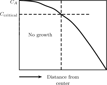
Figure 23.11 Concentration profile for inhibitor-limited growth in a tumor. Tumor growth is confined to the outer shell.
The boundary condition at the edge of the tumor can be a Robin or Dirichlet type condition. The Dirichlet condition with zero concentration applies if the permeability of the tumor membrane is rather large. Set up and solve the model for both cases. The tumor growth will stop in regions where the concentration of the inhibitor is above a critical concentration (see Figure 23.11). Solve and plot the profiles for concentration for various radii and mark regions where the tumor ceases to grow, assuming a value for the critical concentration.
23.11 Solution for a three-compartment model. The plasma concentration of small molecules is best fitted by a three-compartment model. Truskey et al. (2004) suggests a central compartment where a drug is injected and cleared and two peripheral compartments as shown in Figure 23.12.

Figure 23.12 A three-compartment model. The drug is injected and cleared from the central compartment (1), which exchanges mass with two peripheral compartments (2 and 3).
Set up the model and solve for the central compartment concentration as a function of time using the matrix method. Show that the concentration in the plasma (central compartment) can be represented as a triexponential solution of the following form:
Cp = Cp0 [ 1 exp(– λ1t) + α2 exp(– λ2t) + (1 – α1 – α2) exp(– λ3t)]
Explain the relation of the constants α s and λ s to the volume parameters, clearance rate, and exchange rates.
23.12 Analytical solution to the dialyzer model. Equations 23.13 and 23.14 can be combined and the transfer rate term can be eliminated. The resulting equation can be integrated to get a relation between the dialysate concentration and the blood concentration. Show that the following equation results if this procedure is applied:
Now use this in Equation 23.13 to get a differential equation for CB. This equation is very similar to the axial dispersion model; the only difference is that the coefficients are modified to include QB/QD ratio terms. The solution has the same form as the axial dispersion model and provides an analytical solution to the dialyzer model. Set up this equation and solve for the exit concentration of the solute in the blood stream.