
Chapter 24. Electrochemical Reaction Engineering
Learning Objectives
After completing this chapter, you will be able to:
Understand basic definitions used in electrochemical engineering and their relation to equivalent concepts in chemical reaction engineering.
Evaluate the minimum voltage requirements from thermodynamic considerations of the reactions taking place at electrodes.
Review two common kinetic models for electrochemical reactions: the Butler-Volmer model and the Tafel model.
Show how mass transfer affects the rate and understand the notion of the limiting current.
Set up a model and design a simple electrochemical process, copper electrowinning from a leach solution.
Show how the current versus voltage relation in a fuel cell is related to mass transfer and the reaction taking place in the system.
Show the various transport steps in a Li-ion battery and their importance in modeling these systems.
This chapter deals with electrochemical reaction engineering, an often neglected topic in undergraduate chemical engineering and textbooks. This is a classical as well as emerging area and has important applications in energy engineering and chemical industries. Sodium hydroxide was probably the first chemical to be made on a large industrial scale by electrolysis of sodium chloride solution and hence electrochemical engineering can be considered to be older than chemical engineering. The interest in electrochemical routes to make chemicals on an industrial scale continues and electro-organic synthesis is emerging as a growth area, especially in the pharmaceutical industry. In the modern context of energy production and storage, electrochemical engineering has become a major design tool. Hence it is important for chemical engineers to understand the basic concepts of these systems and to learn how one goes about the analysis of them. Specialized books are available but a primer such as given in this chapter is very useful to get started and to develop basic knowledge of modeling of electrochemical reactors.
The chapter is organized in the following manner. First we show the basic definitions needed to understand the system. Then the thermodynamics of electrode reactions and the use of oxidation and reduction potentials is discussed, followed by models for kinetics of electrode processes. We then integrate the kinetics and transport effects illustrated in Chapter 16 (Section 16.5 in particular) and show how they can be coupled with basic conservation laws to develop models for electrochemical systems. Simple applications of the kinetics and mass transfer are then presented for three industrially important systems. Overall the study of this chapter will provide a basic understanding of electrochemical reaction engineering and you will be in a position to understand specialized textbooks and papers in this area.
24.1 Basic Definitions
Electrochemical reaction engineering introduces several new concepts and terminologies not so familiar to chemical engineers and there is a need to define these and demonstrate how they relate to classical reaction engineering terms. This permits the translation of the vocabulary used by electrochemical engineers to chemical engineers.
A typical electrochemical reactor or cell consists of an electrolyte with two electrodes on either side forming an electrochemical cell: an anode and a cathode where an oxidation and a reduction reaction takes place, respectively. The electrons generated or consumed in these reactions flow through an external circuit. The ions move within the electrochemical cell across the electrodes. Hence a current flows through the system. The current flow is taken in the opposite direction to the electron flow. A voltage is applied to maintain the current flow in an electrolyzer. A voltage will be generated if the reaction is spontaneous in which case the system acts as a fuel cell.
24.1.1 Anodic and Cathodic Reactions
Reactions are generally represented as oxidation and reduction. Oxidation is the release of electrons. Electrons are the product and appear on the right-hand side of the reaction scheme. This reaction is also referred to as an anodic reaction. The electrode where an oxidation reaction is taking place is called the anode.
Reduction is the reaction where a electrons are the reactant. The electrode where a reduction reaction is taking place is called the cathode.
A schematic diagram illustrative of the processes taking place at the electrode is shown in Figure 24.1. Here a single-step electron transfer process is shown but often multiple electron transfers will be involved in many practical situations. R is the species undergoing oxidation to produce O.

Figure 24.1 Illustration of a simple electrode reaction taking place at an anode and a cathode. A single electron transfer reaction is shown.
24.1.2 Half Reactions and Overall Reaction
Two halves make a whole. In electrochemical reactors two half reactions (anodic and cathodic) have to occur so that a current flow can occur in the external circuit across the cell. These reactions should add up to an overall reaction.
One of the half reactions may even be a parasitic reaction leading to no useful products, but is a necessary part of the overall process. In some cases both reactions can lead to useful products; such reactions are known as paired synthesis. Here both the anodic and cathodic processes lead to useful products. Industrial applications of paired synthesis are not so common; this is often called the electrochemist’s dream. In inorganic chemical industry, chloralkali is example where both the anodic and cathodic products lead to useful products. An illustrative sketch of this process is shown in Figure 24.2. The two half reactions are also shown and the overall reaction is the sum of the two:

Figure 24.2 An illustrative electrochemical reaction: NaCl electrolysis. Note that a diaphragm or membrane is used to separate the anodic and cathodic regions.
This is the sum of the two half reactions shown in Figure 24.2. The overall reaction has a positive change in free energy and is therefore not spontaneous. Hence a voltage has to be applied in order to drive the reaction from the left to right. How much voltage is needed depends on the rate of reaction (or equivalently the current in the system) and is addressed by a voltage balance shown later.
A second example of half reactions and the overall reaction is the fuel cell shown in Figure 24.3. Here hydrogen enters the anode side and air or oxygen flows on the cathode side and the overall reaction is
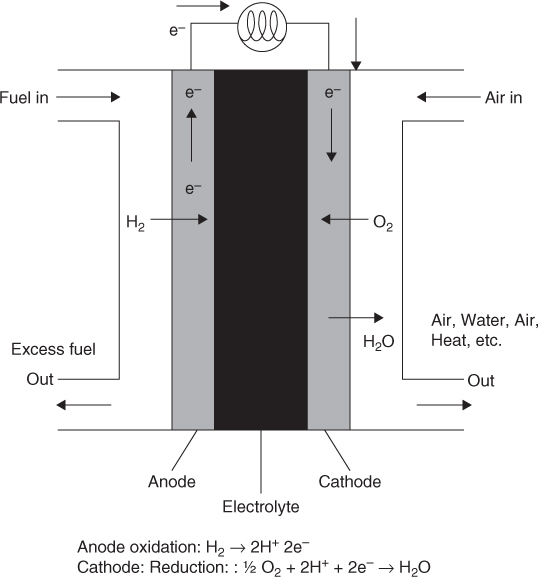
This is split into two half reactions, which are shown in Figure 24.3. The electrons flow from the anode to the cathode in the external circuit. Positive ions (H+) are generated at the anode due to the oxidation of the H2 gas and are transported from from anode to cathode across a proton exchange membrane (PEM). This membrane separates the anode and the cathode and allows passage of only hydrogen ions to the cathode. The hydrogen ion then participates in the reaction with oxygen at the cathode to form water.
The free energy change associated with the overall reaction in a hydrogen fuel cell is negative and hence the reaction is spontaneous. It therefore generates a voltage. The value of the voltage depends on how much current is being drawn from the system and is addressed later.
24.1.3 Classification of Electrode Reactions
Depending on the nature of the product formed in the electrode reaction, the process can be broadly classified into four types, which are shown schematically in Figure 24.4. These are shown for a process taking place at a cathode, that is, where a reduction is taking place. A similar type of classification applies to an anodic process as well. The reduced product in a cathodic reaction can belong to four categories, as shown in Figure 24.4.

Figure 24.4 Classification of electrode reaction depending of the nature of the product formed by electrochemical reaction.
The simplest case is where both the reactant and product stay in the liquid phase. A common example is the ferrous from ferri reduction. This is often used as a test reaction to measure mass transfer coefficients from the bulk solution to the electrode.
The second case is where the product is solid that deposits on the electrode; this has important applications in metal refining industries.
The third example is where the product is a gas. The gas evolution has important consequences as it leads to a two-phase mixture in the system, leading to reduced electrical conductivity and other associated design issues. It can also provide the benefit of increased mass transfer rate at the electrode due to convective mixing caused by the gas bubbles.
Finally the last case is where the electrode supplies enough energy to provide a radical, which reacts further with a liquid reactant (near the electrode) to form the useful product. Such examples are found in electro-organic synthesis.
Each case needs some adjustments and modifications in the engineering of the process and the associated reactor design. Further details are not addressed here.
24.1.4 Primary Variables
Two primary variables are needed in order to analyze an electrochemical process: the current and the potential or the applied voltage, as already discussed earlier. These are reiterated in the following.
Current: This is a measure of the rate of flow of electrons in the external circuit and the flow of ions within the electrolyte. The units are Coloumb/sec, abbreviated as ampere, A. The current density is the flow per unit area of the electrode; the units are A/m2. It is important to note that the current is a measure of the overall reaction rate at the electrode surface. The following relation holds for a single reaction:
where NAs is the rate of surface reaction (electrode reaction) per unit area, i is the current density, and n is the number of electrons transferred in the electrode reaction. F , the Faraday constant, is the conversion factor from number of electrons to moles. It represents the amount of electric charge carried by one mole of electrons; the value is 9.65 × 10⁴ C/mol of electrons.
Voltage: This is a measure of the potential energy associated with a unit charge. If a positive charge of 1 C has been moved by one unit of length of 1 m it acquires a potential energy of 1 V. Hence 1 V is equal to 1 J/C. An electrochemical reaction with an almost zero current needs (or produces if it is a fuel cell) a minimum (maximum) voltage, which is dictated by thermodynamic considerations. The calculation of this minimum voltage is addressed in the following section.
Calculation of the current versus voltage relation require consideration of transport effects and kinetic models for the electrode reactions. This is addressed in Section 24.5.
24.2 Thermodynamic Considerations: Nernst Equation
Consider an electrode in contact with a solution with the following reaction taking place on the electrode surface:
R → On+ + ne–
The chemical potential difference drives the reaction.
Note that at least one of the species R or O has to be a charged species or both of them can be charged species to balance the negative charge due to electrons. The point to note is that the net charge on the left-hand side must balance the net charge on the right-hand side. An example, where O is a charged species and R is not, is
Ag → Ag+ + e–
An example where both are charged is
F e++ → F e+++ + e−
which is the ferri–ferrous reaction often used as a test model reaction in electrochemistry.
The equilibrium potential (denoted as Eeq) is defined as the potential difference between the electrode ϕm and the solution ϕs under conditions of no reaction or equivalently no net current. It should be noted that the ϕ’s do not have an absolute value and are determined in accordance with a reference electrode whose potential, is assigned a zero value. It is similar to the gravitational potential, which uses a reference elevation whose potential is set to zero. Eeq, being a difference of two potentials, has an absolute value. An equation for this will now be derived.
The forward reaction and the backward reaction take place at the same rate under the condition of equilibrium. Hence the sum of the chemical potential of all species on the left-hand side must balance the sum of the chemical potential of the species on the right-hand side. An equation for Eeq can be derived based on this concept, which is the famous Nernst equation in electrochemistry.
The net driving force in the forward direction, that is, toward the oxidation reaction or the anodic reaction, is taken as the difference in the chemical potential between the reactants and the products:
Driving force = μR – (μO + nμe)
where μe is the chemical potential of the electrons at the metal surface. The chemical potential in turn is related to the concentration of the species. Thus for species R the chemical potential is represented as
where Rg is the gas constant, μ0R is the chemical potential in the standard state, and CR is the concentration expressed as mol/L. This presumes that the standard state is taken as 1 M solution. We assume that R is not charged but the final result will be same if R is also charged (due to the sotchiometric balance of charges on both sides of the equation).
Similarity for species O the chemical potential is
where ϕs is the electric potential of the solution adjacent to the electrode. Here we have included the electrochemical potential for species O since this is a charged positive species.
The chemical potential of the electrons depends on the potential of the metal or the electrode that is in contact with the solution and can be varied by adjusting the potential of the metal or the electrode ϕm. Then the chemical potential of the electrons is equal to
Note that both ϕs and ϕm are relative as mentioned earlier as well. We assume here that these are measured with reference to a standard electrode that has a stable and reproducible potential. Of course the final result is not affected since it is the difference between the metal and the solution potential that will matter.
Net driving force (d.f.) is therefore equal to
For no reaction to take place the driving force has to be zero. This represents the condition for equilibrium. The corresponding potential of the metal with respect to the adjacent electrolyte solution is referred to as Eeq:
Eeq = ϕm – ϕs
Setting the net d.f. as zero in Equation 24.2, we get
We define E0 as
This is the free energy change (expressed in electrical potential units) when all the species are at their standard state.
Equation 24.3 is written in terms of E0 as
This is the Nernst equation. If all species are in their standard state then Eeq = E0.
The above represents the equilibrium state of the system. No current flows in such cases. Any reaction needs a departure from equilibrium conditions; this is accomplished by applying a potential at the electrode different from the equilibrium value.
Note that there is no unique value to E0. Hence this is referred to some comparative values. The hydrogen (H2) to hydrogen ion H+ reaction is given a value of zero. Then a value can be assigned to other electron transfer reactions. These values, known as oxidation potential, are tabulated in many books. Some typical values are given in Table 24.1.
Table 24.1 Oxidation Potential for Some Standard Half Reactions. Reactions at the Top are Thermodynamically Favorable while for those Near the Bottom the Reaction is Favorable in the Reverse Direction
Reaction |
Standard Potential |
Na → Na+ + e– |
–2.714 |
Al → Al+3 + 3e– |
–1.66 |
1/2H2 + OH– → H2O + e– |
–0.828 |
Zn → Zn+2 + 2e– |
–0.763 |
H2 → 2H+ + 2e– |
–0. |
Ag → Ag+ + e– |
0.7991 |
Cu → Cu+2 + 2e– |
0.337 |
2H2O → O2 + 4H+ + 4e– |
1.229 |
2Cl– → Cl2 + 2e– |
1.3595 |
Note that some books tabulate the reduction potential, that is for the reverse reactions shown in Table 24.1. These values will then be the negative of the values in the table. Hence caution has to be exercised in using these values.
Note that in the table E0 has the same sign as ΔG (the free energy change under standard conditions). Hence reactions with negative values are favorable to the right (anodic) while those with positive values are cathodic and tend to occur to the left. For example, sodium prefers to stay as Na+ since the standard potential is minus 2.714. Similarly chlorine prefers to be Cl– since the potential is plus 1.3595. The ionic bond keeps them together and thus we find only NaCl in nature.
24.2.1 Equilibrium Cell Potential
In an electrochemical reactor two half reactions, one at an anode and one at a cathode takes place. The net potential difference at equilibrium is found from the difference:
If ER,eq is negative, then the reaction is spontaneous. The system can be used as a fuel cell to generate energy. In this case, the magnitude of ER,eq will be the maximum voltage that can be generated in a (single stack) fuel cell for the given reaction. This will apply to a zero current situation.
Example 24.1 shows the application of thermodynamic calculations in electrochemistry.
Example 24.1 Minimum Voltage Calculations
Using the oxidation potential in Table 24.1 find the minimum potential to decompose NaCl in a diaphragm cell. Assume the concentration is 1 M, that is, use standard state values. Repeat for a hydrogen + oxygen reaction in a fuel cell.
Solution
The overall reaction is
We need to write this as two half reactions, which are shown in Figure 24.2. From the table we find that the anodic reaction of Cl– going to Cl2 has a potential of 1.3595 V. The cathodic reaction of water going to hydrogen and OH– has a potential of 0.828 V. Note that the value shown in Table 24.1 is if the reaction is anodic but the reaction is cathodic and hence in the reverse direction. We therefore changed the sign on the potential.
The minimum voltage is the sum of anodic and the cathodic potentials and hence
E0 = 1.3595 + 0.828 = 2.1865V
This is the minimum potential needed to drive the reaction. Additional voltage needs to be applied to drive the reaction; this will depend on the kinetics of the reaction (as well as the mass transfer steps), which is discussed later. If the NaCl concentration is not 1 M, then a concentration correction is applied using the Nernst equation, Equation 24.4.
For the hydrogen fuel cell the overall reaction is
This needs to be written as two half reactions, one corresponding to the anode reaction or the oxidation and the second corresponding to the cathode reaction, which is reduction.
At the anode hydrogen gas is oxidized to H+ions; this has a potential of zero, if hydrogen is at the standard condition of 1 atm pressure.
At the cathode the reduction of oxygen is the reaction taking place: 1 2
The potential for this is E cathode = –1.229 V (reverse of the value in Table 24.1 since it is now from right to left). This potential applies if the oxygen partial pressure is 1 atm. Hence E0 = 0 – 1.229V under standard conditions. As this is negative, the reaction is spontaneous and generates energy.
If air is used, the oxygen partial pressure is 0.21 atm. Now using the Nernst equation (Equation 24.4) (RgT/nF)ln(0.21) is added, giving E0 = –1.119 V.
The effect of temperature on the cell potential is indicated here. The equilibrium potential calculated at the standard condition of Tref = 298 K is corrected for other temperatures as follows using a linear relation:
From thermodynamics, we have
Here ΔS0 is the standard entropy change for the overall reaction.
24.3 Kinetic Model for Electrochemical Reactions
Now depending on the actual applied potential of the electrode (metal) the reaction can be driven either to the right or to the left. Let us define the difference between the actual applied potential and the equilibrium potential as η, the surface overpotential:
η = E – Eeq
If η is greater than zero, the driving force term is positive and hence oxidation is favored. If η is less than zero, the driving force term is negative and hence the reverse reaction (reduction) is favored. A kinetic model should reflect these effects of the applied potential. The model should also be thermodynamically consistent.
The effect of electrode potential is shown schematically in Figure 24.5. The forward reaction (oxidation) is an electron removal process from the solution; the rate increases as the electrode potential becomes more positive, since the electrons are attracted to the positively charged electrode. The reverse (reduction) happens when the electrode potential is reduced; the electrons prefer to leave the electrode as shown in Figure 24.5.

Figure 24.5 Effect of electrode potential on the direction of electron transfer. The left side represents the metal or the electrode while the right side represents the solution adjacent to it.
The process can also be interpreted using the Fermi level of the electrons in the electrode; this is illustrated in Figure 24.6. The Fermi level is a measure of the chemical potential of the electrons. At equilibrium conditions the Fermi levels of the electrons in the electrode and in the HOMO (higher occupied molecular orbital) of the solution are the same as shown by the dashed line in Figure 24.6. An increase in electrode potential causes the Fermi level of electrons in the electrode to decrease, causing a jump of electrons from the solution to the electrode. Oxidation takes place. The opposite happens when the electrode potential is reduced.

Figure 24.6 Fermi level interpretation of the effect of applied electrode potential on the direction of electron transfer.
24.3.1 Butler-Volmer Equation
The rate for oxidation reaction, rf or ra (where a stands for anodic), is assumed to be exponentially proportional to βE where β is a factor between 0 and 1 called the symmetry factor:
rf = ra = kf CR exp(nf βE)
where f is used as an abbreviation for F/RgT and has a value of 44.2 V at 298 K. This is similar to E/RgT in the Arrhenius equation. n is the number of electrons transferred.
The rate of reverse reaction should decrease with an increase in E. Hence
rb = rc = kbCO exp(–nf(1 – β)E)
The net rate is therefore
Rate = kf CR exp(nf βE) – kbCO exp(–nf(1 – β)E)
At equilibrium we have
0 = kf CR exp(nf βEeq) – kbCO exp(–nf(1 – β)Eeq)
Hence
Also, the ratio CR/CO is given by Nernst equation as we are looking at equilibrium conditions. Hence rearranging the Nernst equation we have
Substituting this into Equation 24.7, we find that the backward constant is related to the forward constant as
The rate constants kf and kb are not independent but are related to each other. This is because the rate should be zero at equilibrium. For ordinary chemical reactions kf /kb = Keq and the above relation is the electrochemical equivalent to this classical relation.
Hence the rate is
Rate = kf CR exp(nf βE) – kf exp(nfE0)CO exp[–nf(1 – β)E]
It is customary to define a standard rate constant k0 defined as follows:
k0 = kf exp(–nf βE0)
or
kf = k0 exp(nf βE0)
Note: k0 has the same units as the heterogeneous rate constant for a first-order catalytic reaction, m/s.
Hence the rate can be expressed as
r = k0[CR exp[nf β(E – E0)] – CO exp[–nf(1 – λ)(E – E0)]]
Multiplying both sides by nF we get the following equation for the current density i, which is equal to nFr:
This is the Butler-Volmer kinetic model for an electrode reaction in the classical form. This model is also thermodynamically consistent. At equilibrium the rate or correspondingly the current density i can be shown to be zero.
Overpotential Form
Let R* and O* be two reference concentrations. These could, for example, be the bulk concentrations or the inlet concentration to the electrolyzer. Let Eeq be the corresponding equilibrium potential, which can be calculated for the Nernst equation. Then let
which is also equal to
since the rate in the forward direction is the same as the backward direction under equilibrium conditions.
The parameter i0 is known as the exchange current. Equilibrium is viewed as a dynamic process here with equal current flowing back and forth between the solution and the electrode; the exchange current is a measure of this process. Clearly the exchange current may be thought of as the intrinsic electro-catalytic activity of the electrode. It is a measure of the charge transfer process between the electrode and a solution at a given reference concentration. Therefore it can be linked to, for example, the work function of the metal. Note that io is often reported using the standard conditions as the reference concentration, but this is not always stated clearly.
The equation for the current i given by Equation 24.9 can then be represented as
Let η be the overpotential defined as E – Eeq. Then
which is the overpotential form of the Butler-Volmer equations.
If CR and CO (concentrations in the solution adjacent to the electrode) are themselves chosen as the reference concentrations then this reduces to
i = i0 [exp(nf βη) – exp(–nf(1 – β)η)]
This form of the Butler-Volmer equation is applicable, for example, when there is no mass transfer resistance, that is, the bulk and the surface concentrations are the same.
If β = 1/2 the Butler-Volmer equation can be written in hyperbolic form:
Usually the magnitude of η is high so that the reaction is driven to only one side. The reverse reaction can then be dropped, leading to yet another form of the equation:
Some typical values for i0 are shown in Table 24.2:
Table 24.2 Typical Range of Values for the Exchange Current
Process |
Conditions |
i0 A/m2 |
H2 evolution on Pt |
0.5 M H2SO4 |
10 |
H2 evolution on Ag |
7 M HCl |
0.012 |
Cu deposition |
1M CuSO4 |
0.2 |
Temperature Effect
The values of i0 measured at temperature Tref are corrected to any other temperature T by Arrhenius’s law:
Here Ea is the activation energy for the electrode reaction.
24.3.2 Tafel Equation
The Tafel equation is a simplified form of Equation 24.11 and is obtained by taking the logarithm on both sides. This is usually written as
η = a + b log(i)
where a and b are the kinetic parameters of the Tafel model.
24.4 Mass Transfer Effects
If there is a mass transfer resistance near the electrode then the surface concentration and the bulk concentrations will be different. The mass transfer effects are usually accounted for by the film model. Consider the reduction reaction scheme O going to R. An example would be copper ions going to a cathode and reacting there to deposit Cu. The rate at which species O is transported from the bulk (which we assume to be at a concentration of CO,b) to the electrode is
NA = kLfd(CO,b – CO,s)
Here CO,s is the surface concentration. fd is the enhancement in mass transfer due to electric field. kL is the mass transfer coefficient in the absence of electric field.
The preceding equation for the rate of mass transfer can be expressed in terms of current (multiply by nF ):
Let us define iL, termed the limiting current, as
iL = nF kLfdCO,b
Then the rate of mass transfer (expressed as a current) is
The electrochemical reaction occurs in proportionality to the surface concentration and exponentially to the electrode overpotential. The current can be written using the Butler-Volmer equation:
The reverse current (1 – η) term is assumed to be small and neglected here. Also, the absolute value for η is used since we are looking at a reduction here. Note that η is negative for a reduction reaction.
At steady state the two currents are equal:
im = iR = i
Hence Equations 24.14 and 24.15 can be set equal to each other and CO,s/CO,b can be eliminated. Then either of Equation 24.14 or 24.15 can be used to find i. The final expression can be found easily as
which is a version of the law of addition of resistances.
Two limiting cases can be identified:
Mass transfer control: iL << i0 exp(nf β|η|)
The current is equal to iL.
Electrode reaction control: iL >> i0 exp(zf β|η|)
The current is now given by Equation 24.15 with CO,s set the same as CO,b.
The analysis is similar to the heterogeneous reaction discussed in Section 6.4.1.
At low overpotential the process is likely to be electrode controlled. As the overpotential increases the rate of electrode reaction increases and mass transfer resistance starts to become important. Beyond this point further increase in overpotential will not cause any further increase in rate.
24.4.1 Concentration Overpotential
Note that concentration drop due to mass transfer creates a potential gradient between the electrode and the bulk solution. This is known as the concentration overpotential or the concentration polarization. The expression for this was presented in Section 16.5, which should be revisited now. The expression was presented for a simple binary electrolyte MX with M reacting at the cathode. The anion X did not participate in any reaction at the cathode and hence its combined flux was set to zero. The migration part of the combined flux of X set up an electric potential in order to cancel out the diffusional part. The expression is repeated here:
Role of Supporting Electrolyte
The expression is valid only if there is a single electrolyte, MX here. If there is a supporting electrolyte NX the expression for the potential difference has to be calculated using the Nernst-Planck equation for each of the ions, M+, N+, and X–, and the electroneutrality conditions. Exercise problem 14 in Chapter 16 addressed this. In general the concentration overpotential gets smaller in the presence of a supporting electolyte.
24.5 Voltage Balance
The voltage balance shows how the applied voltage is distributed among the various transport steps and reaction steps. It is an important component in the analysis of electrochemical reactions. It is similar to energy balance in classical chemical reactions.
The minimum voltage needed to carry out an electrochemical reaction is given from thermodynamic considerations and is equal to ER,eq, given by Equation 24.5. The actual voltage to be supplied depends on the current carried in the external circuit.
To generate an anodic current we need an overpotential ηa, which can be calculated from the Butler-Volmer equation. This is the additional voltage needed to produce a current. The current at the cathode is the same as that in the anode. Additional overpotential is needed for this current, which is the magnitude of the cathodic overpotential. In addition there is a solution voltage drop due to the migration of ions in the bulk liquid from one electrode to other. Additional voltage drop occurs if there is membrane or diaphragm separating the anodic and cathodic regions. Hence the total voltage that needs to be provided to maintain a certain value of the current is
Here ϕa(C) is any additional potential drop caused by mass transfer effects in the film near the anode. ϕc(C) is a similar term for the potential drop in the cathodic diffusion layer. An illustrative diagram is shown in Figure 24.7.
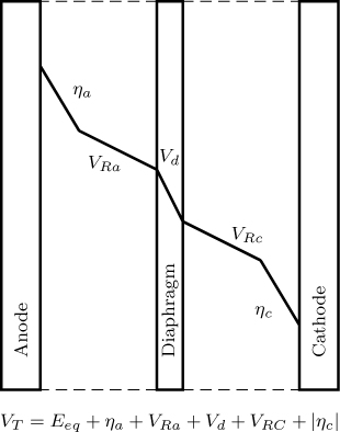
Figure 24.7 Voltage distribution in an electrochemical reactor. The concentration overpotential is not shown and should be added if there are significant mass transfer effects.
As an example, the potential needed for the various steps in NaCl electrolysis is presented in Table 24.3 at a current density of 2000 A/m2. We find the cathode reaction consumes more energy than the anodic reaction. The membrane also adds to a significant voltage drop. The total voltage to be applied is on the order of 3.65 V. A more detailed calculation of voltage balance is undertaken in the next section by taking a specific case of copper electrowinning.
Table 24.3 Illustration of Various Voltage Drops for NaCl Electrolysis
Equilibrium |
2.17 |
Anodic overpotential |
0.03 |
Diaphragm drop |
0.60 |
Solution drop |
0.35 |
Cathodic overpotential |
0.30 |
Metal hardware |
0.20 |
TOTAL |
3.65 V |
If the reaction is spontaneous, then ER(eq) will be negative. The system can be used as a fuel cell in that case. Let V0 be the magnitude of this, which is a positive quantity. Then V0 is the maximum voltage the fuel cell can generate and this will be at zero current. Any current needs an overpotential and can cause a voltage drop. Hence the voltage balance in a fuel cell is written as
An example of this calculation is shown in Section 24.7.
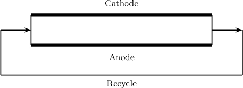
24.6 Copper Electrowinning
The various concepts are put together and applied in this section. A specific application to copper eletrowinning is considered here but the methodology is general and is applicable to a wide variety of electrosynthesis processes.
The overall reaction in Cu processing from leach solutions of Cu salts can be represented as
Cu++(aq) + H20(aq) → Cu(m) + 2H+(aq) + 1/2O2(g)
This is split into two half reactions. The anodic reaction is
H20(aq) → 2H+(aq) + 1/2O2(g) + 2e– E0 = 1.229V
This is the oxygen evolution reaction while the cathodic reaction is the desired reaction of copper deposition:
Cu++(s) + 2e– → Cu(s) E0 = –0.337V
The thermodynamic cell potential is calculated as the sum of these potentials.
24.6.1 Operating Current Density
The diffusion limiting current (DLC) calculation is an useful start; this is calculated from mass transfer considerations. It sets the maximum production rate that can be achieved. The corresponding voltage can also be calculated and operating above this value will not produce any further increase in the rate of reaction. From the discussion in Chapter 16 we note that
The factor 2 (the migration factor) is replaced by 1 in the presence of a supporting electrolyte (usually H2SO4). n is the number of electrons transferred, which has a value of two here. DM /δf is replaced by the mass transfer coefficient, km, and the limiting current can be calculated as
A value for the mass transfer coefficient is needed for further calculations and a number of correlations are available for this purpose. A limiting Sherwood number of 7.54 can be used as a simple approximation for flow between two parallel plates. For a more detailed correlation see Section 9.5.3, which is applicable if the flow is laminar. Hence km = 7.54D/2h. Using D = 2 × 10⁻⁹ m2/s and a gap width of 5 mm we find km = 1.5 × 10⁻⁶ m/s. Bulk copper concentration is taken as 600 mol/m3 in this example. Using these values in the equation for the limiting current we find iL = 174 A/m2.
The actual value of DLC is expected to be higher since fully developed mass transfer may not have developed; hence the above value is an underestimate. A number of similar correlations have been proposed and these may be used as appropriate. The effect of gas evolution is to increase the rate of mass transfer as well; this has not been reflected in our calculations. The value calculated is, however, close to that reported by Beukes and Badenhorst (2009).
In operating reactors a current lower than the DLC is used so as to achieve a good adherent product. We take a value of 0.8 times the DLC for further calculations and calculate the voltage needed to achieve this current. Hence the current i is as 140 A/m2.
24.6.2 Voltage Balance
The thermodynamic potential shown earlier is for standard conditions (1 M solution). This is corrected for concentration dependency using the Nernst equation and the value is obtained as 0.892 V since the concentration is 0.6 M in this case study.
Anodic overpotential is calculated using the Tafel equation for a lead anode. The Tafel constants are taken from Beukes and Badenhorst (2009):
ηa = 0.303 + 0.12 log10(i)
This is calculated as 0.5604 V. The cathodic overpotential is calculated using the Butler-Volmer equation:
where we ignore the anodic part of the reaction (the reverse reaction term) and take the β factor as one. A first-order dependency is used here. i0 is the exchange current and is a function of the copper concentration:
In SI units the value of the exchange current, i0, is 245 A/m2 using k = 1 Am–2(m3/mol)–.5 as reported by Lapique and Storck (1985).
The surface concentration can be eliminated using the limiting current:
Using this in the Butler-Volmer equation and taking the logarithm on both sides, the following equation can be obtained for the cathodic overpotential:
This is a combined equation and includes the overpotential due to the cathodic reaction and due to the concentration drop in the Nernst diffusion layer (film) near the cathode. The value is calculated as 0.335 V.
The ohmic potential is calculated as
where κ is the specific conductivity and is calculated as
For the given system κ = 78.47 S/m. Hence the ohmic drop for the given current is only 0.05 V. The supporting electrolyte minimizes the voltage drop across the solution. The total potential is then found as 2.18 V and is in the range of values used commercially.
24.6.3 Meso-Model for the Electrolyzer
All the factors of importance have been put together and the local rate of reaction (in terms of i for electrochemical engineers) can be related to the required voltage for a given copper concentration.
This can be put into a mesoscopic model to track the variation of copper concentration as a function of length in a parallel plate electrolyzer.
The model is set up as
where i/nF is the local rate of reaction. Here W is the cell width and x is the coordinate along the cell length. One slight problem is that i is not known at each position and what is known usually is the voltage applied across the system. Hence i should be iteratively calculated at each location. Detailed modeling is shown by Lapique and Storck (1985).
24.7 Hydrogen Fuel Cell
We illustrate the current–voltage relation for a hydrogen fuel cell briefly in this section. The voltage generated at any operating current i can be found using the following relation, which is the voltage balance equation:
where Eeq is the thermodynamic potential; a is the anodic potential, which includes the concentration overpotential; c is a similar term for the cathode; and VM is the voltage drop in the membrane. Equations to calculate each of these terms are now presented. The various voltage drops are schematically shown in Figure 24.8.

Figure 24.8 Current versus voltage relation in a fuel cell. The goal of modeling is to predict this relationship and use the model for design and operation.
The open circuit potential is calculated from thermodynamic considerations and the following equation is used:
The units for partial pressure are in atm here and depend on the gas mole fractions and the total pressure. The polymeric membrane cannot become dehydrated in practical operation and hence the gases fed to the fuel cell are humidified. Hence the water vapor pressure at the corresponding temperature is subtracted to get the oxygen partial pressure for the cathode side.
The Butler-Volmer equation in hyperbolic form is commonly used to find ηa and ηc. The anodic overpotential can be calculated from the following equation, which uses the above hyperbolic form and also corrects for mass transfer effects. Details of the derivation are presented by Thampan et al. (2001).
where αa is effective transfer coefficient of the anode reaction (usually taken as 1/2), ia0 is the exchange current at the anode, and iaL is the diffusion limiting current. The anodic overpotential is usually small since the exchange current for hydrogen reduction is on the order of 1 mA/cm2.
A similar equation holds for the cathodic potential:
Illustrative current–voltage calculations were determined by Thampan et al. (2001) and are shown in Figure 24.9.
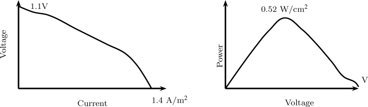
Figure 24.9 An illustrative plot of current density and power density versus voltage in a fuel cell. Temperature = 80 °C, pressure = 2.2 atm. Thampan. T., Malhotra, S. Zhang J and Datta. R; PEM Fuel cell as a membrane reactor, Catalysis Today, Volume 67, 2001.
Voltage decreases as current is increased as expected from the various polarization phenomena in the system. At large currents the voltage drops to almost zero value since the mass transfer resistance clicks in (more of a flowrate limitation in fuel cells). The power density increases at first with an increase in voltage, reaches a maximum, and then starts to fall off with further increase in voltage. The optimum power density is noteworthy and important in determining the optimum operating voltage.
24.8 Li-Ion Battery Modeling
In this section, we discuss briefly the working of a Li-ion battery and the transport steps involved in the system. The discussion in this section is qualitative and the goal is to reiterate the importance of mass transfer processes. In a Li-ion battery, energy is stored by converting electrical energy into chemical energy (specifically by storing lithium in a host material). This is the charging cycle of the battery. During the discharge Li moves from a high energy configuration to a low energy configuration and produces a current that does useful work. Unlike the fuel cell, the battery needs charging and a discharging cycles. Hence transient models are usually implied and steady state models are not applicable.
The process of insertion of lithium into a host is known as intercalation. Graphite is a good host material and Li can be inserted due to the small size of the lithium ions. The insertion material during discharging is usually inorganic metal oxides denoted generally as MO2, where M is a metal atom and is often Co, Mn, or Fe. The two insertion materials are separated by an electrolyte, which facilitates the transport of ions across the two electrolytes. The reactions in the charging and discharging cycles are described briefly next.
24.8.1 Charging
During charging Li ions are released from the anode metal oxide matrix (where they were stored during the discharge cycle). The ions diffuse across the electrolyte and reach the graphite cathode, where they are inserted into the host by the following reaction:
C + xLi+ + xe– → LixC
The transport processes and the reactions during a charging cycle are shown in Figure 24.10. The electrodes are porous and diffusing Li ions undergo a reaction at the carbon surface, picking up electrons from the external power supply. The Li atoms then diffuse into the carbon matrix and occupy host sites within the matrix.

Figure 24.10 Transport and reaction processes taking place during the charging of a Li-ion battery. The cathode matrix gets depleted of Li and the carbon anode gets enriched in Li.
It should be noted that the reaction taking place at the carbon is reduction and that in the Li-loaded metal oxide is oxidation. The electrodes are marked opposite and this can look confusing. The marking is because by convention the electrodes are marked correctly for the discharge cycle, but the name is retained for the charging cycle even though the reactions taking place switch direction during the charging cycle.
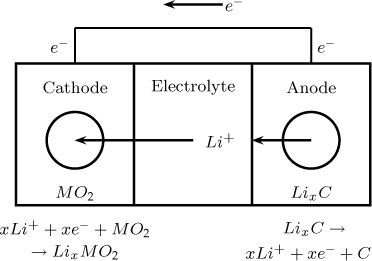
24.8.2 Discharging
The reverse reaction takes place during discharging. Lithium ions are released now from LixC and move to the cathode where they react as
xLi+ + xe– + MO2 → LixMO2
The transport and reaction steps are shown in Figure 24.11.
The transport mechanism were modeled by Jiang and Peng (2016) using time constants for the key transport steps: solution phase diffusion, solid phase diffusion, and charge transport were identified as the limiting phenomena. A transient diffusion reaction model including the migration due to electric field was formulated and solved to simulate the charging and discharging process. Ramadesigan et al. (2012) also provide detailed information on modeling where they use a multiscale modeling approach. The references cited in these two sources are numerous and provide additional resources on modeling of Li-ion batteries. Further details are not provided here due to space limitations.
Summary
Electrochemical processes have a wide range of applications in the energy sector as well as in manufacture of chemicals. In the energy sector, there is a need to store solar energy since this can only be produced during daytime. Battery design becomes therefore an important part of the overall solar energy production industry. Similarly the automobile industry needs large capacity batteries. Fuel cells are central to hydrogen-based energy generation and provide another important application area of electrochemical processes.
An example in the field of chemical production is the production of chlorine and sodium hydroxide by electrolysis of sodium chloride; this precedes the chemical industry. These are large volume chemicals. Other applications can be found in organic synthesis and pharmaceutical production. Adiponitrile production is one of the large-scale applications of electrochemistry for production of organic chemicals.
Analysis of electrochemical systems starts by writing the overall reactions as two half reactions: the anodic reaction where an oxidation is taking place and a cathodic reaction where a reduction takes place. Each reaction is assigned an oxidation potential, which is based on the free energy change of the reaction under standard conditions. The half reactions with negative oxidation potentials are favorable and take place at the anode while the second half reactions become the cathodic reaction since they are favorable in the reverse direction. The overall potential is the sum of the anodic (oxidation) and cathodic (reduction) potentials and represents the minimum voltage needed to carry out the reaction.
If the minimum potential is negative, the reaction is spontaneous and the two half reactions can be used to generate energy. This is the basis of, for example, the hydrogen fuel cell. The absolute value of the minimum potential is called the open circuit voltage and represents the maximum voltage that can be generated in the fuel cell. The maximum voltage applies when zero current is withdrawn from the cell.
The minimum potential applies when the reactants and the products are in standard conditions, usually 1 atm pressure for gases and 1 M solution for liquids. If they are not at standard conditions the Nernst equation is used to correct for the concentration effects.
The difference between the applied electrode potential and the equilibrium potential is defined as the overpotential. An anodic reaction takes place at the electrode if the overpotential is positive and vice versa. The rate of reaction is an exponential function of the overpotential and a kinetic model can be derived based on this concept, which is the Butler-Volmer equation.
The exchange current form of the Butler-Volmer relation is commonly used. The exchange current is actually a kinetic parameter and can be thought of as a measure of the intrinsic activity of the electrode to charge transfer. The values are reported for standard reference concentrations and temperature. These can be corrected to other concentrations using the order of the reaction and to other temperatures using the Arrhenius equation.
The Tafel equation is an inverted form of a simplified Butler-Volmer equation and is often used as an approximate representation of the kinetics of the electrode reactions. The overpotential needed to create a given current can be calculated using this equation if the Tafel constants are known for the given reaction.
Mass transfer rate from the bulk to the electrode surface can be a limiting step and is usually modeled based on film theory, where the migrational contribution is also included (as a correction factor) in addition to the diffusional transport. For fast electrode reactions, the process can be entirely limited by the mass transfer rate and the resulting current is called the limiting current. The concentration drop in the film also causes a difference in potential across the film; this is called the concentration overpotential.
The voltage balance shows how the applied voltage is utilized in various processes in the system: the anode reaction, anode concentration overpotential, solution or membrane drop, cathodic concentration over-potential, cathode reaction, and voltage drop in the external circuit. The applied voltage for an electrochemical process for a given current is calculated from the voltage balance. If the system is a fuel cell, the voltage balance shows how much voltage is actually produced compared to the thermodynamic maximum. Examples provided in the text show the details of these calculations.
A Li-ion battery operates by storage of Li in a “carbon hotel.” The process is known as intercalation. The Li moves from the carbon anode during the discharge cycle where it gets stored within a metal oxide matrix. Once the Li is depleted, the battery is put into a storing cycle where an external power source moves the Li back from the metal oxide to the carbon where it gets stored. Thus the Li-ion batteries are operated in a cycling manner unlike a fuel cell. Modeling requires the application of the Butler-Volmer kinetics, migration effects, and transient solid state diffusion.
Review Questions
24.1 Faraday’s constant is the charge on an electron (C/electron) times the number of electrons per mole. The latter is equal to the Avogadro number. What is the charge on an electron? Using this calculate the value of Faraday’s constant.
24.2 What is meant by a half reaction?
24.3 What reaction (oxidation or reduction) takes place at the anode?
24.4 A current density of 100 A/m2 is measured in a simple single step electrochemical reaction. What is the rate at which the reaction is taking place in mol/m2s?
24.5 What is meant by standard oxidation potential?
24.6 What is meant by standard reduction potential?
24.7 What data is needed to find the overall equilibrium cell potential for an electro-chemical reaction?
24.8 State the Nernst equation for the equilibrium potential.
24.9 When could a pair of half reactions be combined and used as a fuel cell?
24.10 Define the Butler-Volmer equation.
24.11 What is exchange current?
24.12 Define the Tafel equation.
24.13 By what factor is mass transfer enhanced due to electric field? Assume no supporting electrolyte.
24.14 What is the meaning of limiting current?
24.15 What is concentration overpotential?
24.16 What factors are included in the voltage balance?
24.17 When is the power maximum in a fuel cell, at low or high current?
24.18 What is intercalation?
24.19 Describe what happens when a Li-ion battery is charged.
24.20 Describe what happens when a Li-ion battery is being used.
Problems
24.1 Classification of electrode processes. Discuss the engineering issues associated with the four types of electrochemical reactions shown in Figure 24.4. What adjustments in the contacting pattern or design may be appropriate?
24.2 Cu deposition: stoichiometry. Consider the reaction
Cu++ + 2e– → Cu
If the deposition rate is 3 mole/sec find the current flowing through the system. Find the minimum potential needed for the if (impure) copper dissolution is the reaction at the anode. The cathode will be coated with pure copper.
24.3 Open circuit voltage in a hydrogen fuel cell. Find the maximum voltage in a hydrogn fuel cell as a function of oxygen partial pressure and plot the data. Also show the effect of temperature.
24.4 Butler-Volmer equation: thermodynamic consistency. Rearrange Equation 24.9 for zero current and show that it is equivalent to the Nernst relation. Hence verify that the equation is thermodynamically consistent.
24.5 Metal recovery from waste streams. Metal salts are frequently found in waste-water and industral waste streams. These can be electrochemically processed to recover the metals. Thus we not only treat the waste streams but also generate value from waste. The potential for metal recovery and some statistical data are shown in Allen and Rosselot (1997). From their data we see that the metals in many waste streams are significantly underutilized. Thus there is considerable scope for process development and optimum design in this area.
Consider as an example the recovery of Ag from waste, which can be represented by the following overall reaction:
2Ag+ + H20 → 2Ag + 2H+ + 1/2O2
Write this as cathodic and anodic half reactions and find the equilibrium potential for a silver ion concentration of 0.01 M. The actual potential depends on the current density. Assume that at 100 A/m2 the overpotential is 1 V. Find the energy required and compare with the silver cost.
24.6 Cobalt recovery. Cobalt is to be recovered from a solution of cobalt sulfate at a concentration of 0.005 M. Find the reaction potential and also find the potential for the competing reaction of hydrogen evolution at the cathode if the pH of the solution is 1. The standard potential for oxidation of cobalt is 0.277 V.
Note: The reaction potential for hydrogen evolution is 1.17 V at low pH, which is comparable to that for Co deposition. Hence both reactions are likely to occur at this pH. From an application point of view, a relatively high pH is needed for the Co deposition to become the favored reaction. Thus if the wastewater is acidic then Co recovery is difficult using an electrochemical process.
24.7 Parallel plate reactor. A parallel plate reactor is used for deposition of a metal from a solution of concentration 50 mol/m3. The reactor is undivided and has an interelectrode gap of 5 mm and width of 1 m. The electrolyte is supplied with a velocity of 0.1 m/s. Assume a mean current density of 360 A/m2. The electrode kinetics is represented by a Butler-Volmer equation as
i = nF kCM exp( E)
where k = 0.2 and β = 0.5. Find the limiting current. Find the voltage applied and the residence time needed to convert 95% of the metal ion. There is no supporting electrolyte.
24.8 Batch electrochemical mode. A schematic of an electrochemical batch reactor is shown in Figure 24.12 and the goal is to set up a simple model to calculate the batch time. Two modes of operation are to be examined as well.
The first is the potentiostatic mode where the potential difference between the electrode is kept constant. The current will vary with time here. The second is the galvanostatic mode where the current between the electrode is kept constant. The applied voltage will have to vary with time here. Simulate the concentration versus time for an assumed set of parameters, and also show how the current or voltage would vary with time depending on the mode of operation.
24.9 Convection-diffusion model for a parallel plate electrolyzer. A parallel plate electrolyzer can be modeled by a convection-diffusion model. This is particularly suitable for laminar flow and preferred rather than the simple mesoscopic model. The steps in involved are shown in Figure 24.13.

Figure 24.13 Schematic diagram of a parallel plate laminar flow electrolyzer (operated in a continuous mode) showing the three key mass transport steps.
The model is similar to the convection-diffusion model shown in Section 10.1. The migration in the cross-flow direction is an additional term that should be included. The electroneutrality condition provides an additional equation to calculate the electric potential. The boundary condition at the electrode is that flux is equal to i/nF . Set up the model equations and develop a simulation model for this mode of operation.
24.10 Voltage balance in adiponitrile production. Adiponitrile (ADN) is the first major organic chemical to be made by an electrolytic process. The reaction scheme is
Find the free energy change of the reaction and report it as Eeq. Write this as two half reactions. The reaction scheme is complicated, involving both homogeneous and heterogeneous reactions, and a detailed model is given in Suwanvaipattana et al. (2006). In this exercise assume a simple Tafel kinetics for both reactions. Use the following values for the Tafel constants. For water oxidation a = 0.303, b = 0.12 and for acrylonitrile (ACN) conversion a = 0.6, b = 2.2. Perform a voltage balance and plot the results as a current versus voltage curve.