Chapter 12. Convective Mass Transfer in Turbulent Flow

Search in book...
Toggle Font Controls
Create new playlist

Name your new playlist

Playlist description (optional)
Sign In

Email address

Password

Forgot Password?

or

Continue with Facebook

Continue with Google
Sign Up

Full Name

Email address

Confirm Email Address

Password

or

Continue with Facebook

Continue with Google

Chapter 12. Convective Mass Transfer in Turbulent Flow

Learning Objectives

After completing this chapter, you will be able to:

Understand basic properties of turbulent flow and the concept of time averaging.
Appreciate that there is a closure problem in modeling of turbulent flows.
Define and use the eddy diffusivity model for closure of the problem.
Apply the eddy diffusivity model to find the flux and mass transfer coefficients in typical turbulent solid–liquid mass transfer problems.
Understand the basis of the analogy of mass transfer with momentum transfer.
Understand common models of turbulent mass transfer from a gas–liquid interface.

This chapter introduces and solves problems where mass transfer occurs under turbulent flow conditions. We first review some properties of turbulent flow. Turbulent flow is characterized by random velocity fluctuations superimposed on the main flow as well as concentration fluctuations. Hence the flow is always transient in nature. It is difficult to resolve these random fluctuations. To resolve this, the concept of time averaging is introduced, where the time-averaged values are used as representative parameters. The time-averaged form of the convection-diffusion equation for mass transfer and the Navier-Stokes equation for flow are then derived, which forms the starting point of most turbulent transport models.

The averaging introduces additional unknowns known as cross-correlation terms, which have to be closed. This is referred to as the closure problem in turbulent flow analysis. These additional terms can be interpreted as additional transport contributions resulting from the fluctuations. One method of closure is to introduce an eddy viscosity for flow problems and eddy diffusivity for mass transfer problems. These are defined and then used for the solution of illustrative problems in solid–fluid mass transfer in channel flows, pipe flows, and flat plate turbulent boundary layers. A close analogy exists between momentum and mass transfer in such flows and some of the common analogies along with the basis for these are shown.

Turbulent mass transfer from a gas–liquid interface follows a similar approach. Some closure relations based on the eddy diffusivity concept suggested in the literature are reviewed and applied to a problem of mass transfer in turbulent film flow. Overall the chapter provides the necessary background information to follow the more advanced literature in the field and also helps you in understanding the basis of the models that are incorporated into CFD codes for simulation of turbulent transport.

12.1 Properties of Turbulent Flow

Turbulence is the result of flow instability. Any small disturbance could lead to a chaotic type of flow with velocity fluctuating on a small time scale around a mean value. This happens generally when the viscous forces are much smaller than the inertial forces. The viscosity effect stabilizes the flow and dampens any disturbance. In the absence of significant viscous forces, any disturbance persists and leads to a continuous fluctuation of velocity, leading to turbulent flow. Thus turbulent flows are characterized by small random fluctuations around a mean value and essentially are chaotic unsteady state phenomena. The velocity fluctuations cause corresponding fluctuations in concentration for mass transfer problems and in temperature for heat transport situations. Thus the concentration (or temperature in heat transfer problems) fluctuates in a random manner around a mean value.

12.1.1 Transition Criteria

The viscous forces have to be larger than inertial forces for flow to be laminar and these provide a damping effect to any flow disturbance. The relative magnitude of these forces is characterized by a dimensionless group, the Reynolds number:

Reynolds nmber = \frac{Intertia force}{Viscous force}

$Reynolds nmber = \frac{Intertia force}{Viscous force}$

Thus a low Reynolds number means viscous forces are larger than inertial forces and the flow will be laminar. At higher Reynolds numbers the flow becomes turbulent. For pipe flow, the transition Reynolds number is 2100–2300 and the flow is fully turbulent above a Reynolds number of 4000.

For flow in a boundary layer over a flat plate, the transition to turbulence occurs at a Reynolds number of around 2 × 10⁵ and the flow is fully turbulent above 2 × 10⁶. Note that the distance from the leading edge is used in the Reynolds number here and defined as xv_∞ρ/μ.

12.1.2 Characteristics of Fully Turbulent Flow

The flow becomes oscillatory at some critical Reynolds number, which is the onset of instability. Beyond this stage the flow eventually becomes fully turbulent. A fully turbulent flow field has the following characteristics (Warsi, 1999):

Random: The flow field is a random field. For example, two identical experiments may not leave an identical streamline track of a marker particle released at the same position.
Diffusive: The flow disturbance spreads over a larger distance as if it were a diffusion process. A streak of dye released in a pipe under turbulent conditions spreads over the whole pipe.
Dissipative: There is a large energy loss in turbulent flow. For example, the pressure drop has to be increased by 3.5 times in order to double the volumetric flow rate.
Three dimensional: Even a fully developed unidirectional flow (in a time-averaged sense) has some fluctuating velocity components (superimposed on the main flow) in all other three directions.

12.1.3 Stochastic Nature

An important property of turbulent flow is that no two identical experiments give the same velocity profile track, but the statistical properties remain the same. The flow itself may appear steady if the velocity is measured with devices that are not sensitive to small changes (e.g., a pitot tube). The applied pressure drop and the resulting flow rate will be constant in the system in a time-averaged sense (if the system is maintained at constant inlet and outlet pressures). Such flows are called “steady-on-average” in order to distinguish them from turbulent flow, which is inherently transient in nature due to random fluctuations in the velocity. Similarly the concentration at any point will be a constant if measured by sampling the liquid or by probes that are not sensitive to detecting small fluctuations. In engineering analysis these “steady” values are of more interest. Hence it seems logical to look at time-averaged properties of flow rather than the instantaneous velocity versus time profiles. This can be done by a model-reduction procedure called time averaging, discussed next.

12.2 Properties of Time Averaging

In turbulent flow conditions, the instantaneous velocity at any point can be represented as a sum of a mean value and a fluctuating component:

\begin{matrix} υ_{x} (t) = {\bar{υ}}_{x} + {υ x}_{x}^{'} (t) & (12.1) \end{matrix}

$\begin{matrix} υ_{x} (t) = {\bar{υ}}_{x} + {υ x}_{x}^{'} (t) & (12.1) \end{matrix}$

Similar equations hold for the y- and z-directions. The bar indicates a mean or time average of a quantity, which is defined, for example, as

{\bar{υ}}_{x} = \frac{1}{T} \int_{0}^{T} υ_{x} (t) d t

${\bar{υ}}_{x} = \frac{1}{T} \int_{0}^{T} υ_{x} (t) d t$

where T is a sufficiently large value of time for the results to be statistically meaningful. The symbol ′ is used for fluctuating values.

Similarly the concentration (or the temperature) varies in turbulent flow and can be represented as

\begin{matrix} C_{A} (t) = {\bar{C}}_{A} + C_{A}^{'} (t) & (12.2) \end{matrix}

$\begin{matrix} C_{A} (t) = {\bar{C}}_{A} + C_{A}^{'} (t) & (12.2) \end{matrix}$

Here $C_{A}^{'}$ $C_{A}^{'}$ is the fluctuating part of the concentration and ${\bar{C}}_{A}$ ${\bar{C}}_{A}$ is the time-averaged mean value at the given point. The time averaging defined here is a way of modeling the average properties rather than worrying about every minor fluctuation.

Flow and mass transport can be classified into two types depending on whether the time-averaged values change with time or not:

Steady on average case: ${\bar{υ}}_{x}$ ${\bar{υ}}_{x}$ and so on and ${\bar{C}}_{A}$ ${\bar{C}}_{A}$ do not change with time. For example, consider solid dissolution in a pipe. If the inlet flow velocity does not change with time, the time-averaged concentration measured at any point will be found to be constant. Here we assume that the concentration is measured with a device that does not detect small fluctuations, which are characteristics of turbulent flow.
Unsteady on average: If the inlet condition is perturbed, for example, by changing the feed condition, then ${\bar{υ}}_{x}, {\bar{C}}_{A}$ ${\bar{υ}}_{x}, {\bar{C}}_{A}$ , and so on change with time due to these changes in the external conditions. The time scale of these changes is in general relatively large compared to the time scale of fluctuations. Hence the time averaging indicated by, for example, Equation 12.2, can still be used. In particular we will use the property that the time average of any fluctuating quantity is zero. Thus, for example, the time average of $C_{A}^{'}$ $C_{A}^{'}$ is zero.

With this background you should note the following properties of time averaging:

The time average of any fluctuating quantity is zero.
The time average of the product of a time-averaged quantity and fluctuating quantity is zero. Thus, for example, the time average of the product of ${\bar{υ}}_{x}$ ${\bar{υ}}_{x}$ and $υ_{x}^{'}$ $υ_{x}^{'}$ is zero. This rule can be applied for both the steady on average and unsteady on average cases noted previously.
The time average of the product of two fluctuating quantities is non-zero, for example, the time average of the product of $υ_{x}^{'}$ $υ_{x}^{'}$ and $υ_{y}^{'}$ $υ_{y}^{'}$ is non-zero. We say that there is a cross-correlation between $υ_{x}^{'}$ $υ_{x}^{'}$ and $υ_{y}^{'}$ $υ_{y}^{'}$ .

Cross-correlation is an important concept in turbulent flow analysis. If two random variables, say $υ_{x}^{'}$ $υ_{x}^{'}$ and $υ_{y}^{'}$ $υ_{y}^{'}$ , are completely independent then the cross-correlation is zero while if there is some dependency on each other (as is the case is in turbulent flow) then the cross-correlation is non-zero. For instance, the fluctuating components have to satisfy the continuity equation

\frac{\partial υ_{x}^{'}}{\partial x} + \frac{\partial υ_{y}^{'}}{\partial y} = 0

$\frac{\partial υ_{x}^{'}}{\partial x} + \frac{\partial υ_{y}^{'}}{\partial y} = 0$

and hence are therefore interdependent, giving rise to a cross-correlation.

Similarly the cross-correlation average of the product of $υ_{x}^{'}$ $υ_{x}^{'}$ , for instance, and $C_{A}^{'}$ $C_{A}^{'}$ is non-zero. This has important implications in turbulent modeling of mass transfer processes. This is elaborated next and leads to what is known as the closure problem in turbulent flow.

Using these rules we can show that

\bar{υ_{x} C_{A}} = {\bar{υ}}_{x} {\bar{C}}_{A} + \bar{υ_{x}^{'} C_{A}^{'}}

$\bar{υ_{x} C_{A}} = {\bar{υ}}_{x} {\bar{C}}_{A} + \bar{υ_{x}^{'} C_{A}^{'}}$

with similar expressions for the other velocity terms. The first term on the right-hand side is the product of two time-averaged quantities. The second term is the extra term that arises due to cross-correlation. This is the time average of the product of two fluctuating quantities.

Similarly the product of two velocities when time-averaged produces an extra term as indicated in the following:

\bar{υ_{x} υ_{y}} = {\bar{υ}}_{x} {\bar{υ}}_{y} + \bar{υ_{x}^{'} υ_{y}^{'}}

$\bar{υ_{x} υ_{y}} = {\bar{υ}}_{x} {\bar{υ}}_{y} + \bar{υ_{x}^{'} υ_{y}^{'}}$

The extra term on the right-hand side of the above equations can be interpreted as additional transport contributions to the fluctuations. These terms have to be modeled and there is no fundamental way of calculating them. This is referred to as the closure problem in turbulent transport analysis.

12.3 Time-Averaged Equation of Mass Transfer

We show here how the equations of mass transfer are time averaged and how extra terms arise due to time averaging. The equation for mass transfer for the convection-diffusion case is written as

\begin{matrix} \frac{\partial C_{A}}{\partial t} + υ_{x} \frac{\partial C_{A}}{\partial x} + υ_{y} \frac{\partial C_{A}}{\partial y} = - (\frac{\partial J_{A x}}{\partial x} + \frac{\partial J_{A y}}{\partial y}) & (12.3) \end{matrix}

$\begin{matrix} \frac{\partial C_{A}}{\partial t} + υ_{x} \frac{\partial C_{A}}{\partial x} + υ_{y} \frac{\partial C_{A}}{\partial y} = - (\frac{\partial J_{A x}}{\partial x} + \frac{\partial J_{A y}}{\partial y}) & (12.3) \end{matrix}$

The transient terms are retained in turbulent flow. Also the z-terms are not shown to avoid clutter and can be readily added. The diffusion terms are written in flux form for convenience of later interpretation of the turbulent diffusion flux term. These are molecular diffusion terms.

In view of the following continuity condition we have

\frac{\partial υ_{x}}{\partial x} + \frac{\partial υ_{y}}{\partial y} = 0

$\frac{\partial υ_{x}}{\partial x} + \frac{\partial υ_{y}}{\partial y} = 0$

The velocity terms in the concentration equation (Equation 12.3) can be moved into the differential, leading to

\begin{matrix} \frac{\partial C_{A}}{\partial t} + \frac{\partial (υ_{x} C_{A})}{\partial x} + \frac{\partial (υ_{y} C_{A})}{\partial y} = - (\frac{\partial J_{A x}}{\partial x} + \frac{\partial J_{A y}}{\partial y}) & (12.4) \end{matrix}

$\begin{matrix} \frac{\partial C_{A}}{\partial t} + \frac{\partial (υ_{x} C_{A})}{\partial x} + \frac{\partial (υ_{y} C_{A})}{\partial y} = - (\frac{\partial J_{A x}}{\partial x} + \frac{\partial J_{A y}}{\partial y}) & (12.4) \end{matrix}$

Each term is integrated over a chosen period of time (to cover sufficient fluctuations), leading to a time-averaged equation. The bar will be used to denote the time-averaged quantities. All terms with C_A appearing alone can be replaced by the time averaged value since the time average of the fluctuations are zero. This is the consequence of property of time averaging.

However the time average of terms such as υ_xC_A leads to extra terms:

Time average of \frac{\partial (υ_{x} C_{A})}{\partial x} = \frac{\partial (\bar{υ_{x}} \times {\bar{C}}_{A})}{\partial x} + \frac{\partial (\bar{υ_{x}' C_{A}'})}{\partial x}

$Time average of \frac{\partial (υ_{x} C_{A})}{\partial x} = \frac{\partial (\bar{υ_{x}} \times {\bar{C}}_{A})}{\partial x} + \frac{\partial (\bar{υ_{x}' C_{A}'})}{\partial x}$

The second term on the right-hand side is the time average of the product of the velocity fluctuation and the concentration fluctuation. Similar terms appear for the υ_y and υ_z terms. These terms are usually moved to the right-hand side of the equation; the resulting equation is

\begin{matrix} \frac{\partial {\bar{C}}_{A}}{\partial t} + {\bar{υ}}_{x} \frac{\partial {\bar{C}}_{A}}{\partial x} + {\bar{υ}}_{y} \frac{\partial {\bar{C}}_{A}}{\partial y} = - (\frac{\partial J_{A x}}{\partial x} + \frac{\partial J_{A y}}{\partial y}) - \frac{\partial}{\partial x} (\bar{υ_{x}' C_{A}'}) - \frac{\partial}{\partial y} (\bar{υ_{y}' C_{A}'}) & (12.5) \end{matrix}

$\begin{matrix} \frac{\partial {\bar{C}}_{A}}{\partial t} + {\bar{υ}}_{x} \frac{\partial {\bar{C}}_{A}}{\partial x} + {\bar{υ}}_{y} \frac{\partial {\bar{C}}_{A}}{\partial y} = - (\frac{\partial J_{A x}}{\partial x} + \frac{\partial J_{A y}}{\partial y}) - \frac{\partial}{\partial x} (\bar{υ_{x}' C_{A}'}) - \frac{\partial}{\partial y} (\bar{υ_{y}' C_{A}'}) & (12.5) \end{matrix}$

12.3.1 Turbulent Mass Flux

We find extra terms on the right-hand side of Equation 12.5 (last two terms) that can be viewed as contribution of fluctuations to mass transfer. These terms have the appearance of a divergence of a flux vector and hence a turbulent mass flux vector can be defined whose component j is

J_{A, j}^{t} = \bar{C_{A}^{'} υ_{j}^{'}}

$J_{A, j}^{t} = \bar{C_{A}^{'} υ_{j}^{'}}$

Equation 12.5 can then be written as

\begin{matrix} \frac{\partial {\bar{C}}_{A}}{\partial t} + {\bar{υ}}_{x} \frac{\partial {\bar{C}}_{A}}{\partial x} + {\bar{υ}}_{y} \frac{\partial {\bar{C}}_{A}}{\partial y} = - (\frac{\partial J_{A x}}{\partial x} + \frac{\partial J_{A y}}{\partial y}) - \frac{\partial}{\partial x} J_{A, x}^{t} - \frac{\partial}{\partial y} J_{A, y}^{t} & (12.6) \end{matrix}

$\begin{matrix} \frac{\partial {\bar{C}}_{A}}{\partial t} + {\bar{υ}}_{x} \frac{\partial {\bar{C}}_{A}}{\partial x} + {\bar{υ}}_{y} \frac{\partial {\bar{C}}_{A}}{\partial y} = - (\frac{\partial J_{A x}}{\partial x} + \frac{\partial J_{A y}}{\partial y}) - \frac{\partial}{\partial x} J_{A, x}^{t} - \frac{\partial}{\partial y} J_{A, y}^{t} & (12.6) \end{matrix}$

The turbulent flux terms are then added to the molecular flux term (first two terms on the right-hand side) for modeling turbulent mass transfer. These terms have to be modeled and therefore we need some constitutive model for turbulent transport.

12.3.2 Reynolds Stresses

The velocity appearing in the mass transfer model (Equation 12.6) is the time-averaged velocity. In principle it can be computed from the time average of the Navier-Stokes equation. When the N-S equation is averaged extra terms appear; they are represented as turbulent stress tensor. These stresses are also known as Reynolds stresses and are related to the time average of the product of the fluctuating component of velocity. They are defined as

τ_{i j}^{(t)} = - ρ \bar{υ_{i}^{'} υ_{j}^{'}}

$τ_{i j}^{(t)} = - ρ \bar{υ_{i}^{'} υ_{j}^{'}}$

The resulting x-momentum equation upon time averaging of the Navier-Stokes equation is

\begin{matrix} ρ (\frac{\partial ({\bar{υ}}_{x} {\bar{υ}}_{x})}{\partial x} + \frac{\partial ({\bar{υ}}_{x} {\bar{υ}}_{y})}{\partial y}) = - \frac{\partial \bar{P}}{\partial x} + \frac{\partial {\bar{τ}}_{x x}^{(υ)}}{\partial x} + \frac{\partial {\bar{τ}}_{y x}^{(υ)}}{\partial y} + \frac{{\partial τ}_{x x}^{(t)}}{\partial x} + \frac{\partial τ_{y x}^{(t)}}{\partial y} & (12.7) \end{matrix}

$\begin{matrix} ρ (\frac{\partial ({\bar{υ}}_{x} {\bar{υ}}_{x})}{\partial x} + \frac{\partial ({\bar{υ}}_{x} {\bar{υ}}_{y})}{\partial y}) = - \frac{\partial \bar{P}}{\partial x} + \frac{\partial {\bar{τ}}_{x x}^{(υ)}}{\partial x} + \frac{\partial {\bar{τ}}_{y x}^{(υ)}}{\partial y} + \frac{{\partial τ}_{x x}^{(t)}}{\partial x} + \frac{\partial τ_{y x}^{(t)}}{\partial y} & (12.7) \end{matrix}$

The terms in the z-direction are not shown to avoid clutter and can be readily added. Only the x-component of the equation is shown above. Similar expressions hold for the y- and z-components. Also note that in the above equation we have also assumed that the flow is steady on average; hence the time derivative of mean flow is not shown. These equations are known as the RANS (Reynolds-averaged Navier-Stokes) equation.

The extra terms in the RANS equation arise naturally as a consequence of time averaging, but there is no way to predict them. Some extra closure laws are needed; these are discussed in the next section. Before we proceed we show additional coupling that can arise in mass transfer problems with reaction.

12.3.3 Reaction Contribution

For reacting systems, additional contribution to the reaction rate arises due to concentration fluctuations if the reaction is a nonlinear function of concentration. This can be demonstrated by time averaging the reaction terms as shown in the following paragraph.

Consider a second-order reaction with rate R_A defined as $- k_{2} C_{A}^{2}$ $- k_{2} C_{A}^{2}$ . Here C_A is the instantaneous concentration. You should time average this and show that the rate of reaction can be represented as

Rate, time averaged = - (k_{2} {\bar{C}}_{A}^{2} + k_{2} \bar{C_{A}' C_{A}'})

$Rate, time averaged = - (k_{2} {\bar{C}}_{A}^{2} + k_{2} \bar{C_{A}' C_{A}'})$

The first term on the right-hand side is simply the rate based on the time-averaged concentration. The second term is the average of the product of fluctuating concentrations and leads to additional contribution to the rate. This term is non-zero and cannot be calculated. Again we have the closure problem of turbulence for reacting systems (whenever the kinetics are nonlinear). Some phenomenological models are needed at this stage. This is closely related to the macromixing concepts introduced in Chapter 3. See Figure 3.7 as well.

Similar effects can be seen when the reaction rate is expressed as an exponential function of the temperature. Terms of the form $\bar{C_{A}^{'} T'}$ $\bar{C_{A}^{'} T'}$ will appear as additional terms in the rate equation.

12.4 Closure Models

The simplest way to look at the closure is to use some equation similar to Newton’s law of viscosity. Here the turbulent stresses are correlated as a linear function of the mean velocity gradient for 1-D flows (or rate of strain based on mean velocity for 3-D flows). We simply use the analogy with Newton’s law of viscosity and define an eddy diffusivity parameter, ν_t, by the following relation:

\begin{matrix} τ_{y x}^{(t)} = ρ ν_{t} \frac{d {\bar{υ}}_{x}}{d y} & (12.8) \end{matrix}

$\begin{matrix} τ_{y x}^{(t)} = ρ ν_{t} \frac{d {\bar{υ}}_{x}}{d y} & (12.8) \end{matrix}$

for one-dimensional shear type of flows. The parameter introduced, ν_t, is called the kinematic eddy viscosity. Also, the term ρν_t may be viewed as a “turbulent viscosity,” denoted often by μ_t. However, these quantities are property of the flow and not of the fluid. Thus these will be a function of the local Reynolds number, distance from the wall, and so on, and NOT a simple property like viscosity. The closure problem still remains but is now transferred to ν_t or μ_t.

Similarly the mass diffusivity due to turbulent flow is closed by defining a turbulent mass diffusivity parameter, D_t:

\begin{matrix} J_{A, y}^{t} = \bar{C_{A}^{,} υ_{y}^{'}} = - D_{t} \cdot \frac{{\bar{d C}}_{A}}{d y} & (12.9) \end{matrix}

$\begin{matrix} J_{A, y}^{t} = \bar{C_{A}^{,} υ_{y}^{'}} = - D_{t} \cdot \frac{{\bar{d C}}_{A}}{d y} & (12.9) \end{matrix}$

This is for the y-direction with similar definitions for the x- and z-directions. Note that the closure model is similar to Fick’s law.

12.4.1 Turbulent Schmidt Number

Since more data are available on turbulent momentum diffusivity, it is common to scale the turbulent mass diffusivity by scaling by this value. This leads to a parameter, the turbulent Schmidt number:

S c_{t} = \frac{ν_{t}}{D_{t}}

$S c_{t} = \frac{ν_{t}}{D_{t}}$

This is a flow-dependent parameter and not a physical property. A value of 0.9 is commonly used and the problem is closed as an approximation. Thus turbulent diffusivity is assumed to be proportional to eddy momentum diffusivity and is not modeled separately. The idea is that both transports are similar and closely related to each other. Hence data on turbulent flow can be used to calculate the eddy diffusivity.

12.4.2 Prandtl’s Model for Eddy Viscosity

The definition of eddy viscosity does not provide the closure for turbulence since we now need a model for this. It simply transfers the cross-correlation problem to eddy viscosity. The simplest model was provided by Prandtl in 1925 and is even today still widely used. We discuss the model and the resulting equations for eddy viscosity now. Other models are briefly reviewed later.

Prandtl (1925) used an analogy with the kinetic theory of gases to obtain a closure for the eddy viscosity. Fundamental to his theory was the concept of a “mixing length,” denoted usually by l. This is an average length to which an eddy can travel without losing its identity. An eddy can be assumed to retain its momentum up to a distance of l. The (time-averaged) velocity difference between two points separated by a distance l determined using Taylor’s series is

{\bar{υ}}_{x} (y + l) = {\bar{υ}}_{x} (l) + l \frac{d {\bar{υ}}_{x}}{d y}

${\bar{υ}}_{x} (y + l) = {\bar{υ}}_{x} (l) + l \frac{d {\bar{υ}}_{x}}{d y}$

Hence an estimate of the magnitude of the velocity fluctuation is

υ_{x}^{'} \approx \pm l \frac{d {\bar{υ}}_{x}}{d y}

$υ_{x}^{'} \approx \pm l \frac{d {\bar{υ}}_{x}}{d y}$

The ± sign is used since the eddy can move in both the +y and –y directions.

If one assumes that $υ_{y}^{'}$ $υ_{y}^{'}$ is of the same order of magnitude as $υ_{x}^{'}$ $υ_{x}^{'}$ (i.e., turbulence is isotropic or uniform in all directions) then an estimate for the product $υ_{x}^{'} υ_{y}^{'}$ $υ_{x}^{'} υ_{y}^{'}$ can be obtained:

\bar{υ_{x}' υ_{y}'} \approx l \frac{d {\bar{υ}}_{x}}{d y} \cdot l \frac{d {\bar{υ}}_{x}}{d y}

$\bar{υ_{x}' υ_{y}'} \approx l \frac{d {\bar{υ}}_{x}}{d y} \cdot l \frac{d {\bar{υ}}_{x}}{d y}$

Noting that the turbulent shear stress is equal to $ρ \bar{υ_{x}^{'} υ_{y}^{'}}$ $ρ \bar{υ_{x}^{'} υ_{y}^{'}}$ in magnitude, the following equation can be used to represent the turbulent shear stress:

\begin{matrix} τ_{y x}^{(t)} = ρ l^{2} | \frac{d {\bar{υ}}_{x}}{d y} | \frac{d {\bar{υ}}_{x}}{d y} & (12.10) \end{matrix}

$\begin{matrix} τ_{y x}^{(t)} = ρ l^{2} | \frac{d {\bar{υ}}_{x}}{d y} | \frac{d {\bar{υ}}_{x}}{d y} & (12.10) \end{matrix}$

The absolute value is used to fit the sign convention that the stress is positive if the velocity gradient is positive and vice versa.

The mixing length is found to depend linearly on the distance from the wall and the relation is expressed as

l = κy

where κ is a constant (usually taken as 0.4). Hence the turbulent shear stress can also be represented as

\begin{matrix} \begin{matrix} τ_{y x}^{(t)} = ρ κ^{2} y^{2} | \frac{d {\bar{υ}}_{x}}{d y} | \frac{d {\bar{υ}}_{x}}{d y} \end{matrix} & (12.11) \end{matrix}

$\begin{matrix} \begin{matrix} τ_{y x}^{(t)} = ρ κ^{2} y^{2} | \frac{d {\bar{υ}}_{x}}{d y} | \frac{d {\bar{υ}}_{x}}{d y} \end{matrix} & (12.11) \end{matrix}$

The previous equation is known as the Prandtl closure. Comparing Equations 12.8 and 12.11, we have the following closure equation for ν_t:

\begin{matrix} ν_{t} = l^{2} | \frac{d {\bar{υ}}_{x}}{d y} | = κ^{2} y^{2} | \frac{d {\bar{υ}}_{x}}{d y} | & (12.12) \end{matrix}

$\begin{matrix} ν_{t} = l^{2} | \frac{d {\bar{υ}}_{x}}{d y} | = κ^{2} y^{2} | \frac{d {\bar{υ}}_{x}}{d y} | & (12.12) \end{matrix}$

The velocity profile for channel flow, pipe flow, boundary layers, and so on can be calculated using this model. The essential details needed for mass transfer applications are presented in the next section.

12.5 Velocity and Turbulent Diffusivity Profiles

The velocity changes rapidly near the wall in turbulent flow in contrast to laminar flow, where it is a smooth parabolic function. This suggests that different length and velocity scales are needed to make the problem dimensionless. The traditional average velocity and pipe radius used for normalization in laminar flow are not useful in turbulent flow. Detailed analysis (discussed, for example, by Ramachandran, 2013) leads to the following reference velocity:

υ_{r e f} = υ = \sqrt{τ_{ω} / ρ}

$υ_{r e f} = υ = \sqrt{τ_{ω} / ρ}$

υ_f is called the friction velocity. In this definition, τ_w is the wall shear stress.

Similarly the following length scale is suggested:

L_{r e f} = \frac{μ}{ρ υ_{f}}

$L_{r e f} = \frac{μ}{ρ υ_{f}}$

The dimensionless velocity in the flow direction is now defined as $\bar{υ_{x}} / υ_{r e f}$ $\bar{υ_{x}} / υ_{r e f}$ and is denoted as υ⁺. Note that this is a time-averaged velocity. The dimensionless length is defined as y/L_ref and is denoted as y⁺ where y is the distance measured from the wall. The velocity profile of υ⁺ versus y⁺ derived on the basis of the Prandtl eddy viscosity closure are now presented without derivation. These are called universal velocity profiles since they are observed for a wide class of shear driven flows, for examples, pipes, channels, turbulent boundary layers and so on.

12.5.1 Universal Velocity Profiles

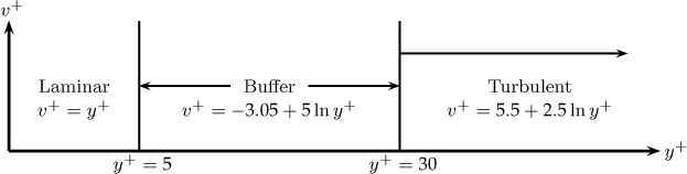
The flow domain in turbulent flow can be divided into three regions: a laminar sublayer also known as viscous layer, a buffer zone, and a turbulent core; velocity profiles are given separately for each of these regions and are as follows:

Near Wall Region: Viscous Sublayer

The turbulence is suppressed near the wall and the flow is laminar in this region. This is known as the laminar sublayer and normally extends to a length equal to 5 when expressed in dimensionless form as y⁺.

The velocity profile in this region is given as

υ⁺ = y⁺ for y⁺ < 5

This equation is found to be valid up to a y⁺ of five, which is called the laminar (viscous) sublayer. This equation can be shown to arise from Newton’s law of viscosity, assuming that the shear stress is nearly constant.

Outside the Viscous Layer: Turbulent Core

Outside the viscous region, usually starting at y⁺ = 30, the flow is mainly turbulent and the laminar contribution to the stress can be neglected. The velocity profile in this region is a logarithmic function of distance and is given as

\begin{matrix} υ^{+} = 2.5 ln y^{+} + 5.5 for y^{+} > 30 & (12.13) \end{matrix}

$\begin{matrix} υ^{+} = 2.5 ln y^{+} + 5.5 for y^{+} > 30 & (12.13) \end{matrix}$

This is called the turbulent core region. This equation can be derived using the Prandtl mixing length model together with some simplifying assumptions.

Buffer Zone

The region in between the laminar layer and the turbulent core, 5 < y⁺ < 30, is called the buffer layer. The velocity here is correlated as

υ⁺ = 5 ln y⁺ – 3.05 for 5 < y⁺ < 30

This is more of a curve fit rather than a model-based equation.

The various regions and the expressions for the corresponding profiles are summarized in Figure 12.1.

Figure 12.1 Illustration of the three regimes for velocity profile equations in turbulent flow.

Velocity Defect near the Center

Equation 12.13 for the fully developed core fits the data well almost up to the center of the channel. At the center the symmetry condition has to be satisfied. that is, dυ⁺/dy⁺ must be zero at y⁺ = H⁺ (the center of the channel or pipe), but it is not as per Equation 12.13. Corrections to account for this error has been suggested and these are in general referred to as the velocity defect law. The error caused by this defect is small for use of these profiles in mass transfer analysis. This is because the concentration change is usually confined to a smaller region near the wall and does not extend all the way to the center of the channel or pipe. However, for study of homogeneous reactions in turbulent flow, this defect can cause errors in overall mass balance and more detailed models for the center region may be warranted in such cases.

12.5.2 Eddy Diffusivity Profiles

For mass transfer analysis, the primary parameter is the mass eddy diffusivity or equivalently the turbulent Schmidt number. We now demonstrate how this parameter can be calculated based on the velocity profiles. For this we need ν_t, the turbulent eddy viscosity, first. It is useful to define a dimensionless total momentum diffusivity as

\begin{matrix} ν_{T}^{+} = \frac{ν + ν_{t}}{ν} = 1 + \frac{ν_{t}}{ν} & (12.14) \end{matrix}

$\begin{matrix} ν_{T}^{+} = \frac{ν + ν_{t}}{ν} = 1 + \frac{ν_{t}}{ν} & (12.14) \end{matrix}$

Note that this is not a physical property and is a turbulence parameter. Thus it varies as a function of y. This parameter is related to the local velocity gradient by the following relationship:

\begin{matrix} ν_{T}^{+} = \frac{1}{(d υ^{+} / d y^{+})} & (12.15) \end{matrix}

$\begin{matrix} ν_{T}^{+} = \frac{1}{(d υ^{+} / d y^{+})} & (12.15) \end{matrix}$

Using this expression the following relations can be obtained by differentiating the velocity profiles for the three regions:

Laminar layer: $ν_{T}^{+} = 1$ $ν_{T}^{+} = 1$ = 1
Buffer layer: $ν_{T}^{+} = 0.2 y^{+}$ $ν_{T}^{+} = 0.2 y^{+}$
Turbulent core: $ν_{T}^{+} = 0.4 y^{+}$ $ν_{T}^{+} = 0.4 y^{+}$

It is also common to define a dimensionless total diffusivity as

D_{T}^{+} = \frac{D + D_{t}}{D}

$D_{T}^{+} = \frac{D + D_{t}}{D}$

This is related to the turbulent Schmidt number Sc_t by

\begin{matrix} D_{T}^{+} = 1 + \frac{S c}{S c_{t}} (ν_{T}^{+} - 1) & (12.16) \end{matrix}

$\begin{matrix} D_{T}^{+} = 1 + \frac{S c}{S c_{t}} (ν_{T}^{+} - 1) & (12.16) \end{matrix}$

Thus if the turbulent Schmidt number is assigned some value, then $D_{T}^{+}$ $D_{T}^{+}$ and correspondingly the turbulent diffusivity D_t can be estimated. The value of 0.9 is usually assigned for the turbulent Schmidt number.

12.5.3 Wall Shear Stress Relations

It should be noted here that the wall shear stress is needed as a primary parameter to complete these calculations (since it was used to scale the velocity and the length). A commonly used equation for this is summarized here from the fluid mechanics literature. The wall shear stress is correlated to the friction factor for internal flows:

τ_{w} = f \frac{ρ 〈 υ 〉^{2}}{2}

$τ_{w} = f \frac{ρ 〈 υ 〉^{2}}{2}$

where 〈υ〉 is the average velocity in the pipe. The friction factor in turn is correlated empirically as a function of the Reynolds number and the following correlation is commonly used for pipe flows (a number of other correlations are available):

f = \frac{0.0 791}{R e^{1 / 4}}

$f = \frac{0.0 791}{R e^{1 / 4}}$

This is commonly used for smooth pipes. Similar correlations are available for rough pipes (see for example in the book by Welty et al., 2008).

For external flow the wall shear stress is known if the drag coefficient is known, and they are related by the following equation:

τ_{ω} = C_{f x} \frac{ρ υ_{e}^{2}}{2}

$τ_{ω} = C_{f x} \frac{ρ υ_{e}^{2}}{2}$

Here υ_e is the velocity in the external flow, that is, at the edge of the boundary layer. The local drag coefficient in turbulent external flow is correlated as

C_{f x} = \frac{0.0 576}{R e_{x}^{1 / 5}}

$C_{f x} = \frac{0.0 576}{R e_{x}^{1 / 5}}$

With this background we can examine turbulent mass transfer in channel flow and pipe flows. Again some further approximations are needed so that simple analytical solutions can be obtained. More complete analysis requires a numerical solution. The analysis is first done for gases where the molecular Schmidt numbers are on the order of one. For liquids. a modified analysis is useful since most of the concentration drop occurs mostly near the wall due to the large value of the Schmidt number.

12.6 Turbulent Mass Transfer in Channels and Pipes

The convection-diffusion equation of mass transfer in a channel under turbulent flow conditions can be represented for the time averaged value as

\begin{matrix} {\bar{υ}}_{x} (y) \frac{\partial \bar{C_{A}}}{\partial x} = - \frac{\partial}{\partial y} (J_{y}^{(m)} + J_{y}^{(t)}) & (12.17) \end{matrix}

$\begin{matrix} {\bar{υ}}_{x} (y) \frac{\partial \bar{C_{A}}}{\partial x} = - \frac{\partial}{\partial y} (J_{y}^{(m)} + J_{y}^{(t)}) & (12.17) \end{matrix}$

The main difference between this and the laminar flow is the inclusion of the extra term (last term) arising from turbulent fluctuations, the so-called eddy mass flux term. Also, the velocity is the time-averaged value. Appropriate boundary conditions are applied at the channel walls. A similar equation can be formulated for pipe flows and the resulting problem is often referred to as the turbulent Graetz problem. The concentration profile in the turbulent boundary layer for mass transfer from a plate, for example, follows a similar model.

In general this problem requires a numerical solution and a number of studies (e.g., Larson and Verazunis, 1973) have addressed this approach. Here a simpler approach is presented where the concentration variation only in the cross-flow direction is considered. This approach involves some simplifications to the preceding differential equation. But this is adequate to predict the wall mass transfer coefficient and is therefore widely used in engineering practice. The simplified model is now presented.

12.6.1 Simplified Analysis: Constant Wall Flux

We analyze here the problem under conditions of constant wall mass flux J_w. Since the variation of concentration in the y-direction is more significant, we make a simplifying assumption that the mass flux varies linearly in the y-direction. This means that the convective term (left-hand side) of Equation 12.17 is simply assumed to be a constant. This assumption of a linear variation of the total mass flux, J_y, with y can be represented as

J_{y} = J_{y}^{(m)} + J_{y}^{(t)} = J_{w} (1 - y / H)

$J_{y} = J_{y}^{(m)} + J_{y}^{(t)} = J_{w} (1 - y / H)$

where J_w is the mass flux at the wall.

The molecular term is written using the Schmidt number, Sc, as

\begin{matrix} J_{y}^{(m)} = - D \frac{d {\bar{C}}_{A}}{d y} = - \frac{ν}{S c} \frac{d {\bar{C}}_{A}}{d y} & (12.18) \end{matrix}

$\begin{matrix} J_{y}^{(m)} = - D \frac{d {\bar{C}}_{A}}{d y} = - \frac{ν}{S c} \frac{d {\bar{C}}_{A}}{d y} & (12.18) \end{matrix}$

The turbulent term is written using the turbulent Schmidt number, Sc_t, as

\begin{matrix} J_{y}^{(t)} = - D_{t} \frac{d {\bar{C}}_{A}}{d y} = - \frac{ν_{t}}{S c_{t}} \frac{d {\bar{C}}_{A}}{d y} & (12.19) \end{matrix}

$\begin{matrix} J_{y}^{(t)} = - D_{t} \frac{d {\bar{C}}_{A}}{d y} = - \frac{ν_{t}}{S c_{t}} \frac{d {\bar{C}}_{A}}{d y} & (12.19) \end{matrix}$

ν_t is equal to $ν (ν_{T}^{+} - 1)$ $ν (ν_{T}^{+} - 1)$ where $ν_{T}^{+}$ $ν_{T}^{+}$ is the dimensionless total momentum diffusivity. Hence the turbulent mass is represented as

\begin{matrix} J_{y}^{(t)} = - ν \frac{(ν_{T}^{+} - 1)}{S c_{t}} \frac{d {\bar{C}}_{A}}{d y} & (12.20) \end{matrix}

$\begin{matrix} J_{y}^{(t)} = - ν \frac{(ν_{T}^{+} - 1)}{S c_{t}} \frac{d {\bar{C}}_{A}}{d y} & (12.20) \end{matrix}$

The total flux can be written as

\begin{matrix} - ν (\frac{1}{S c} + \frac{ν_{T}^{+} - 1}{S c_{t}}) \frac{d {\bar{C}}_{A}}{d y} = J_{w} (1 - y / H) & (12.21) \end{matrix}

$\begin{matrix} - ν (\frac{1}{S c} + \frac{ν_{T}^{+} - 1}{S c_{t}}) \frac{d {\bar{C}}_{A}}{d y} = J_{w} (1 - y / H) & (12.21) \end{matrix}$

Let us introduce the dimensionless distance y⁺ here. Recall that this was defined as y⁺ = yρυ_f/μ = yυ_f/ν.

Hence Equation 12.21 can be written as

\begin{matrix} - υ f (\frac{1}{S c} + \frac{ν_{T}^{+} - 1}{S c_{t}}) \frac{d {\bar{C}}_{A}}{d y^{+}} = J_{w} (1 - \frac{y^{+}}{H +}) & (12.22) \end{matrix}

$\begin{matrix} - υ f (\frac{1}{S c} + \frac{ν_{T}^{+} - 1}{S c_{t}}) \frac{d {\bar{C}}_{A}}{d y^{+}} = J_{w} (1 - \frac{y^{+}}{H +}) & (12.22) \end{matrix}$

This calls for a dimensionless (time-averaged) concentration $c_{A}^{+}$ $c_{A}^{+}$ , which should be defined as

\begin{matrix} c_{A}^{+} = (C_{A s} - {\bar{C}}_{A}) υ_{f} / J_{w} & (12.23) \end{matrix}

$\begin{matrix} c_{A}^{+} = (C_{A s} - {\bar{C}}_{A}) υ_{f} / J_{w} & (12.23) \end{matrix}$

to simplify the model representation. Also, $c_{A}^{+}$ $c_{A}^{+}$ is zero when y⁺ is zero. H⁺ is the dimensionless width of the channel, defined as H/L_ref , which is equal to Hυ_fρ/μ; this has the same grouping as the Reynolds number.

Using the above definition of the dimensionless concentration, Equation 12.22 is written as

\begin{matrix} (\frac{1}{S c} + \frac{ν_{T}^{+} - 1}{S c_{t}}) \frac{d c_{A}^{+}}{d y^{+}} = (1 - \frac{y^{+}}{H +}) & (12.24) \end{matrix}

$\begin{matrix} (\frac{1}{S c} + \frac{ν_{T}^{+} - 1}{S c_{t}}) \frac{d c_{A}^{+}}{d y^{+}} = (1 - \frac{y^{+}}{H +}) & (12.24) \end{matrix}$

The integrated form of the above equation is

\begin{matrix} \begin{matrix} c_{A}^{+} = \int_{0}^{y^{+}} \frac{(1 - y^{+} / H^{+})}{1 / S c + (1 / S c_{t}) (ν_{T}^{+} - 1)} d y^{+} \end{matrix} & (12.25) \end{matrix}

$\begin{matrix} \begin{matrix} c_{A}^{+} = \int_{0}^{y^{+}} \frac{(1 - y^{+} / H^{+})}{1 / S c + (1 / S c_{t}) (ν_{T}^{+} - 1)} d y^{+} \end{matrix} & (12.25) \end{matrix}$

This is the formal representation to calculate the concentration distribution. If a model for $ν_{T}^{+}$ $ν_{T}^{+}$ and for Sc_t as a function of y is proposed, the above equation can be integrated to find the concentration profiles.

Solution for Different Regions

It is convenient to integrate Equation 12.25 for each region separately. Also, the term (1 – y⁺/H⁺) is often taken as 1 for simplification. This assumption certainly holds near the walls where most of the concentration changes occur. Hence Equation 12.25 is simplified as

\begin{matrix} c_{A}^{+} = \int_{0}^{y^{+}} \frac{d y^{+}}{1 / S c + (1 / S c_{t}) (ν_{T}^{+} - 1)} & (12.26) \end{matrix}

$\begin{matrix} c_{A}^{+} = \int_{0}^{y^{+}} \frac{d y^{+}}{1 / S c + (1 / S c_{t}) (ν_{T}^{+} - 1)} & (12.26) \end{matrix}$

This may not be good near the center but the effect of this “center defect” on the calculation of wall mass flux and the Sherwood number is generally small. The solution for $c_{A}^{+}$ $c_{A}^{+}$ for three regions (laminar, buffer, and turbulent) will now be presented.

Near Wall Region: Viscous Sublayer

Here ν_t is small and therefore $ν_{T}^{+} = 1$ $ν_{T}^{+} = 1$ . Hence Equation 12.26 simplified and it is easy to show that the concentration profile in the viscous region is

\begin{matrix} c_{A}^{+} = S c y^{+} & (12.27) \end{matrix}

$\begin{matrix} c_{A}^{+} = S c y^{+} & (12.27) \end{matrix}$

This is valid for y⁺ < 5. Note that the (dimensionless) concentration profile is now scaled by Sc.

Since υ⁺ = y⁺ we find

\begin{matrix} c_{A}^{+} = S c υ^{+} & (12.28) \end{matrix}

$\begin{matrix} c_{A}^{+} = S c υ^{+} & (12.28) \end{matrix}$

and if $S c = 1, c_{A}^{+}$ $S c = 1, c_{A}^{+}$ is the same as υ⁺, which justifies the Reynolds analogy.

Buffer Zone

The region between the laminar layer and the turbulent core, 5 < y⁺ < 30, is called the buffer layer. The velocity here was correlated as

υ⁺ = 5 ln y⁺ – 3.05

Differentiation of this gives an expression for $ν_{T}^{+}$ $ν_{T}^{+}$ ; it was shown earlier that

ν_{T}^{+} = 0.2 y^{+}

$ν_{T}^{+} = 0.2 y^{+}$

for the above velocity profile. Hence the formal expression for the concentration profile is

\begin{matrix} c_{A}^{+} - 5 S c = \int_{5}^{y^{+}} \frac{d y^{+}}{1 / S c + (1 / S c_{t}) (0.2 y^{+} - 1)} & (12.29) \end{matrix}

$\begin{matrix} c_{A}^{+} - 5 S c = \int_{5}^{y^{+}} \frac{d y^{+}}{1 / S c + (1 / S c_{t}) (0.2 y^{+} - 1)} & (12.29) \end{matrix}$

The value of Sc_t in the buffer zone is taken as one. Using this value and integrating, we obtain

\begin{matrix} c_{A}^{+} = 5 S c + 5 ln [S c [(y^{+} / 5) - 1] + 1] & (12.30) \end{matrix}

$\begin{matrix} c_{A}^{+} = 5 S c + 5 ln [S c [(y^{+} / 5) - 1] + 1] & (12.30) \end{matrix}$

The value of $c_{A}^{+}$ $c_{A}^{+}$ at the edge of the buffer zone (at a y⁺ of 30) is

\begin{matrix} c_{A}^{+} (30) = 5 S c + 5 ln (5 S c + 1) & (12.31) \end{matrix}

$\begin{matrix} c_{A}^{+} (30) = 5 S c + 5 ln (5 S c + 1) & (12.31) \end{matrix}$

which is needed as the integration constant for the next step.

Turbulent Core

Here the velocity profile in the turbulent core is given as

\begin{matrix} υ^{+} = 2.5 ln y^{+} + 5.5 & (12.32) \end{matrix}

$\begin{matrix} υ^{+} = 2.5 ln y^{+} + 5.5 & (12.32) \end{matrix}$

which is found to be valid for y⁺ > 30. This is called the turbulent core region. Differentiating this, we represent $ν_{T}^{+}$ $ν_{T}^{+}$ as 0.4y⁺ as shown earlier. Also, Sc_t is taken as 0.9. Further, 1/Sc – 1/Sc_t is much smaller than $ν_{T}^{+} / S c_{t}$ $ν_{T}^{+} / S c_{t}$ , and this term can be neglected. Hence the integral for the concentration profile in the turbulent core in Equation 12.6 simplifies to

\begin{matrix} c_{A}^{+} - c_{A}^{+} (a t y^{+} = 30) = \int_{30}^{y^{+}} \frac{d y^{+}}{(1 / 0.9) (0.4 y^{+})} & (12.33) \end{matrix}

$\begin{matrix} c_{A}^{+} - c_{A}^{+} (a t y^{+} = 30) = \int_{30}^{y^{+}} \frac{d y^{+}}{(1 / 0.9) (0.4 y^{+})} & (12.33) \end{matrix}$

Integrating and using Equation 12.31 for c_A at y⁺ = 30, the concentration profile in the turbulent core is obtained as

\begin{matrix} c_{A}^{+} = 5 S c + 5 ln (5 S c + 1) + 2.2 5 ln (y^{+} / 30) & (12.34) \end{matrix}

$\begin{matrix} c_{A}^{+} = 5 S c + 5 ln (5 S c + 1) + 2.2 5 ln (y^{+} / 30) & (12.34) \end{matrix}$

where the factor 2.25 arises from Sc_t/0.4, which is equal to 0.9/0.4 = 2.25.

The concentration profile has a discontinuity in the slope at the edge of the turbulent core. Also, ${d c}_{A}^{+} / d y^{+}$ ${d c}_{A}^{+} / d y^{+}$ does not reach zero at y⁺ = H⁺, that is, at the center. But these are not considered to be of great concern in the predictions of mass transfer coefficients.

The results for the concentration profile shown for the channel flow are also applicable to pipe flow with y defined as the distance from the wall as well as for turbulent boundary layers. We now demonstrate the use of this to derive an expression for the calculation of the Stanton number.

12.6.2 Stanton Number Calculation for Boundary Layers

Using the expression for the concentration profile and its gradient, an expression for the mass transfer coefficient can be developed. Note that C_As – C_A∞ is used as the driving force for external flows and hence

k_m = J_w/(C_As – C_A∞∞)

This is represented usually in terms of the Stanton number, defined as k_m/_v∞. Now, using the definition of dimensionless concentration defined by Equation 12.23, the local Stanton number can be shown to be related to the drag coefficient as

\begin{matrix} S t_{x} = (\frac{C_{f x}}{2})^{1 / 2} \frac{1}{c_{A e}^{+}} & (12.35) \end{matrix}

$\begin{matrix} S t_{x} = (\frac{C_{f x}}{2})^{1 / 2} \frac{1}{c_{A e}^{+}} & (12.35) \end{matrix}$

where $c_{A e}^{+}$ $c_{A e}^{+}$ is the dimensionless concentration at the edge of the boundary layer. This is defined as

\begin{matrix} c_{A e}^{+} = (C_{A s} - C_{A \infty}) υ_{f} / J_{w} & (12.36) \end{matrix}

$\begin{matrix} c_{A e}^{+} = (C_{A s} - C_{A \infty}) υ_{f} / J_{w} & (12.36) \end{matrix}$

The expression for $c_{A e}^{+}$ $c_{A e}^{+}$ can be obtained by applying Equation 12.34 at y = δ or correspondingly at y⁺ = δ ⁺. The latter is in turn related to $υ_{e}^{+}$ $υ_{e}^{+}$ , which is in turn related to the drag coefficient. The resulting expression for $c_{A e}^{+}$ $c_{A e}^{+}$ after some algebra (which is left as an exercise problem) is

\begin{matrix} c_{A e}^{+} = 5 S c + 5 ln (5 S c + 1) + S c_{t} [\sqrt{2 / C_{f x}} - 14] & (12.37) \end{matrix}

$\begin{matrix} c_{A e}^{+} = 5 S c + 5 ln (5 S c + 1) + S c_{t} [\sqrt{2 / C_{f x}} - 14] & (12.37) \end{matrix}$

Note that the factor 2.25 in 12.34 is equal to Sc_t/0.4, which is used in getting to this form; Sc_t = 0.9 is used here.

Substituting in the local Stanton number expression from Equation 12.35, we have

\begin{matrix} S t_{x} = \frac{\sqrt{C_{f x} / 2}}{5 S c + 5 ln (5 S c + 1) + S c_{t} [\sqrt{2 / C_{f x}} - 14]} & (12.38) \end{matrix}

$\begin{matrix} S t_{x} = \frac{\sqrt{C_{f x} / 2}}{5 S c + 5 ln (5 S c + 1) + S c_{t} [\sqrt{2 / C_{f x}} - 14]} & (12.38) \end{matrix}$

The denominator can be viewed as the sum of three resistances in series, the viscous sublayer, the buffer region, and the fully developed turbulent core. The relative magnitude of these will depend on the molecular Prandtl number and the Reynolds number. The equation is a good representation of data for 0.5 < Sc < 30.

Equation 12.38 can be rearranged to

\begin{matrix} S t_{x} = \frac{C_{f x} / 2}{S c_{t} + 5 \sqrt{C_{f x} / 2} [S c + ln (5 S c + 1) - 14 S c_{t} / 5]} & (12.39) \end{matrix}

$\begin{matrix} S t_{x} = \frac{C_{f x} / 2}{S c_{t} + 5 \sqrt{C_{f x} / 2} [S c + ln (5 S c + 1) - 14 S c_{t} / 5]} & (12.39) \end{matrix}$

This form is easier to compare with the various analogies proposed between momentum and heat transfer. We now illustrate the various analogies proposed in the literature and show that these arise as special cases of the above equation.

12.6.3 Analogy with Momentum Transfer

The simplest is the Reynolds analogy, which states that

S t_{x} = \frac{C_{f x}}{2}

$S t_{x} = \frac{C_{f x}}{2}$

Comparing with Equation 12.39, we find that this holds if Sc = 1, and Sc_t = 1, since the denominator can be shown be equal to one for these values.

Then there is the Prandtl analogy. This follows from Equation 12.39 by setting Sc_t equal to one:

\begin{matrix} S t_{x} = \frac{C_{f x} / 2}{1 + 5 \sqrt{C_{f x} / 2} [S c - 1]} & (12.40) \end{matrix}

$\begin{matrix} S t_{x} = \frac{C_{f x} / 2}{1 + 5 \sqrt{C_{f x} / 2} [S c - 1]} & (12.40) \end{matrix}$

The von Karman analogy is obtained by setting Sc_t = 0.9, and is shown next:

\begin{matrix} S t_{x} = \frac{C_{f x} / 2}{1 + 5 \sqrt{C_{f x}} [S c - 1 + ln (1 + 5 (S c - 1) / 6]} & (12.41) \end{matrix}

$\begin{matrix} S t_{x} = \frac{C_{f x} / 2}{1 + 5 \sqrt{C_{f x}} [S c - 1 + ln (1 + 5 (S c - 1) / 6]} & (12.41) \end{matrix}$

All the analogies differ only in the way the denominator term in Equation 12.39 is handled and what value is assigned to Sc_t.

Role of Molecular Sc

For the larger Sc case the mass transfer boundary layer is very thin and can be buried within the laminar sublayer and the buffer region. The thickness of the order of 15/Sc^1/3 is considered to be an indicative magnitude of this region. The velocity profile in these regions affect the mass transport rate significantly for this case. Hence, a more accurate value of velocity profile in the buffer region and also in the viscous region may be needed. A modified equation is suggested in Section 12.7 where the von Karman profile for velocity (rather than the Prandtl profile with υ⁺ = y⁺) is used.

Role of Turbulent Sc

A second point of caution is the value assigned to Sc_t. A constant value of 0.9 is usually assigned but it appears from the literature that a value that depends on the Re is more realistic. One explanation is that as Re is increased the turbulent energy spectrum moves to larger eddies, which may not be contributing in an equally proportional manner to mass transfer. A survey of various methods for assigning a proper value to Sc_t has been reviewed by Combest et al. (2011). For a further study of this topic this paper may be useful.

12.6.4 Stanton Number for Pipe Flows

The calculation of the Stanton number for pipe flow is similar but the difference is that the cup-mixing concentration rather than the external concentration should be used in the driving force. Thus the definition of mass transfer coefficient is

J_w = k_m(C_As – C_Ab)

where C_Ab is the average concentration in the pipe (at any given axial location) and hence the Stanton number (k_m/ < υ >) can be shown to be

\begin{matrix} S t = \sqrt{\frac{f}{2}} \cdot \frac{1}{c_{A b}^{+}} & (12.42) \end{matrix}

$\begin{matrix} S t = \sqrt{\frac{f}{2}} \cdot \frac{1}{c_{A b}^{+}} & (12.42) \end{matrix}$

which is an expression similar to that for the boundary layer (Equation 12.35). Here f is the friction factor. However $c_{A b}^{+}$ $c_{A b}^{+}$ is an integral of the concentration profile and is formally given in terms of dimensionless variables as

\begin{matrix} c_{A b}^{+} = \frac{2}{υ_{b}^{+} (R^{+})^{2}} \int_{0}^{1} υ^{+} c_{A}^{+} (R^{+} - y^{+}) d y^{+} & (12.43) \end{matrix}

$\begin{matrix} c_{A b}^{+} = \frac{2}{υ_{b}^{+} (R^{+})^{2}} \int_{0}^{1} υ^{+} c_{A}^{+} (R^{+} - y^{+}) d y^{+} & (12.43) \end{matrix}$

In practice, it is difficult to estimate $c_{A b}^{+}$ $c_{A b}^{+}$ . Note numerical integration can be done using Equation 12.43 if detailed υ⁺ and $C_{A}^{+}$ $C_{A}^{+}$ profiles are computed. But it is easy to find $c_{A c}^{+}$ $c_{A c}^{+}$ , the dimensionless center concentration, by simple substitution in the concentration profile expression for the turbulent core region. Hence St is expressed as

S t = \sqrt{\frac{f}{2}} (\frac{c_{A c}^{+}}{c_{A b}^{+}}) (\frac{1}{c_{A c}^{+}})

$S t = \sqrt{\frac{f}{2}} (\frac{c_{A c}^{+}}{c_{A b}^{+}}) (\frac{1}{c_{A c}^{+}})$

From the expressions derived earlier (Equation 12.34), the dimensionless center concentration is easily obtained:

c_{A c}^{+} = 5 S c + 5 ln (5 S c + 1) + 2.2 5 ln (R^{+} / 30)

$c_{A c}^{+} = 5 S c + 5 ln (5 S c + 1) + 2.2 5 ln (R^{+} / 30)$

Since $R^{+} = Re / (2 υ_{b}^{+}) = Re \sqrt{f / 2} / 2$ $R^{+} = Re / (2 υ_{b}^{+}) = Re \sqrt{f / 2} / 2$ , this can be expressed as

c_{A c}^{+} = 5 S c + 5 ln (5 s c + 1) + 2.2 5 ln (R e \sqrt{f / 2} / 60)

$c_{A c}^{+} = 5 S c + 5 ln (5 s c + 1) + 2.2 5 ln (R e \sqrt{f / 2} / 60)$

Hence the Stanton number is given as

\begin{matrix} S t = \frac{c_{A c}^{+}}{c_{A b}^{+}} \cdot \frac{\sqrt{f / 2}}{5 S c + 5 ln (5 S c + 1) + 2.2 5 ln (R e \sqrt{f / 2} / 60)} & (12.44) \end{matrix}

$\begin{matrix} S t = \frac{c_{A c}^{+}}{c_{A b}^{+}} \cdot \frac{\sqrt{f / 2}}{5 S c + 5 ln (5 S c + 1) + 2.2 5 ln (R e \sqrt{f / 2} / 60)} & (12.44) \end{matrix}$

The first term $c_{A c}^{+} / c_{A b}^{+}$ $c_{A c}^{+} / c_{A b}^{+}$ is usually close to unity in turbulent flow due to the fact that the concentration profiles are flatter in the turbulent case than the laminar case and confined more closely to the wall region. This term is therefore approximated as one as a further approximation. (Note: A correction factor for the center to bulk concentration ratio can be developed, see, for instance, Mills, 1993).

Hence Equation 12.44 for the Stanton number is simplified as

\begin{matrix} S t = \frac{\sqrt{f / 2}}{5 S c + 5 ln (5 S c + 1) + 2.2 5 ln (R e \sqrt{f / 2}) / 60)} & (12.45) \end{matrix}

$\begin{matrix} S t = \frac{\sqrt{f / 2}}{5 S c + 5 ln (5 S c + 1) + 2.2 5 ln (R e \sqrt{f / 2}) / 60)} & (12.45) \end{matrix}$

This expression relates the Stanton number (a measure of mass transfer) to the friction factor (a measure of momentum transfer) and is another example of the analogies used in mass transfer.

These models are particularly good compared to experimental data for gases and useful for Sc < 30 or so. For large Sc fluids the mass transfer boundary layer is rather thin and a slightly modified treatment described in the following section is used.

12.7 Van Driest Model for Large Sc

In the treatment of mass transfer in turbulent liquid flow an additional complication arises for mass transfer in liquids where the Sc can be as high as 1000! Here the concentration gradients are confined mostly to the viscous layer and to some extent to the buffer zone and any error in the velocity profile in this region will affect the predictions considerably. We illustrate the difference by looking at alternative models for mixing length near the wall.

It can be shown that the eddy viscosity varies as y³ rather than as y² as per the Prandtl mixing length model (exercise problem 7). This can be accommodated by a more precise form of l, the mixing length. One such model was suggested by van Driest (1956), who proposed a simple exponential damping factor for l:

\begin{matrix} l = κ y [1 - exp (- \frac{y^{+}}{26})] & (12.46) \end{matrix}

$\begin{matrix} l = κ y [1 - exp (- \frac{y^{+}}{26})] & (12.46) \end{matrix}$

This permits a smooth transition from the viscous layer to the turbulent core without the need to introduce an artificial buffer zone. This is one of many equations suggested for the near wall region and many improvements have been suggested. For example, Cebeci and Smith (1974) proposed that the constant 26.0 should be replaced by a function of dimensionless quantities involving factors such as pressure gradients, mass transfer rate, fluid compressibility, and other factors. Note that the van Driest model predicts the cube variation of the eddy viscosity near the wall.

A modified van Driest equation has also been proposed by Hanna et al. (1981). According to their model a denominator term is added to the original van Driest model:

\begin{matrix} l = κ y \frac{[1 - exp (- y^{+} / 26)]}{\sqrt{1 - exp (- 026 y^{+})}} & (12.47) \end{matrix}

$\begin{matrix} l = κ y \frac{[1 - exp (- y^{+} / 26)]}{\sqrt{1 - exp (- 026 y^{+})}} & (12.47) \end{matrix}$

This expression also predicts the correct behavior that the turbulent viscosity will be proportional to y³ near the wall. Taking the limit as y → 0, the eddy viscosity near the wall can be represented as

\begin{matrix} ν_{t} = ν (\frac{y^{+}}{C})^{3} & (12.48) \end{matrix}

$\begin{matrix} ν_{t} = ν (\frac{y^{+}}{C})^{3} & (12.48) \end{matrix}$

where C includes all the constant terms in the modified model. An adjusted value of 14.5 is assigned to this based on experimental results. The relation for mass transfer coefficient based on the modified van Driest model is now examined.

The mass flux is given by

\begin{matrix} J_{A} = - (D + ν_{t} / S c_{t}) \frac{d C_{A}}{d y} & (12.49) \end{matrix}

$\begin{matrix} J_{A} = - (D + ν_{t} / S c_{t}) \frac{d C_{A}}{d y} & (12.49) \end{matrix}$

where Sc_t is the turbulent Schmidt number. Note that ν_t/Sc_t is equal to D_t, the turbulent diffusivity.

The flux J_A is assumed to be a constant equal to wall mass flux J_Aw in the boundary layer.

We also introduce a dimensionless total momentum diffusivity as done earlier:

\begin{matrix} ν_{T}^{+} = 1 + \frac{ν_{t}}{ν} & (12.50) \end{matrix}

$\begin{matrix} ν_{T}^{+} = 1 + \frac{ν_{t}}{ν} & (12.50) \end{matrix}$

Equation 12.49 can now be expressed as

\begin{matrix} \frac{J_{A w}}{ν} = - [\frac{1}{S c} + \frac{(1}{S c_{t}} (ν_{T}^{+} - 1)] \frac{d C_{A}}{d y} & (12.51) \end{matrix}

$\begin{matrix} \frac{J_{A w}}{ν} = - [\frac{1}{S c} + \frac{(1}{S c_{t}} (ν_{T}^{+} - 1)] \frac{d C_{A}}{d y} & (12.51) \end{matrix}$

Dimensionless length y⁺ = y(τ_w/ρ)^1/2/ν is also introduced and Equation 12.51 can be formally integrated across the boundary layer to obtain an expression relating the wall mass flux and the wall shear stress:

\begin{matrix} (\sqrt{τ_{w} / ρ}) \frac{C_{A \infty} - C_{A s}}{J_{A W}} = \int_{0}^{δ +} \frac{1}{1 / S c + (1 / S c_{t}) (ν_{T}^{+} - 1)} d y^{+} & (12.52) \end{matrix}

$\begin{matrix} (\sqrt{τ_{w} / ρ}) \frac{C_{A \infty} - C_{A s}}{J_{A W}} = \int_{0}^{δ +} \frac{1}{1 / S c + (1 / S c_{t}) (ν_{T}^{+} - 1)} d y^{+} & (12.52) \end{matrix}$

The relation $τ_{ω} = C_{f x} ρ υ_{e}^{2} / 2$ $τ_{ω} = C_{f x} ρ υ_{e}^{2} / 2$ is now used. Further, the mass transfer coefficient is expressed terms of the Stanton number by the following relation:

\frac{J_{A w}}{υ_{e} (C_{A \infty} - C_{A s})} = \frac{k_{m}}{υ_{e}} = S t = S h / (R e S c)

$\frac{J_{A w}}{υ_{e} (C_{A \infty} - C_{A s})} = \frac{k_{m}}{υ_{e}} = S t = S h / (R e S c)$

Equation 12.52 can now be represented as

\frac{\sqrt{C_{f x} / 2}}{S t} = \int_{0}^{δ^{+}} \frac{1}{1 / S c + (1 / S c_{t}) (ν_{T}^{+} - 1)} d y^{+}

$\frac{\sqrt{C_{f x} / 2}}{S t} = \int_{0}^{δ^{+}} \frac{1}{1 / S c + (1 / S c_{t}) (ν_{T}^{+} - 1)} d y^{+}$

Integration can be done if the variation for $ν_{T}^{+}$ $ν_{T}^{+}$ with y⁺ is specified. For the modified van Driest model, the following equation for $ν_{T}^{+}$ $ν_{T}^{+}$ can be derived:

ν_{T}^{+} = 1 + {(\frac{y^{+}}{C})}^{3}

$ν_{T}^{+} = 1 + {(\frac{y^{+}}{C})}^{3}$

It is also convenient to use ∞ as the upper limit of integration since the concentration gradients are confined to only small values of y⁺ compared to δ⁺. The results after integration and some rearrangement can be expressed as

\frac{S h}{R e S c} = S t = \frac{1}{1 7.5} \frac{\sqrt{C_{f x} / 2}}{S c^{2 / 3}}

$\frac{S h}{R e S c} = S t = \frac{1}{1 7.5} \frac{\sqrt{C_{f x} / 2}}{S c^{2 / 3}}$

which fits the data with some adjustment in the numerical constant.

12.8 Turbulent Mass Transfer at Gas–Liquid Interface

An illustrative example of this is mass transfer from a gas to a liquid in a falling film flow. The flow can be laminar at low Reynolds number, become oscillatory, and then become turbulent. We mainly focus on the turbulent regime here since the transport in laminar film was examined earlier in Section 10.4.2. The convection-diffusion equation is now augmented by incorporating an eddy diffusion coefficient D_t for mass transfer:

\begin{matrix} υ_{z} (y) \frac{\partial C_{A}}{\partial z} = \frac{\partial}{\partial y} [(D + D_{t}) \frac{\partial C_{A}}{\partial y}] & (12.53) \end{matrix}

$\begin{matrix} υ_{z} (y) \frac{\partial C_{A}}{\partial z} = \frac{\partial}{\partial y} [(D + D_{t}) \frac{\partial C_{A}}{\partial y}] & (12.53) \end{matrix}$

Both the concentration and the velocity are to be interpreted as the time-averaged values here. The velocity profiles are steeper in turbulent flow. Further, the mass transfer boundary layer is confined to a narrow region near the interface due to high Sc number values in the liquid phase. Hence a constant value of υ equal to υ_max can be used in the interface region. This approach is similar to that done for the laminar flow case in an earlier chapter. Hence we have

\begin{matrix} υ_{max} \frac{\partial C_{A}}{\partial z} = \frac{\partial}{\partial y} [(D + D_{t}) \frac{\partial C_{A}}{\partial y}] & (12.54) \end{matrix}

$\begin{matrix} υ_{max} \frac{\partial C_{A}}{\partial z} = \frac{\partial}{\partial y} [(D + D_{t}) \frac{\partial C_{A}}{\partial y}] & (12.54) \end{matrix}$

The main problem emerges in the formulation of the expression for the turbulent eddy diffusion coefficient in Equation 12.54. Levich (1962) suggested the following correlation:

\begin{matrix} D_{t} = a y^{n} & (12.55) \end{matrix}

$\begin{matrix} D_{t} = a y^{n} & (12.55) \end{matrix}$

Here y is the distance normal to the interface. The value of n = 2 seems to fit the data best (which can also be justified by a scaling argument) while the parameter a (units of s^–1 for n = 2) was fitted by the following equation:

\begin{matrix} a = 1.1 7 \times 1 0^{- 6} (g^{2} / ν)^{1 / 3} R e_{L}^{1. 448} & (12.56) \end{matrix}

$\begin{matrix} a = 1.1 7 \times 1 0^{- 6} (g^{2} / ν)^{1 / 3} R e_{L}^{1. 448} & (12.56) \end{matrix}$

Re_L is the Reynolds number for film flow. A number of other correlations are available; see for example Grossman and Heath (1984) or Won and Mills (1982) and the discussion that follows this subsection. A useful review of mass transfer in turbulent film flow is also provided by Bin (1983) and this paper provides additional information on this topic.

One of the first analytical studies based on the above model was that by King (1966), who obtained two asymptotic solutions: the first for short contact time and the second for long contact time.

For very short contact time the eddy diffusivity has no effect on the rate of mass transfer since the penetration distance is small and is within the region where the turbulence is damped. (D >> D_t, which holds for short contact times z/υ_max or when a is small in the region of interest.) The classical penetration model holds for this case.

For long contact times the concentration profiles get fully established and the steady state mass transfer model holds. The left-hand side of Equation 12.53 is much smaller than the diffusion and the flux can be calculated by direct integration over the (semi-infinite) domain. The solution details are asked as exercise problem 9 and the King expression for mass transfer coefficient is

\begin{matrix} k_{L} = \frac{n}{π} sin (π / n) a^{1 / n} D^{1 - 1 / n} & (12.57) \end{matrix}

$\begin{matrix} k_{L} = \frac{n}{π} sin (π / n) a^{1 / n} D^{1 - 1 / n} & (12.57) \end{matrix}$

The mass transfer coefficient then depends on the value assigned to the parameter n and its value is assigned in the range of 2 to 4. A brief note on this is shown next.

12.8.1 Damping of Turbulence

The role of surface tension in dampening of the turbulence at the interface does not appear to have been clearly established. Surface tension will damp out smaller eddies, which have less kinetic energy compared to large eddies. On this basis, Tien and Wasan (1963) indicated that the eddy profile should be similar to that near the solid surface. Hence n = 3 was indicated in their work.

A value of n = 4 has also been suggested. In this case the model for k_L is

k_L = 0.90a^1/4D^3/4

Comparison with data suggested that the parameter a should be chosen as

a = 0.0 06 \frac{ε ρ}{μ^{2}}

$a = 0.0 06 \frac{ε ρ}{μ^{2}}$

where ∊ is the energy dissipation per unit liquid volume. Energy dissipation in a falling film is given as ρg < υ > and this provides a means of computing the a parameter.

Some additional references on turbulent mass transfer at a gas–liquid interface are Brumfield et al. (1975), Rashidi and Banerjee, 1988, Takagaki et al. (2016), and Avdeev, (2016).

12.8.2 Marangoni Effect

The Maragoni effect refers to the flow caused by a tangential surface tension gradient. This generates a shear along the interface and affects the motion near the interface and thereby the mass transfer coefficient. Detailed analysis of this effect is outside the scope of this book but qualitative understanding is important and presented briefly in this section.

The displacements are in the direction of increasing surface tension. The equilibrium of the forces at the interface leads to a stress discontinuity at the interface:

τ_{1} - τ_{2} = - \frac{d σ}{d x}

$τ_{1} - τ_{2} = - \frac{d σ}{d x}$

This leads to a reduced rise velocity, for example for a drop or bubble dispersed into a second continuous fluid, when $\frac{d σ}{d x}$ $\frac{d σ}{d x}$ is positive; the mass transfer coefficient is then reduced.

On the other hand, if $\frac{d σ}{d x}$ $\frac{d σ}{d x}$ is negative, the bubble/drop velocity is increased and the mass transfer coefficient is enhanced. One consequence of this is the directional dependence of the mass transfer coefficient, which has been observed experimentally in some distillation and extraction operations. The transfer coefficient is larger if the mass transfer leads to a decrease of surface tension at the interface and vice versa.

Closely related but not so well investigated is the role in changing the transfer area in addition to the mass transfer coefficient. Increase in surface tension as a result of solute mass transfer reduces the coalescence of drops, leading to an increase in interfacial area per unit volume. The opposite effect is observed when the surface tension decreases.

12.8.3 Interfacial Turbulence

A closely related phenomena is the interfacial turbulence. A spontaneous agitation caused by local surface tension gradients is referred to as interfacial turbulence. This is essentially a manifestation of hydrodynamic instability. Any perturbation in convection can cause a small change in concentration and hence cause a local perturbation in the surface tension gradients along the interface. The motion generated by this gradient can either by amplified or dampened. If it is amplified a spontaneous agitation results at the interface. For this reason some systems can be stable if the solute is transferred in one direction and can be unstable if the solute is transferred in the opposite direction. An example was presented by Olander and Reddy (1964) for nitric acid transfer from an aqueous medium to an organic one and vice versa. Similar effects have been observed for some systems where a simultaneous reaction is taking place (e.g., Sherwood and Wei [1957] for mass transfer of acetic acid from an organic phase to an aqueous base solution). If one is dealing with some practical systems, one should be aware of these potential complexities and the implication on data interpretation scale-up. Research by Strenling and Scriven (1959) and Berbente and Ruckenstein (1964) provide additional quantifiable information on the onset of flow instability due to surface tension effects.

Summary

For turbulent mass transport problems the equation of mass transfer is time averaged. The cross-correlation of the velocity and the concentration fluctuations arises as extra terms due to time averaging; these are called turbulent mass flux terms. There is no simple way to predict these terms; this is referred to as the closure problem in turbulent flow.
For turbulent reactive systems, an additional term arises in the reaction rate term due to the fluctuating components if the rate is a nonlinear function of concentration. For example, for a second-order reaction the term is $k_{2} \bar{C_{A}^{'} C_{A}^{'}}$ $k_{2} \bar{C_{A}^{'} C_{A}^{'}}$ . This term can be viewed as a macromixing effect and is of importance for fast reactions. The closure of this term is a field of considerable research at this moment and is important in many applications, for example, combustion processes. Further details on modeling these systems are not discussed in this chapter.
An eddy diffusivity parameter is used to model the turbulent mass flux term as though a Fick’s law type of model holds. This is only a definition and now the closure problem is transferred to the eddy diffusivity parameter.
A common way to model the eddy diffusivity is to assume that it is proportional to momentum eddy diffusivity, since data on the latter can be related to a velocity profile. This ratio, the turbulent Schmidt number, is often assigned a constant value of 0.9.
Turbulent mass transfer is then modeled by adding this extra term to the time-averaged model. Concentration profiles can then be solved for common flows such as boundary layers, channels, and pipes. The profiles are very similar for these three cases and the profiles are sometimes referred to as universal profiles.
Mass transfer coefficients, usually expressed as a Stanton number, can be extracted from the concentration profiles. The Stanton number is related directly to the friction or the drag coefficient. This is an example of analogy between momentum and mass transfer and the various forms of the analogy follow from the relative contribution of the laminar sublayer, buffer zone, and turbulent cores to mass transfer.
The molecular Schimidt number is the key dimensionless group that determines the relative thickness of the momentum and mass boundary layers. This dimensionless group is similar to the Prandtl number for heat transfer problems. If this is large, the concentration is mainly confined to the laminar sublayer (and to some extent to the buffer zone). Hence the van Dreist model for turbulent viscosity is more suitable to model the mass transfer since it captures the velocity in the laminar and buffer region more accurately. Correspondingly the expression for the Stanton number is slightly different compared to the low Schmidt case.
Gas–liquid mass transfer in turbulent flow is modeled in a similar manner with a suitable expression assigned to the eddy diffusivity. The model uses a relation of the form D_t ∝ yⁿ where y is the distance measured from the interface. The nature of the solution and the parametric dependency varies with the exposure time of the gas to the liquid. For short exposure times, the molecular diffusivity can dominate, leading to the classical penetration model. The effect of turbulent flow is not so strong under these conditions. For long exposure times, the eddy diffusion dominates and the convection-diffusion model provides a framework for the analysis of mass transfer.
Surface tension can vary in a mass transfer system and lead to an additional stress term; this results in Marangoni flow. The instabilities caused by the surface tension variation can amplify in some cases, leading to the phenomena of interfacial turbulence. The direction of mass transfer plays a role in such cases; this is something to watch out in some separation processes, for example, distillation, liquid extraction, and so on.

Review Questions

12.1 What is a “steady on average” for flow or mass transfer problem?

12.2 Cite an example where the flow is not steady on average. Can time averaging be used for such cases?

12.3 What is meant by cross-correlation between two random variables?

12.4 What is meant by the closure problem in the analysis of turbulent systems?

12.5 Define the turbulent mass flux vector and indicate where it comes from.

12.6 Define Reynolds stresses and indicate where they come from.

12.7 What is the RANS equation?

12.8 Define eddy viscosity and turbulent diffusivity.

12.9 Define the turbulent Schmidt number and point out the difference between this and the ordinary (molecular) Schmidt number.

12.10 Briefly explain the mixing length concept introduced by Prandtl.

12.11 How are the velocity and cross-flow distance parameter scaled in turbulent flow?

12.12 What is the relation between wall shear stress and pressure drop in pipe flow?

12.13 Can we assume the turbulent diffusivity to be a constant across the geometry of the system?

12.14 What is the van Dreist model for mixing length?

12.15 If the mass transfer coefficient for gas–liquid mass transfer is found to be proportional to D to the power of 0.75, what is the exponent n in the eddy diffusivity model?

12.16 What is the dependency of the mass transfer coefficient on D if the penetration model holds and if the eddy diffusion model holds with n = 2 for gas–liquid mass transfer?

12.17 What is Marangoni flow? State its importance in mass transfer analysis.

12.18 Explain briefly the phenomena of interfacial turbulence.

Problems

12.1 Cross-correlation terms. Explain what is meant by the closure problem in turbulence modeling. Explain the significance of the following cross-correlation terms: $\bar{υ_{x}^{'} υ_{y}^{'}}, \bar{υ_{x}^{'} C_{A}^{'}}, \bar{C_{A}^{'} C_{A}^{'}}$ $\bar{υ_{x}^{'} υ_{y}^{'}}, \bar{υ_{x}^{'} C_{A}^{'}}, \bar{C_{A}^{'} C_{A}^{'}}$ , and $\bar{T' C_{A}^{'}}$ $\bar{T' C_{A}^{'}}$ .

12.2 Expression for the total viscosity. Start from the basic definition of total shear stress:

τ = τ_{y x} = (μ + μ_{t}) \frac{d {\bar{υ}}_{x}}{d y}

$τ = τ_{y x} = (μ + μ_{t}) \frac{d {\bar{υ}}_{x}}{d y}$

Use the dimensionless versions of velocity and distance to verify the expression for total eddy velocity given by Equation 12.15.

12.3 Concentration at the edge of the boundary layer. Use Equation 12.34 to show that the concentration at the edge of the boundary layer is

\begin{matrix} c_{A e}^{+} = 5 S c + 5 ln (5 S c + 1) + 2.2 5 ln (δ^{+} / 30) & (12.58) \end{matrix}

$\begin{matrix} c_{A e}^{+} = 5 S c + 5 ln (5 S c + 1) + 2.2 5 ln (δ^{+} / 30) & (12.58) \end{matrix}$

Then using the Prandtl profile show that

ln(δ⁺) = 0.4(υ_e – 5.5)

Using the definition of υ⁺ and the drag coefficient relation to wall shear stress, verify the following relation:

υ_{e}^{+} = \sqrt{2 / C_{f x}}

$υ_{e}^{+} = \sqrt{2 / C_{f x}}$

Combining all of the preceding, verify Equation 12.37 in the text.

12.4 Turbulent mass transfer for air flow in a pipe. Air is flowing at 4 m/s in a 5 cm i.d. pipe. Determine the friction factor, wall shear stress, friction velocity, $υ_{f}, υ_{b}^{+}$ $υ_{f}, υ_{b}^{+}$ , and St.

If the molecular Schmidt number for an evaporating solute is 2, calculate and plot the $c_{A}^{+}$ $c_{A}^{+}$ profile as a function of y⁺. Use the Prandtl expression for the velocity here.

12.5 Turbulent mass transfer for water flow in a pipe. Water is flowing at 4 m/s in a 5 cm i.d. pipe. The molecular Schmidt number for a species dissolving from the wall is 500. Determine the friction factor, wall shear stress, friction velocity, υ_f, $υ_{b}^{+}$ $υ_{b}^{+}$ , and St. Calculate and plot the $c_{A}^{+}$ $c_{A}^{+}$ profile as a function of y⁺.

12.6 Expression for Stanton number for pipe flow. Starting from the basic definition of the mass transfer coefficient and using the various dimensionless variables defined in the text, verify the relation in Equation 12.42 for the Stanton number for pipe flow mass transfer.

Also verify Equation 12.43 to calculate the dimensionless cup-mixing concentration.

12.7 Eddy diffusivity variation near the wall. Verify that the fluctuating component of velocity (2D assumption) satisfies the following equation:

\begin{matrix} \frac{\partial υ_{x}^{'}}{\partial x} + \frac{\partial υ_{y}^{'}}{\partial y} = 0 & (12.59) \end{matrix}

$\begin{matrix} \frac{\partial υ_{x}^{'}}{\partial x} + \frac{\partial υ_{y}^{'}}{\partial y} = 0 & (12.59) \end{matrix}$

The velocity components can be expanded as a Taylor series in y. A cubic approximation to the velocity is then as follows:

υ_{x}^{'} = a_{0} + a_{1} y + a_{2} y^{2} + a_{3} y^{3}

$υ_{x}^{'} = a_{0} + a_{1} y + a_{2} y^{2} + a_{3} y^{3}$

and

υ_{y}^{'} = a_{0} + a_{1} y + a_{2} y^{2} + a_{3} y^{3}

$υ_{y}^{'} = a_{0} + a_{1} y + a_{2} y^{2} + a_{3} y^{3}$

Use the no-slip condition to show that a₀ = 0 and b₀ = 0. Also since υ_x near the wall does not change with x, show that b₁ = 0. Hence suggest an expression for the turbulent shear stress near the wall. How does it compare with the Prandtl mixing length theory? Does the linear relation of the turbulent stress with y hold?

12.8 van Driest model. Compare the results of exercise problem 5 if the van Driest model is used instead of the Prandtl mixing length model. Plot c_A versus y⁺ to compare the two models. Use a large Sc, say 1000, so that the difference in the models can be noticed.

12.9 Turbulent film: long contact time model of King. Set the left-hand side of Equation 12.53 to zero and show that k_L is given by the following integral:

k_{L} = [\int_{0}^{\infty} \frac{d y}{D + a y^{n}}]^{- 1}

$k_{L} = [\int_{0}^{\infty} \frac{d y}{D + a y^{n}}]^{- 1}$

Verify the expression given by Equation 12.57 in the text for long contact times using definite integral tables. Note the integration limit is changed to infinity and the film is assumed to be a semi-infinite domain. Explain the rationale behind this.

12.10 Gas absorption in a turbulent film. Gas absorption of CO₂ in water in a turbulent film was studied by Hikita et al. (1979) under the following conditions: liquid flow rate = 1 m³ /sec; width of the plate 20 cm, length = 20 cm. Calculate the following: (1) the velocity at the surface, (2) the a parameter, and (3) the mass transfer coefficient.

..................Content has been hidden....................

You can't read the all page of ebook, please click here login for view all page.

Table of Contents for Chapter 12. Convective Mass Transfer in Turbulent Flow

Create new playlist

Sign In

Sign Up

Chapter 12. Convective Mass Transfer in Turbulent Flow

12.1 Properties of Turbulent Flow

12.1.1 Transition Criteria

12.1.2 Characteristics of Fully Turbulent Flow

12.1.3 Stochastic Nature

12.2 Properties of Time Averaging

12.3 Time-Averaged Equation of Mass Transfer

12.3.1 Turbulent Mass Flux

12.3.2 Reynolds Stresses

12.3.3 Reaction Contribution

12.4 Closure Models

12.4.1 Turbulent Schmidt Number

12.4.2 Prandtl’s Model for Eddy Viscosity

12.5 Velocity and Turbulent Diffusivity Profiles

12.5.1 Universal Velocity Profiles

Near Wall Region: Viscous Sublayer

Outside the Viscous Layer: Turbulent Core

Buffer Zone

Velocity Defect near the Center

12.5.2 Eddy Diffusivity Profiles

12.5.3 Wall Shear Stress Relations

12.6 Turbulent Mass Transfer in Channels and Pipes

12.6.1 Simplified Analysis: Constant Wall Flux

Solution for Different Regions

Near Wall Region: Viscous Sublayer

Buffer Zone

Turbulent Core

12.6.2 Stanton Number Calculation for Boundary Layers

12.6.3 Analogy with Momentum Transfer

Role of Molecular Sc

Role of Turbulent Sc

12.6.4 Stanton Number for Pipe Flows

12.7 Van Driest Model for Large Sc

12.8 Turbulent Mass Transfer at Gas–Liquid Interface

12.8.1 Damping of Turbulence

12.8.2 Marangoni Effect

12.8.3 Interfacial Turbulence

Summary

Review Questions

Problems

Table of Contents for
Chapter 12. Convective Mass Transfer in Turbulent Flow