
Chapter 15. Mass Transfer: Multicomponent Systems
Learning Objectives
After completing this chapter, you will be able to:
State the Stefan-Maxwell constitutive model for multicomponent mass transfer.
Develop a MATLAB implementation for multicomponent diffusion with reaction.
Apply the model to heterogeneous reaction based on the film model.
Use the model with appropriate determinacy condition for non-reacting systems.
Understand the concept of the diffusivity matrix for multicomponent systems.
The goal of this chapter is to revisit the transport laws for multicomponent systems and to demonstrate tools by which multicomponent models are solved. In particular, the numerical solution of Stefan-Maxwell model is introduced and applied to many illustrative problems.
The set of problems examined is similar to those in Chapter 6 and later in 18 and show the multicomponent extension to these problems. First we show somewhat general code that couples and solves the Stefan-Maxwell model with the conservation equation. This code can be used for a variety of problems in both reacting and non-reacting systems. The use of this code for the analysis of diffusion with reaction in a porous catalyst is demonstrated and the results are presented for the concentration profile and the effectiveness factor for a four-component system with a simple reversible bimolecular reaction. This is an extension of the Fick’s law–based approach to such problems studied in Section 18.3.
The transport effects in a heterogeneous reaction at a catalytic surface are shown next. The film model is used, which is similar to that in Section 6.3 where the simpler concept of mass transfer coefficient was used. Here we demonstrate how the Stefan-Maxwell model can be used for transport in the film. A three-component system with a surface reaction is studied.
Examples of non-reacting systems are then discussed. The first example is evaporation of a volatile species in a gas mixture of two inert components, which makes it a ternary system. Analytical solutions can be derived for this case. We also demonstrate here that the Stefan-Maxwell equation can be approximated by the Wilke (1950) equation. Evaporation of two liquid components into an inert gas is studied next, followed by mass transfer in equimolar counterflow in a diffusion film; examples are shown where reverse diffusion and osmotic diffusion take place.
The last section introduces the concept of a generalized Fick’s law and the use of a matrix of diffusion coefficients to characterize a multicomponent system. The inverted form of the Stefan-Maxwell equation leads to the definition of a multicomponent diffusion matrix. The advantages and disadvantages of this approach are pointed out.
15.1 Constitutive Model for Multicomponent Transport
In this section we revisit the Stefan-Maxwell model as a constitutive model for multicomponent mass transfer. We start with a binary diffusion first to show the connection of the inverted form of the Fick’s law with the Stefan-Maxwell model for multicomponent diffusion.
15.1.1 Binary Revisited
It is useful to recall some relations for binary diffusion that follow directly from Fick’s law. In particular, the difference in velocity between species A and B can be shown to be equal to
The velocity can be either with reference to a stationary frame or a moving frame since the difference of two velocity values rather than individual species velocity appears on the left-hand side of the above equation. The y is the mole fraction of the subscripted species.
The flux of A (in a stationary frame of reference) is related to the velocity of A by the relation NA = CyAvA; a similar relation for NB holds as well. Equation 15.1 now reduces to the following equation with minor rearrangement:
This is the same as Fick’s law but the form is inverted; that is, the mole fraction of a species (A or B) is now given as a combination of the fluxes of the two species.
The following equation (in terms of the diffusive fluxes) holds as well since the velocity difference is the same with respect to a moving frame as well:
This is again an inverted form with the mole fraction term appearing explicitly.
15.1.2 Generalization: The Stefan-Maxwell Model
Generalization of the above equation of writing the diffusion model for a binary diffusion in inverted form leads to the Stefan-Maxwell model for multicomponent systems:
where ns is the number of components and Dij is the binary pair diffusivity for the i-j pair. The summation term is zero if j = A and is not needed.
Note that the equation can also be written in terms of the diffusive fluxes as
You should verify that both forms are equivalent. For problem-solving purposes, the form in terms of the combined flux (Equation 15.4) is more useful. The constitutive equations are supplemented with the species mass balance equations, which have the same form as in Section 5.1. Thus for a steady state case we have
The simultaneous solution to the two boxed equations, 15.4 and 15.6, will be our focus now and we shall present the application to illustrative multicomponent mass transfer problems.
15.2 Computations for a Reacting System
The principle difficulty, compared to binary problems, is that the equations are flux implicit and hence the species balance equation (Equation 15.6) cannot be directly expressed in terms of species mole fractions (or species concentrations). Hence Equation 15.6 must be solved simultaneously with Equation 15.4. Many methods have been developed for this mainly based on matrix manipulations and Taylor and Krishna (1993) provide considerable detail on this. Additional information is also presented by Ramachandran (2013). Here we follow simple numerically based tools and focus on applications to practical problems. The BVP4C method is used directly to solve these equations. MATLAB code is shown and used in several applications.
Consider the reaction scheme taking place in a porous catalyst:
A + B ⇌ C + D
Let the rate model be given as
−RA = kf CACB – kbCCCD
This can be used in the conservation law (Equation 15.6) for species A to D. For example, using this for A we have
This generates four equations. Note that there is an invariance property due to the fact that the rate term is common to all four equations. Hence the fluxes are tied together by this invariant relation. (Hence there is only one independent value for the flux.) However, for numerical solution and for ease of code setup, we retain all four equations.
Additional equations arise by using the Stefan-Maxwell flux expressions (Equation 15.4) for each of the components. For example A we have
Similar equations apply for species B, C, and D. Thus we have 2 * ns equations, eight for a four species system. Eight boundary conditions are to be specified at the two end points of the domain, 0 to L. These are problem specific and the examples provided illustrate how these may be specified. For example, if this reaction is taking place in a porous catalyst that is modeled as a slab of half-thickness L then the following boundary conditions can be applied:
The flux is zero at x = 0 and hence NA, NB, and so on, are set as zero.
The concentrations are specified at x = L and hence the mole fractions yA and so on are specified.
Hence we generate eight boundary conditions by specifying either the flux or mole fractions.
The code in Listing 15.1 is somewhat general and useful for a variety of multicomponent diffusion problems with and without reaction. The main driver is shown first. The code uses CHEBFUN as a wrapper for the BVP4C code.
Listing 15.1 Program to Solve Multicomponent Diffusion with Simultaneous Chemical Reactions
global ns D Da K
ns = 4;
D =[ 1.0000 0.7319 0.7188 0.7141
0.7319 1.0000 0.2289 0.2138
0.7188 0.2289 1.0000 0.1633
0.7141 0.2138 0.1633 1.0000];
Da = 9; K = 5;
global db
db = D;
global ys
%% solver
length = 1. ; % dimensionless
ys = [ 0.33333 0.66667 0 0 ] % surface concentrations
d = [0,length];
one = chebfun(1,d);
eta = chebfun ( 'eta', d) ;
% initial guess of rate
rate = reactionrate (ys);
initguess = [ys(1)*one ys(2)*one ys(3)*one ys(4)*one ...
rate*one rate*one –rate*one –rate*one];
%%%%%% call bvp4c now
sol = bvp4c (@odes, @bcs, initguess) % bvp solved
y = sol(:,1); % mole fraction of species one
plot(sol(:,1:2))
% effectiveness factor
rate_s = reactionrate (ys);
eta1 = sol(0,5)/rate_s % effectineess factor
%%%%
The dimensionless representation is used here with the distance being scaled by L. The flux is scaled as
A similar definition holds for B, C, and D. Here C (in the previous equation) is the total concentration in the bulk gas and Dref is the diffusivity of a chosen species A. All other binary diffusivity is scaled by this value entered as a matrix D.
The set of functions to be solved is then specified in an m file denoted as odes here (Listing 15.2). The first four derivatives are for dyi/dξ and the next four are for with i varying from 1 to 4 to cover the four components.
Listing 15.2 Code Defining the Differential Equations
%–––––––––––––––––––––––––––––––––––––––––––––––––––––––––
function dydx = odes ( x, y )
global dk db
global ns
rate = reactionrate(y);
n1 = y(5); n2= y(6) ; n3= y(7); n4 = y(8);
% na = y(3) ; nb= y(4) ; nc= –(na); y3= 1.–y(1) – y(2);
bulkterm = zeros (ns,1);
% species 1.
T12 = y(2) * n1 /db(1,2) – y(1) * n2 /db(1,2) ;
T13 = y(3) * n1 /db(1,3) – y(1) * n3 /db(1,3) ;
T14 = y(4) * n1 /db(1,4) – y(1) * n4 /db(1,4) ;
% species 2
T21 = y(1) * n2 /db(2,1) – y(2) * n1 /db(2,1) ;
T23 = y(3) * n2 /db(2,3) – y(2) * n3 /db(2,1) ;
T24 = y(4) * n2 /db(2,4) – y(2) * n4 /db(2,4) ;
% T2% species 3
T31 = y(1) * n3 /db(3,1) – y(3) * n1 /db(3,1) ;
T32 = y(2) * n3 /db(3,2) – y(3) * n2 /db(3,2) ;
T34 = y(3) * n3 /db(3,4) – y(3) * n4 /db(3,4) ;
% species 4
T41 = y(1) * n4 /db(4,1) – y(4) * n1 /db(4,1) ;
T42 = y(2) * n4 /db(4,2) – y(4) * n2 /db(4,2) ;
T43 = y(3) * n4 /db(4,3) – y(4) * n3 /db(4,3) ;
% dk is the Knudsen diffusion term.
dydx = [– y(5) /dk(1)–T12–T13–T14
– y(6)/dk(2)–T21–T23–T24
–y(7)/dk(3)–T31–T32–T34
–y(8)/dk(4)–T41–T42–T43
–rate
–rate
rate
rate ] ;
Boundary Conditions
The boundary conditions are set as the mole fraction values at the surface and zero flux at the pore end. Dirichlet is applied at ξ = 1, the pore mouth, and Neumann is applied at the pore end, ξ = 0. The code for the boundary conditions is as follows:
Listing 15.3 Code Defining the Boundary Conditions
function res = bcs ( ya , yb)
global ys
res = [ ya(5)
ya(6)
ya(7)
ya(8)
yb(1)– ys(1)
yb(2)– ys(2)
yb(3)– ys(3)
yb(4)– ys(4) ] ;
The kinetic model to define the rate term is set as a separate subroutine to provide code flexibility. This will be zero for the non-reacting systems considered in Section 15.4. The code for simple bimolecular reverse reaction model is presented in the following:
Listing 15.4 Code Defining Simple Bimolecular Reverse Reaction Model
%–––––––––––––––––––––––––––––––––––––––––––––––––––––––––––––––
function ratemodel = reactionrate(y)
global ys
global ns D Da K
ratemodel = Da * (y(1)*y(2) – y(3)* y(4)/K)
Illustrative results are shown in Figure 15.1. The dimensionless parameters are and K = kf /kb = 5. The bulk mole fractions are yA = 1/3, yB = 2/3. The effectiveness factor is calculated as 0.21. Species A is taken as the faster diffusing species here. We note that although the surface mole fraction of B is higher than A, the drop in concentration of B is much more than that of A, since B diffuses much slower than A.
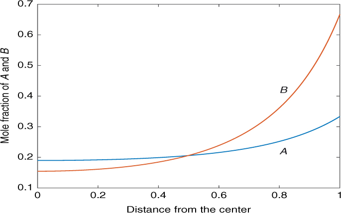
Figure 15.1 Composition profiles of the example studied in this section. The parameters align with those in Listing 15.1.
It is fairly easy to modify and apply this code for multiple reactions. The rate of reaction can be calculated by using the stoichiometric matrix and a rate function for each reaction. Thus the rate of production for species i is given by the summation of its rate of production from all the reactions (subscript r) as
where nr is the number of reactions, νri is the stoichiometry of the ith species in the rth reaction and is the rate term for the rth reaction (which represents the molar rate of production of any species with unit stoichiometry). The rate term is now introduced into the species balance equations:
Equations 15.4, the constitutive model and Equation 15.8, the conservation model, have to be integrated together now. There are two equations for each species (one for the conservation law and the other for the constitutive model) and hence there are 2 * ns-first order differential equations to be solved simultaneously. These are boundary value types of problems.
Note that the number of equations can be simplified using the rank of the stoichiometric matrix; this is left as an exercise. For example, if there is a single reaction then there is only one independent flux, usually the flux based on a key component. The flux of all other species is determined simply by the stoichiometry of the reaction. Here we keep all 2 * ns equations for simplicity. This takes up slightly more computational time but keeps the implementation to new problems somewhat simpler.
For porous catalysts both Knudsen and bulk diffusion may be important. In such cases the contributions are added together and the Stefan-Maxwell model is modified as
Here DKe,i is the effective Knudsen diffusivity of i while Dij,e is the effective binary pair gas phase difficulty (D corrected with the porosity and tortuosity factors).
The relative magnitude of the two terms in Equation 15.9 determines the nature of the solution method. If Knudsen dominates the fluxes are uncoupled while if the bulk gas diffusion dominates we expect multicomponent coupling effects, especially if the molecular weights of the diffusing species are vastly different. Uncoupled problems can be reduced to a set of second-order differential equations in concentrations and solved directly. Coupled problems are best solved by simultaneous computations of fluxes and concentrations by the code shown in Listing 15.1.
15.3 Heterogeneous Reactions
Illustrations of computations to a heterogeneous reaction are presented in this section. Consider a case where the reaction
A → B + C
is taking place over a catalyst surface.
Then by stoichiometry the following conditions apply for the fluxes:
NB = –NA and NC = –NA
Thus NB and NC can be eliminated from the Stefan-Maxwell equations. In addition the mole fraction of one of the species, say, C, can also be eliminated using
yC = 1 – yA – yB
The Stefan-Maxwell equation for A reduces to the following equation when these conditions are applied:
The equation for B becomes
The condition that no homogeneous reaction takes place provides the third equation:
Thus we track three variables simultaneously: yA, yB, and NA. Three boundary conditions are needed to solve the problem. The gas composition in the bulk gas is specified, which provides two conditions. The additional condition to be imposed is based on the kinetics of the heterogeneous surface taking place at the surface and is discussed in the following.
For fast reactions the Dirichlet condition is applied at the reacting surface. The mole fraction of A at the surface is now set as zero, which provides the third boundary condition. These equations can be used to solve for NA and also for yB,L, the mole fraction of B at the reacting surface.
For a finite reaction case, the balance of flux of A at the reacting surface leads to the following boundary condition at the surface:
NA(z = L) = –RA = ksCyAs
Note that the last term is specific for a first-order reaction at the catalyst surface. (z = L is the location of the reacting surface.) Thus a Robin type of boundary condition is now specified at the reaction surface.
This completes the problem specification; the system equations can be implemented in BVP4C and solved. Example 15.1 provides an illustration.
Example 15.1 Ternary Diffusion with a Heteogeneous Reaction
Vapor phase dehydrogenation of ethanol (designated as A or 1) to produce acetaldehyde (2) and hydrogen (3) was studied by Froment, Bischoff, and de Wilde (2011) and is an example of a system of the preceding type where a heterogeneous catalytic reaction takes place on a surface:
ethanol → acetaldehyde + hydrogen
The kinetics of the heterogeneous reaction was modeled as
Rate = –ksyA with ks equal to 10.0 mol/m2 s mole fraction
The bulk gas phase concentration was y1 = 0.6, y2 = 0.2, and y3 = 0.2. Find the rate of reaction assuming a mass transfer film thickness of 1 mm. Temperature = 548 K and pressure = 101.3 kPa. The binary diffusion coefficients are D12 = 7.2 × 10⁻⁵ m2/s, D13 = 23.0 × 10⁻⁵ m2/s, and D23 = 23.0 × 10⁻⁵ m2/s.
Solution
The Stefan-Maxwell model is written for each of the species, resulting in three differential equations. These are simplified using the determinancy condition and the constraint on the mole fraction to two equations. The resulting equations are linear and hence they can be set up in matrix form so that the solution can be written, in principle, in terms of the expm function. Finally the boundary conditions at the surface are applied to close the problem and the resulting nonlinear algebraic equations are solved by FSOLVE or similar routines. The unknown variables are the mole fractions of species 1 and 2 at the catalytic surface.
An alternative is to integrate the system of equations by using the BVP4C solver in MATLAB. The code prsented in Listing 15.1 can be easily adapted for this case.
The following values of the mole fraction at the catalytic surface should be obtained upon using either of these procedures:
y1 = 0.0592, y2 = 0.6055, and y3 = 0.3353
Note the low value of y1 (compared to bulk) indicates significant mass transport resistance. The flux of A is computed from the code as 0.9473 mol/m2s.
15.4 Non-Reacting Systems
Application to non-reacting systems based on the film theory of mass transfer is discussed in this section. The first example is the multicomponent version of the evaporation of liquid in a container. The binary version was studied in Section 6.2.
15.4.1 Evaporation of a Liquid in a Ternary Mixture
Consider a liquid evaporating into an open space in a tube. The system analyzed in Section 6.2 was a binary mixture; A was the evaporating species while B was the inert gas into which A was evaporating. The use of a determinancy condition led to the following equation for the flux of A:
This, integrated across the system, provided an expression for the flux (Equation 6.18). In this section we extend the model to a ternary system with A evaporating into an inert gas mixture of B and C.
One approach is to use the pseudo-binary diffusivity for A, DA–m, which can be calculated from the Wilke equation shown in Section 5.3. The expression for the flux then has a similar form as that for a binary:
Let us explore this in connection with the Stefan-Maxwell model first, where we show that for this specific problem it is an exact result that can be derived from the Stefan-Maxwell model. However, we will find that a unique value for DA–m cannot be assigned immediately. A value based on some average composition has to be calculated and used.
Here we solve the Stefan-Maxwell model directly without having to use the pseudo-binary approach. First we demonstrate that the Wilke equation results from simplification of the Stefan-Maxwell equation.
Basis for Wilke Equation
The Stefan-Maxwell model transport of species A in a ternary mixture is
If we have UMD then NB and NC are zero, which provides the determinacy condition. These are now used in the above equation, which simplifies to
Rearranging this we have the following expression for the flux:
The combined flux above is the sum of the diffusion and convection flux:
NA = JA + yANt
For the system being studied, Nt = NA. Also, expressing the diffusion in terms of a pseudo-binary diffusivity of A in the mixture, DA–m, we have
Comparing this expression with that defined using the pseudo-binary diffusion coefficient (Equation 5.23 in Chapter 5), we find the pseudo-binary is defined according to the Wilke equation as
This is the basis for the Wilke equation. It therefore applies strictly speaking when only one species (A) is diffusing in a ternary mixture. The other two species have zero fluxes. Note that this is used as an approximation often even when these conditions do not hold. Hence the flux is given as
The advantage of this over the Stefan-Maxwell model is that it is flux explicit and similar to that for a binary case. The disadvantage is that DA–m is mole fraction dependent (as can be seen from Equation 15.19) and hence varies along the diffusion or reaction path and has to be based on some representative mole fraction in the system. We do not know the mole fraction profiles a priori. The mole fractions are known in the bulk gas and can be used to find the pseudo-binary diffusivity as an approximation.
As an alternative we can track the concentration profiles for B and C, in other words solve the Stefan-Maxwell formulation directly. This approach is rather general and explored further in this section.
Evaporation in Ternary: Stefan-Maxwell Model
Let us formulate two differential equations for B and C using the Stefan-Maxwell formulation. We can use these conditions as simplifications:
yA = 1 – yB – yC
Also NB = 0 and NC = 0 (UMD).
With these substitutions the flux expressions for B and C are as follows:
and
Each equation can be integrated separately here since NA is not a function of z. Note that this is not always true, for example, if a simultaneous homogeneous reaction of A is also taking place.
Integration with the boundary condition at z = L (the bulk gas) gives
yB = yBL exp[–N*(1 – z/L)]
and
yC = yCL exp[–N* (1 – z/L)]
where N* is a dimensionless flux defined as
and β is the diffusivity ratio defined as DAB/DAC.
Finally, applying the boundary condition at the surface, z = 0, (where the mole fraction of A is known by equilibrium considerations) we have
which provides an implicit equation for find N*.
We also note that the binary expression is recovered if β = 1, that is, when the binary diffusivity of A in B is the same as that for A in C, DAB = DAC. The effect of multicomponent interaction therefore depends on the β parameter.
15.4.2 Evaporation of a Binary Liquid Mixture
Here we consider a similar problem with now the liquid containing a mixture of two species, A and B. This mixture is evaporating into a inert gas C. The problem is now to compute both NA and NB.
Since C is inert we can set NC = 0, which is the required determinacy condition. Also, since the mole fractions add up to unity, we have yC = 1 – yA – yB.
When these simplifications are introduced into the Stefan-Maxwell equations, we obtain the following equations for the mole fraction profiles of A and B:
and
The boundary conditions needed are as follows: at the evaporating surface, z = 0, the mole fractions are related to the vapor pressure values (assuming an ideal liquid), while at the bulk gas, z = L, the mole fractions are specified from the bulk gas values. Often a value of zero is used as a simplification.
The above differential equations are first order and look like initial value problems (IVPs); they are candidates for explicit marching in z or solvers such as ODE45. However, the fluxes are unknown and have to be computed by imposing the boundary condition at x = L. Hence this is a boundary value problem. We discuss two methods for solution of this problem. First is the direct use of BVP4C, which is similar to that discussed in Section 15.2. The second is based on matrix algebra, which is discussed next.
Matrix Method
Equations 15.22 and 15.23 can be expressed in matrix form as
where y is the solution vector; in the present case the solution vector has a dimension of two, representing yA and yB.
The term à above is the coefficient matrix and R is the non-homogeneous term. Since both the coefficient matrix and non-homogeneous term are constants, the solution can be represented in matrix form using the exponential matrix concept:
y = (y0 + Ö1R)expm(Az) – Ö1R
where y0 is the mole fraction at the evaporating surface.
Now using the conditions at the bulk gas the following algebraic relation is obtained:
This equation contains the unknowns NA and NB, which are buried in the à matrix. The solution of these “implicit” algebraic equations gives the fluxes. This can be accomplished, for instance, by using a nonlinear algebraic solver such as FSOLVE in MATLAB. Example 15.2 provides an illustration for evaporation rate in a binary mixture.
Example 15.2 Evaporation Rate in a Liquid Mixture
The problem analyzed here is an Arnold cell containing a binary mixture of acetone (1) and methanol (2). The mixture is evaporating into an inert gas, say air (3). The pressure and temperature are maintained at 99.4 kPa and 328.5 K respectively. The gas composition at the liquid surface is y1 = 0.319 and y2 = 0.528. The height of the Arnold cell was 0.238 m and composition of both vapor species (1) and (2) at this end was zero. Find the evaporation rate and sketch the mole fraction profiles in the cell. This problem is adapted from Taylor and Krishna (1993). The binary diffusion coefficients are D12 = 8.48 × 10⁻⁶ m2/s, D13 = 13.72 × 10⁻⁶ m2/s, and D23 = 19.91 × 10⁻⁶ m2/s.
Solution
The problem was solved by both the matrix method using the MATLAB FSOLVE function for the solution of the algebric equation and by the boundary value method using the BVP4C solver in MATLAB. The results for both cases agree and are as follows:
N1 = 1.78 × 10⁻³mol/m2.s
N2 = 3.13 × 10⁻³mol/m2.s
The concentration profiles are sketched in Figure 15.2. These profiles are in good agreement with the experimental data shown in Taylor and Krishna as well. Students should verify these results by using the code in Listing 15.1.

15.4.3 Equimolar Counter-Diffusion
This section discuses the use of the equimolar counter-diffusion condition as the determinancy condition to relate the fluxes.
An example of equimolar counter-diffusion is found in the modeling of diffusion in a porous plug separating two regions of different gas compositions. The binary case was examined in Example 5.2 and exercise problem 4 in Chapter 6. The compositions at the two ends are specified and the fluxes of the various species are to computed. The determinacy condition used here is that there is equimolar counter-diffusion.
A second example is in distillation of a ternary mixture. Since distillation is usually under adiabatic conditions, we assume equimolar diffusion. This assumes that the molar heat of vaporization of the three species is nearly equal. Then the total flux across the system is zero in order to maintain the heat balance and the problem reduces to equimolaar counter-diffusion.
The Stefan-Maxwell model is simplified by using the following conditions. The total flux is zero, which provides the determinancy Nt = 0, or
NC = –NA – NB
The second simplification to be used in the Stefan-Maxwell model is that mole fractions have to add up to unity and hence
yC = 1 – yA – yB
The mole fraction yC and flux NC are then eliminated from the Stefan-Maxwell equations for both dyA/dz and dyB/dz. The resulting equations can be solved by the matrix method (followed by FSOLVE) or by the BVP4C routine. Example 15.3 shows an application to the flux calculation in the distillation of ternary mixture.
Example 15.3 Distillation of a Ternary Mixture
Estimate the mass transfer rates during distillation of ethanol (species 1), t-butyl alcohol (species 2), and water (species 3) at a point in the column where the following conditions are specified: bulk vapor composition: y10 = 0.6, y20 = 0.13; interface vapor composition: y1 = 0.5, y2 = 0.14; film thickness = 1 mm; The following values may be used for the three binary pair diffusion coefficients: D12 = 8.0 × 10⁻⁶ m2/s D13 = 21.0 × 10⁻⁶ m2/s, and D23 = 17.0 × 10⁻⁶ m2/s.
Solution
The number of species is three and hence six differential equations can be set up, three from conservation law and three from constitutive equations. The mole fractions are specified at both ends and therefore we have six conditions. The problem specification is complete and the BVP4C code (Listing 15.1) can be modified and used. The following values were obtained for the fluxes:
N1 = 8.09 × 10⁻²mol/m2.s
N2 = 0.434 × 10⁻²mol/m2.s
N3 = –8.52 × 10⁻²mol/m2.s
It may be noted that the number of equations to be solved can be reduced to four by using the sum of the mole fraction requirement and the determinacy condition. Computations are not intense even with six equations and hence this simplification is optional.
Some interesting results pertinent to diffusional interaction effects are now available. Note that component 2 diffuses against its concentration gradient, an example of reverse diffusion. The mole fraction is 0.13 on one side and 0.14 on the other side, as specified in the problem, but the flux is positive!
The conditions simulated leading to reverse diffusion are shown in Figure 15.3 for t-butyl alcohol (species 2). Species 2 moves from left to right while Fick’s law would indicate it should move the other way.

Figure 15.3 Illustration of reverse and osmotic diffusion for t-butyl alcohol (species 2) for the conditions studied in Example 15.3.
We now change the problem specification slightly to indicate the phenomena of osmotic diffusion (Case 2). We set y2 = 0.13, adjusting the mole fraction of C. The following values can now be computed and students should verify these by running the code:
N1 = 8.30 × 10⁻²mol/m2.s
N2 = 0.79 × 10⁻²mol/m2.s
N3 = –9.10 × 10⁻²mol/m2.s
Species 2 diffuses to the liquid even though its own mole fraction is the same both in the vapor and the interface, which is an example of “osmotic” diffusion. The effect is due to the multicomponent diffusion coupling of the transport of three species.
The conditions simulated to leading to osmotic diffusion are also shown in Figure 15.3. Species 2 moves from left to right while Fick’s law would indicate it should have no flux.
The major flux components are due to ethanol (1) and water (3) and these are in opposite directions. These are much larger (in magnitude) than the t-butyl alcohol flux. The flux of t-butyl alcohol varies to satisfy the equimolar constraints and therefore shows unusual effects.
15.5 Multicomponent Diffusivity Matrix
In this section we discuss an inverted formulation of the Stefan-Maxwell model that has been used in many earlier studies (e.g., Toor, 1957; Stewart and Prober, 1964). Although the direct numerical solution of the Stefan-Maxwell model is efficient these days due to many computational tools, the inverted form has many useful pedagogical values and is also useful if one wishes to follow some of the earlier literature in this field.
An inverted formulation of the Stefan-Maxwell model leads to a generalized Fick’s law for diffusion fluxes. The form of the equation is similar to a binary mixture and is the vector analog of the law. A matrix is introduced for the diffusivities in this model.
We consider a ternary system for simplicity. Extension to quaternary systems and so on is straightforward but lengthy.
The idea is to write the diffusion flux explicitly. Since the diffusion flux of species A (denoted as 1 here) may depend on the mole fraction gradient of both A (1) and B (2), it is written as
Here is used as the coefficient matrix and is a measure of the diffusion coefficients. Note that these are not binary pair diffusion coefficients and the relation between the two will be shown soon. Hence the symbol is used for this matrix. Note that ∇y3 is not independent and therefore not used in the flux expression.
A similar equation is written for species 2:
Thus we use four constants to model the diffusion. These four constants can be put into a matrix, which is called the generalized Fick’s law diffusion matrix. Also note that the equation for species 3 is redundant since the diffusion fluxes have to add up to zero.
Note: Although four values for are needed for a ternary case (and (ns – 1)2 in general for a ns component system), there are some restraints between these values, which reduces it to three independent values or ns(ns – 1)/2 in general. These are shown by De Groot and Mazur (1968). The restraint arises from what are known as Onsager reciprocal relations. But in practice these restraints are difficult or even impossible in most cases to apply and the four for binary or (ns – 1)2 values in general are commonly used.
15.5.1 Matrix Relation to Binary Pair Diffusivity
The expression for the matrix can be evaluated by matrix inversion of the Stefan-Maxwell model and the procedure follows.
The Stefan-Maxwell model in diffusion flux form (Equation 15.5) is used here, and is repeated for ease of reading:
A similar equation holds for species 2. We take ns = 3 here, that is, a ternary system.
Two substitutions are made here: (1) J3 = –(J1 + J2) since the diffusion fluxes have to add up to zero and (2) y3 = 1 – (y1 + y2), as the summation of mole fractions should be one.
This permits the flux and the mole fraction of the species to be eliminated from the Stefan-Maxwell equation. The eliminated species is sometimes called the solvent. The resulting equation after some simple algebra is
where ns represents the species that was eliminated, species 3 for the ternary case considered above. The summation is not applied if i equals j.
Equation 15.26 can be represented in compact vector-matrix form as
Here is a 2 by 2 coefficient matrix for a ternary system. This matrix is obtained by gathering all the coefficients of Ji on the right-hand side of Equation 15.26.
The matrix representation can be inverted to obtain J in terms of the mole fraction gradients and the resulting equation can be represented as
where is equal to
Equation 15.28 defines the diffusivity matrix and has a form similar to Fick’s law except that it is now in a vector matrix form. The matrix is the tensor equivalent to the binary diffusivity. The form above is often referred to as the generalized Fick’s law.
The explicit form for the matrix can be obtained for a ternary system analytically and are presented in Table 15.1.
Table 15.1 Explicit Expressions for the Matrix for a Ternary System
An often quoted and well studied problem is the hydrogen(1)-methane(2)-argon(3) system and we calculate the values of for this case from the equation shown previously for a composition of y1 = 0.2, y2 = 0.2, and y3 = 0.6; the results are as follows:
Note the reasonably large value for the cross-diagonal term 21. Complex diffusion effects are signaled by this term. Also note that the coefficients are concentration dependent, unlike the binary pair values. We have calculated this for one composition but if you do this for another composition you will get a different set of values. The diffusivity matrix based on an average composition along the diffusion path is often used as the representative values and the composition dependency is ignored as an approximation.
Another point to note is the choice of the third component, that is, the species that is eliminated in the Stefan-Maxwell model. In the above case argon was eliminated and equations for the diffusion fluxes of the other two species are obtained from the diffusivity matrix. The coefficients will be different if another species, say hydrogen, is eliminated.
Multicomponent diffusion in liquids is often modeled by this approach and the matrix is fitted to experimental data. This is therefore more of an empirical approach. Often the non-ideal effects are not considered explicitly and lumped into the matrix. Similarly, diffusion in ternary solid alloys are often fitted in this manner.
The advantage of diffusion matrix formulation is that the models are analogous to a matrix version of Fick’s law. Hence linear algebra–based methods can be used to get a quick analytical solution. However the matrix is mole fraction dependent. Hence it has to be evaluated at some average mole fraction in the domain and further a constant value for this matrix has to be assigned. Such a model is called the linearized model, first introduced in the field by Toor (1957). On the other hand, in the direct solution method no such assumption is needed, but the problem has to be solved by numerial methods as shown in Section 15.2.
Summary
Stefan-Maxwell equations provide a convenient constitutive model for multicomponent systems. The model is shown to be accurate for ideal gases at low pressures. The model equation is given by Equation 15.4 and is worth memorizing. The values of only binary pair diffusion coefficients, one for each pair in the mixture, are needed. Thus for a ternary mixture we need three diffusion coefficients: D12, D21, and D23.
Stefan-Maxwell equations need to be supplemented with the species conservation laws and some determinancy condition relating the fluxes of various species, similar to that done for a binary mixture. Common conditions useful in many problems are only one non-diffusing gas (uni-molecule diffusion or UMD), equimolar counter-diffusion (EMD) and reacting systems where the fluxes are related by reaction stoichiometry.
The main difficulty in computations with the Stefan-Maxwell model is that the equations are implicit in fluxes. We often wish to compute the fluxes given the mole fraction gradients but Stefan-Maxwell gives the mole fraction gradients in terms of all the component fluxes.
One solution method, applicable when there are no homogeneous reactions, is the matrix method. A matrix-vector solution can be written formally in terms of the exponential matrix. The fluxes are implicit in the coefficients of this exponential matrix and can be solved by a nonlinear algebraic equation solver. Once the fluxes are computed the mole fraction profiles can be calculated using the formal matrix-vector solution.
A second method is to augment the Stefan-Maxwell equations with species mass balance equations. The resulting problem is of a boundary value type and can be solved using any standard package for the solution of boundary value problems, for example BVP4C. Code based on this is provided in Listing 15.1.
An inverted formulation of Stefan-Maxwell models leads to a generalized Fick’s law for diffusion fluxes. The form of the equation is similar to a binary mixture and is the vector analog of the law. The matrix appearing in this expression, the matrix, can be calculated from the binary pair values at an average concentration in the system. Once this matrix is evaluated, solution methods for binary systems have a direct vector-matrix analog that may be useful for solution of many problems.
The matrix is concentration dependent. An often used simplifying assumption is that the concentration dependency of is ignored. This is often referred to as a linear model for multicomponent diffusion. Linear algebra tools can then be used to solve the model equations.
Complexities associated with multicomponent diffusion can be associated with the off-diagonal terms of the matrix. If these terms are small or zero then each species diffuses in proportion to its own gradient. Complexities such as reverse diffusion, osmotic diffusion, and so on, are absent in such cases.
The matrix can also be viewed as a fitted parameter relating the fluxes to the mole fraction gradients and used as such in an empirical setting. Such an approach for instance is useful for non-ideal systems.
Review Questions
15.1 What is the molecular basis for the Stefan-Maxwell model?
15.2 What is the basis for the Wilke equation for the pseudo-binary diffusion coefficient?
15.3 Under what conditions is the Wilke equation an exact representation of the Stefan-Maxwell model?
15.4 When is the exponential matrix-based method not suitable for solution of multicomponent diffusion problems?
15.5 What are reverse diffusion and osmotic diffusion?
15.6 If two independent reactions take place and there are five species, how many of the species fluxes are independent?
15.7 Define a diffusivity matrix and distinguish its components from binary pair diffusion coefficients.
15.8 What is the difference between D12 and 12?
15.9 Can D11 be non-zero? Can 11 be non-zero?
15.10 What is the implication of 12? Can it be zero?
Problems
15.1 Evaporation into a mixture of two inert gases. Acetone is evaporating in a mixture of nitrogen and helium. Find the rate of evaporation and compare it to the rate in pure nitrogen and pure helium.
15.2 Comparison of Stefan-Maxwell model with Wilke model for ternary evaporation. Compare the results in exercise problem 1 with the model using a pseudo-binary diffusivity value for acetone. The pseudo-binary diffusivity can be calculated from the correlation given by Wilke.
15.3 Evaporation of a binary mixture: expm-based code. Write MATLAB code to solve Equations 15.22 and 23 for the unknowns NA and NB. You will need to write a function m-file to be used in FSOLVE, which takes in trial values of NA and NB, calculates the A and R matrices based on these values, and returns two equations based on Equations 15.22 and 15.23 as the function values. FSOLVE will then iterate using this function program to find NA and NB.
Test the results for the data given in Example 15.2.
15.4 Arnold cell analysis for a binary liquid. A binary mixture of A and B is contained in a tube with a starting level of H0. Over time evaporation proceeds and the level changes with time. Develop a model to calculate the level change in the tube. Note that the mass balances for A and B in the liquid are needed since they change in different manners with time. Thus the liquid will get enriched with the less volatile compound.
15.5 CO diffusion to a catalytic surface followed by a heterogeneous reaction. Catalytic oxidation of CO is an important reaction in pollution prevention. The reaction scheme is
O2(A) + 2CO(B) → 2CO2(C)
Set up the Stefan-Maxwell model for this problem. State the determinacy condition and simplify the equations into two differential equations for the mole fractions of any two of these species. Calculate the solution for the mole fraction profiles and find the values of the fluxes using the matrix method and the BVP method. Assume fast reaction at the catalyst surface.
15.6 Rank of a stoichiometric matrix to find the invariant relations between the component fluxes. Examine how the rank of the stoichiometric matrix can be used to reduce the number of equations to be solved. For example, if there are ns components and nr equations we can show that only ns – nr independent mass balance equations are needed. The remaining variables form an invariant that connects the flux of the selected key components to those of the non-key components. Write MATLAB code to find the invariant given a stoichiometric matrix.
15.7 Methane reforming in a porous catalyst. Extend the analysis in Section 15.2 to two reactions that are applicable for steam reforming of methane. The first reaction is
CH4 + H2O CO + 3H2
followed by the water-gas shift reaction. Kinetic and diffusion parameters can be found in the work by Haynes (1984) or other sources.
15.8 matrix values for hydrogen-methane-argon mixture. Consider the calculation of a generalized diffusion coefficient (
These values are for a composition of x1 = 0.2 and x2 = 0.2. The units are cm2/s. Argon was used as the species that was eliminated from the Stefan-Maxwell equation.
Verify the results if the binary pair values are D12 = 0.726; D13 = 0.902 and D23 = 0.218 at 307 K temperature. Units are cm2/s.
15.9 Effect of composition numbering on the Fick matrix . In the matrix calculation of , a particular species n chosen for elimination is usually referred to as the solvent. For example, in the above example argon was chosen as the reference. The choice of “solvent” species is arbitrary but it can have an effect on the coefficient and the structure of the resulting matrix. For this exercise use argon (1), methane (2), and hydrogen (3). Eliminate hydrogen rather than argon, which was done in the previous exercise. Use the same composition as earlier. Show that the matrix is now
15.10 Transient profiles in a two bulb apparatus. Derive the solutions for transient concentration profiles in the two bulb apparatus (Example 6.4 in the text) for a binary case and show that the multicomponent case can be derived as an extension of this. What assumption is implicit in extending the binary case to the multicomponent case?