
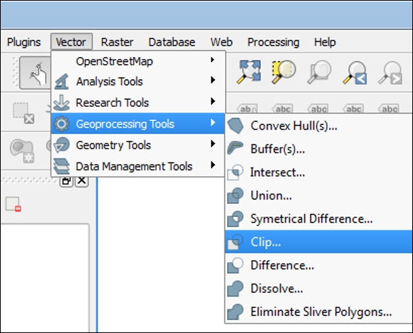
This section will focus on geoprocessing tools that use vector data layers as inputs to produce derived outputs. The geoprocessing tools are part of the fTools plugin, which is automatically installed with QGIS and enabled by default. The tools can be found in the Geoprocessing Tools menu under Vector. The icons next to each tool in the menu give a good indication of what each tool does.
We will look at some commonly used spatial overlay tools such as clip, buffer, and dissolve. In the case of a simple analysis, these tools may serve to gather all the information that you need. In more complex scenarios, they may be part of a larger workflow:
Note
The tools covered in this chapter are also available via the Processing Toolbox, which is installed by default with QGIS Desktop. When enabled, this plugin turns on the Processing menu from which you can open the Processing Toolbox. The toolbox is a panel that docks to the right side of QGIS Desktop. The tools are organized in a hierarchical fashion. The toolbox contains tools from different software components of QGIS such as GRASS, the Orfeo toolbox, SAGA, and GDAL/OGR, as well as the core QGIS tools covered in this chapter. Some tools are duplicated. For example, the GRASS commands, SAGA tools, and QGIS geoalgorithms all include a buffer tool. With the default installation of QGIS 2.14, the toolbox contains almost 500 tools; so, the search box is a convenient way to locate tools within the toolbox. For a more detailed look at the Processing Toolbox, refer to Chapter 8, The Processing Toolbox.
The screenshot following shows the Processing Toolbox with the Search box at the top:

Spatially overlaying two data layers is one of the most fundamental types of GIS analysis. It allows you to answer spatial questions and produce information from data. For instance, how many fire stations are located in Portland, Oregon? What is the area covered by parks in a neighborhood?
This series of spatial overlay tools compute the geometric intersection of two or more vector layers to produce different outputs. Some tools identify overlaps between layers and others identify areas of no overlap. The spatial overlay tools include Clip, Difference, Intersect, Symmetrical Difference, and Union.
These two tools are related in that they are the inverse of each other. Data often extends beyond the bounds of your study area. In this situation, you can use the Clip tool to limit the data to the extent of your study area. It is often described as a cookie cutter. It takes an input vector layer and uses a second layer as the clip layer to produce a new dataset that is clipped to the extent of the clip layer. The Difference tool takes the same inputs, but outputs the input features that do not intersect with the clip layer.
In this example, we will clip fire stations to the boundary of the city of Portland. Load the fire_sta.shp and PDX_city_limits.shp files from the sample data. Select fire_sta in the Input vector layer field and PDX_city_limits in the Clip layer field. The output shapefile will be loaded into QGIS automatically since Add result to canvas is checked. This is the default setting for most tools. If you have any selected features, you can choose to just use them as inputs. The operation creates a fire stations layer consisting of the 31 features that lie within the Portland city limits:

Using the Difference tool with the same inputs that were used with Clip results in the output fire stations that lie beyond the limits of the clip layer. The outputs from these two tools contain only attributes from the Input vector layer:
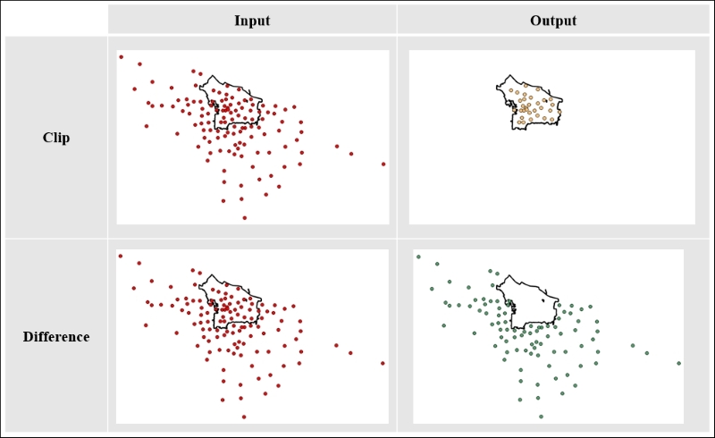
Inputs and outputs from the Clip and Difference tools
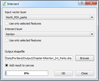
The Intersect tool preserves only the areas common to both datasets in the output. Symmetrical Difference is the opposite; only the areas that do not intersect are preserved in the output. Unlike Clip and Difference, the output from these two tools contains attributes from both input layers. The output will have the geometry type of the minimum geometry of the inputs. For example, if a line and polygon layer are intersected, the output will be a line layer. The following is an example of running the Intersect tool. After that, you will see a screenshot that demonstrates the output from each tool.
The following examples use the North_PDX_parks.shp and Kenton.shp shapefiles from the sample data:
The following screenshot compares the Intersect and Symmetrical Difference tools by showing example inputs and outputs for each:

The Union tool overlays two polygon layers and preserves all the features of both datasets, whether or not they intersect. The following screenshot displays an example union using the North_PDX_parks.shp and Kenton.shp shapefiles from the sample data. Attributes from both datasets are contained in the output attribute table:
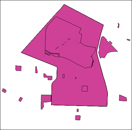
Output of the Union tool
The Buffer tool is a commonly used tool that produces a new vector polygon layer which represents a specific distance from the input features. It can be used to identify proximity to a feature. Here, we will buffer the Portland fire departments by one mile; this will identify all the areas within the one-mile buffer distance. To buffer, we will perform the following steps:
- The Input vector layer field will be set to
Portland_FireStations. - Next, we'll specify the buffer distance. The tool will use the units of the coordinate reference system of the input vector layer as the distance units. This data is in State Plane Oregon North with the unit as feet. Enter
5280to produce a one-mile buffer. You also have the option of specifying an attribute column containing buffer distances. This allows you to specify different buffer distances for different features. - QGIS cannot create true curves, but it provides an option to set Segments to approximate. The higher the number, the smoother the output will be because QGIS will use more segments to approximate the curve. In this example, it has been set to
20instead of the default of5: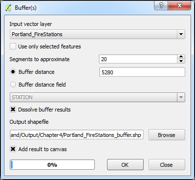
- Checking Dissolve buffer results will merge buffer polygons if they overlap:
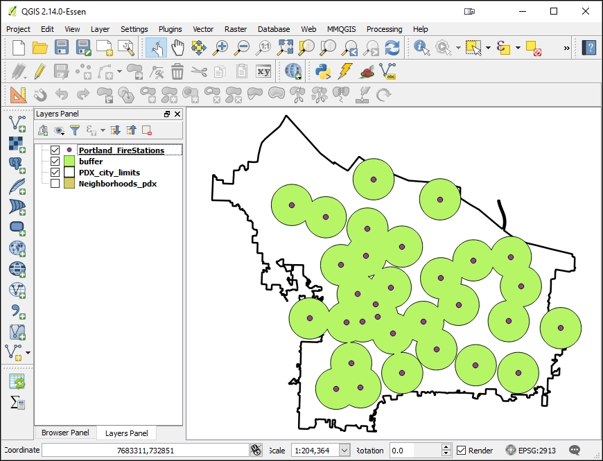
- The output is a polygon dataset representing the specified distance from the input features.
The Convex Hull tool will take a vector layer (point, line, or polygon) and generate the smallest possible convex bounding polygon around the features. It will generate a single minimum convex hull around the features or allow you to specify an attribute column as input. In the latter case, it will generate convex hulls around features with the same attribute value in the specified field.
The result will be the bounding area for a set of points, and it will work well if there are no outlying data points. Here, a convex hull has been generated around Portland_FireStations.shp:

The Dissolve tool merges the features of a GIS layer. It will merge all the features in a layer into one feature. This can be done via the values of an attribute field or with the Dissolve all option. In the following example, the neighborhoods of Portland (Neighborhoods_pdx.shp) are dissolved, which creates the city boundary:
