
Maps and aerial photographs in hard copy have a lot of valuable data on them. When this data needs to be brought into a GIS, they are digitally scanned to produce raster imagery. The output of a digital scanner has a coordinate system, but it is a local coordinate system created by the scanning process. The scanned imagery needs to be georeferenced to a real-world coordinate system before it can be used in a GIS.
Georeferencing is the process of transforming the coordinate reference system (CRS) of a raster dataset into a new coordinate reference system. Often, the process transforms the CRS of a spatial dataset from a local coordinate system to a real-world coordinate system. Regardless of the coordinate systems involved, we'll call the coordinate system of the raster to be georeferenced the source CRS and the coordinate system of the output the destination CRS. The transformation may involve shifting, rotating, skewing, or scaling the input raster from source coordinates to destination coordinates. Once a data set has been georeferenced, it can be brought into a GIS and aligned with other layers.
Georeferencing is done by identifying ground control points (GCP). These are locations on the input raster where the destination coordinate system is known. Ground control points can be identified in one of the following two ways:
- Using another dataset covering the same spatial extent that is in the destination coordinate system. This can be either a vector or a raster dataset. In this case, GCPs will be locations that can be identified on both the datasets.
- Using datums or other locations with either printed coordinates or coordinates that can be looked up. In this case, the locations are identified and the target coordinates are entered.
Once a set of ground control points has been created, a transformation equation is developed and used to transform the raster from the source CRS to the destination CRS.
Ideally, GCPs are well distributed across the input raster. You should strive to create GCPs near the four corners of the image, plus several located in the middle of the image. This isn't always possible, but it will result in a better transformation.
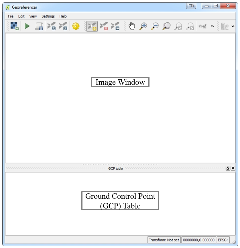
The Georeferencer GDAL plugin is a core QGIS plugin, meaning it will be installed by default. It is an implementation of the GDAL_Translate command-line utility. To enable it, navigate to Plugins | Manage and Install Plugins and then click on the Installed tab and check the box to the left of Georeferencer GDAL plugin. Once enabled, you can launch the plugin by clicking on Georeferencer under Raster. The Georeferencer window has two main windows: the Image Window and the Ground Control Point (GCP) Table window. These windows are shown in the following screenshot:
The general procedure for georeferencing an image is as follows:
-
Load the image to be georeferenced into the Georeferencer image window by clicking on Open Raster under File, or by using the Open raster button (
 ).
).
- If you are georeferencing the raster against another dataset, load the second dataset into the main QGIS Desktop map canvas.
-
Begin to enter ground control points with the Add point tool (This tool,
 , is also available via Edit | Add point). Regardless of which of the two ground control point scenarios you are working with, you need to click on the GCP point within the Georeferencer image window. Use the zoom and pan tools so that you can precisely click on the intended GCP location.
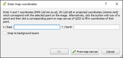
- Once you click on the input raster with the Add point tool, the Enter map coordinates dialog box will open:
You are now halfway done entering the GCP. Follow the appropriate directions provided next. These will be different workflow depending on whether you are georeferencing against a second loaded dataset or against benchmarks, datums, or other printed coordinates on the input raster.
If you are georeferencing against a second loaded dataset, you need to follow these steps:
- Click on the From map canvas button.
- Locate the same GCP spatial location on the data loaded in the main QGIS Desktop map canvas. Click on that GCP location.
- Use the zoom and pan tools so that you can precisely click on the intended GCP location.
- If you need to zoom in to the dataset within the QGIS Desktop map canvas, you will have to first zoom in and then click on the From map canvas button again to regain the Add point cursor and enter the GCP.
- The Enter map coordinates dialog box will reappear with the X / East and Y / North coordinates entered for the point where you clicked on the QGIS Desktop map canvas:

- Click on OK.
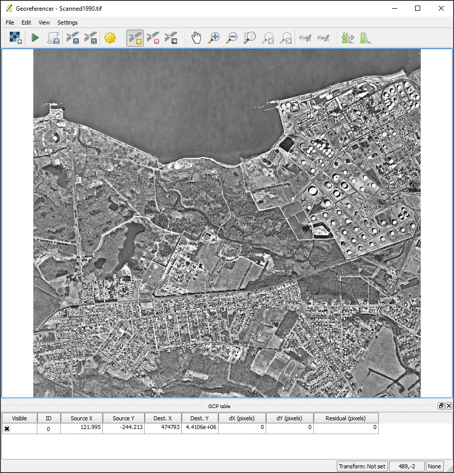
- As you enter GCP information for the source (Source X/Source Y) and destination (Dst. X/Dst. Y) coordinates, they will be displayed in the GCP table window in the Georeferencer window:
- Repeat steps 1-4 and 1-7 to enter the remaining GCPs.
If you are georeferencing against benchmarks, datums, or other printed coordinates on the input raster, you need to perform the following steps:
- Enter the X / East and Y / North coordinates in the appropriate boxes.
- Click on OK.
- Repeat steps 1-4 and 1-2 to enter the remaining GCPs.
Now that you've learned the basic procedure for georeferencing in QGIS, we will go through two examples in greater detail. Here, you will learn all the options for using the Georeferencer GDAL plugin.
In this example, the scanned1990.tif aerial photograph will be georeferenced by choosing ground control points from a more recent aerial photograph of the bridgeport_nj.sid area. The scanned1990.tif image is the result of scanning a hard copy of an aerial photograph. The bridgeport_nj.sid image file covers the same portion of the planet and is in the EPSG:26918 - NAD83/UTM zone 18N CRS. Once the georeferencing operation is completed, a new copy of the scanned1990.tif image will be created in the EPSG:26918 - NAD83 / UTM zone 18N CRS.
- Launch QGIS Desktop and load the
bridgeport_nj.sidfile into the QGIS Desktop map canvas. (Note that you may need to navigate to Properties | Style for this layer and set the Load min/max values option to Min / max so that the image renders properly.) - Click on Georeferencer under Raster to launch the plugin. The Georeferencer window will open.
-
Load the
scanned1990.tifaerial photograph into the Georeferencer image window by clicking on Open Raster under File or by using the open raster button, .
.
- Arrange your desktop so that QGIS Desktop and the Georeferencer window are visible simultaneously.
- Familiarize yourself with both datasets and look for potential GCPs. Look for precise locations such as piers, corners of roof tops, and street intersections.
-
Zoom in to the area, using the zoom-in button (
 ), where you will enter the first GCP in both the QGIS Desktop and Georeferencer windows. Zooming in will allow you to be more precise.
-
Enter the first GCP into the Georeferencer image window using the Add Point tool (
 ).
).
-
After clicking on the image in the Georeferencer image window, the Enter map coordinates window will open. Click on the
 From map canvas button. The entire Georeferencer window will momentarily disappear.
- Click on the same location in QGIS Desktop.
- The Enter map coordinates window will reappear with the destination coordinates, populating the X / East and Y / North boxes. Click on OK to complete the Ground Control Point.
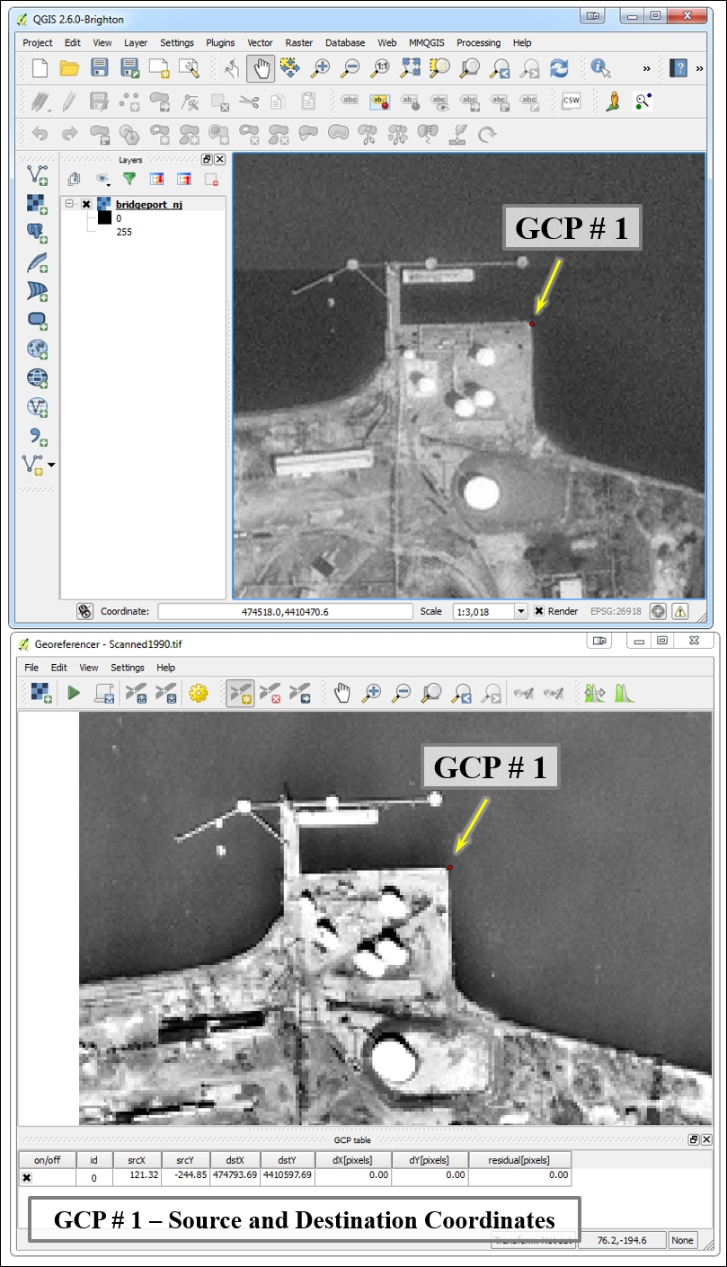
- The GCP table in the Georeferencer window will now be populated with the source and destination coordinates for the first ground control point. The control point will also be indicated in both the Georeferencer image window and QGIS Desktop by a red dot.
Tip
If a GCP has not been precisely placed, the Move GCP Point tool (
 ) can be used to adjust the position of the control point in either the Georeferencer image window or the QGIS Desktop map canvas.
GCPs can be deleted in two ways, as follows:
-
Using the Delete point tool (
 ) and clicking on the point in the Georeferencer image window
- By right-clicking on the point in the GCP table and choosing Remove
-
Using the Delete point tool (
- The following figure shows QGIS Desktop and the Georeferencer window with a single GCP entered:
- Repeat steps 6 to 11 for the remaining ground control points until you have entered eight GCPs.
- Use the pan and zoom controls to navigate around each image, as needed:

-
Once all the points have been entered, the Save GCP Points As button (
 ) can be used to save the points to a text file with a
 .pointsextension. These can serve as part of the documentation of the georeferencing operation and can be reloaded with the Load GCP Points tool ( ) to redo the operation at a later date.
The following steps describe how to set the Transformation settings.
-
Once all the eight GCPs have been created, click on the Transformation settings button (
 ).
).
- Here, you can choose appropriate values for the Transformation type, Resampling method fields, and other output settings. There are seven choices for Transformation type. This setting will determine how the ground control points are used to transform the image from source to destination coordinate space. Each will produce different results and these are described as follows; for this example, choose Polynomial 2:
- Linear: This algorithm simply creates a world file for the raster and does not actually transform the raster. Therefore, this option is not sufficient for dealing with scanned images. It can be used on images that are already in a projected coordinate reference system but are lacking a world file. It requires a minimum of two GCPs.
- Helmert: This performs a simple scaling and rotational transformation. This option is only suitable if the transformation simply involves a change from one projected CRS to another. It requires a minimum of two GCPs.
- Polynomial 1, Polynomial 2, Polynomial 3: These are perhaps the most widely used transformation types. They are also commonly referred to as first (affine), second, and third order transformations. The higher the transformation order the more complex the distortion that can be corrected and the more computer power it requires. Polynomial 1 requires a minimum of three GCPs. It is suitable for situations where the input raster needs to be stretched, scaled, and rotated. Polynomial 2 or Polynomial 3 should be used if the input raster needs to be bent or curved. Polynomial 2 requires six GCPs and Polynomial 3 requires 10 GCPs.
- Thin Plate Spline: This transforms the raster in a way that allows for local deformations in the data. This may give similar results as a higher-order polynomial transformation and is also suitable for scanned imagery. It requires only one GCP.
- Projective: This is useful for oblique imagery and some scanned maps. A minimum of four GCPs should be used. This is often a good choice when Georeferencing satellite imagery such as Landsat and DigitalGlobe.
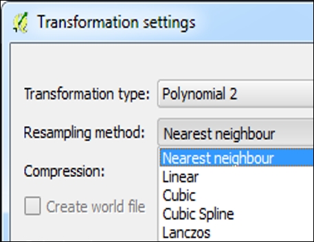
- The following screenshot shows setting the Transformation type setting within the Transformation settings window:

- There are five choices for Resampling method. During the transformation, a new output raster will be generated. This setting will determine how the pixel values will be calculated in the output raster. Each is described here; for this example, choose Linear:
- Nearest neighbour: In this method, the value of an output pixel values will be determined by the value of the nearest cell in the input. This is the fastest method and it will not change pixel values during the transformation. It is recommended for categorical or integer data. If it is used with continuous data, it produces blocky output.
- Linear: This method uses the four nearest input cell values to determine the value of the output cell. The new cell value is a weighted average of the four input cell values. It produces smooth output because high and low input cell values may be eliminated in the output. It is recommended for continuous datasets. It should not be used on categorical data because the input categories may not be maintained in the output.
- Cubic: This is similar to Linear, but it uses the 16 nearest input cells to determine the output cell value. It is better at preserving edges, and the output is sharper than the linear resampling. It is often used with aerial photography or satellite imagery and is also recommended for continuous data. This should not be used for categorical data for the same reasons that were given for the linear resampling.
- Cubic Spline: This algorithm is based on a spline function and produces smooth output.
- Lanczos: This algorithm produces sharp output. It must be used with caution because it can result in output values that are both lower and higher than those in the input.
- The following figure shows setting the Resampling method setting within the Transformation settings window:
- The following tip discusses choosing the Transformation type:
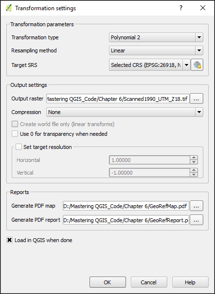
- Choose the target SRS by clicking on the Browse button. A window for choosing the target coordinate reference system will open. For this example, choose EPSG: 26918.
- Name the Output raster by clicking on the Browse button.
- Since raster data tends to be large, it may be desirable to choose a compression algorithm. There are four choices for Compression. Some choices offer better reductions in file size while others offer better data access rates. For this example, use None. The choices are as follows:
- None: This offers no compression
- LZW: This offers the best compromise between data access times and file size reduction
- Packbits: This offers the best data access times but the worst file size reduction
- Deflate: This offers the best file size reduction
- If an output map and output report are desired in the PDF format, click on the browse button next to the Generate pdf map and Generate pdf report options and specify the output name for each. The report includes a summary of the transformation setting, GCPs used, and the root mean square error for the transformation.
- Click on the Set Target Resolution box to activate the Horizontal and Vertical options for output pixel resolution in map units. For this example, leave this option unchecked.
- The Use 0 for transparency when needed option can be activated if pixels with the value of
0should be transparent in the output. For this example, leave this option unchecked. - Click on Load in QGIS when done to have the output added to the QGIS Desktop map canvas.
- Click on OK to set the transformation settings:
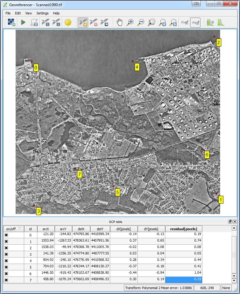
- Once the Transformation settings values have been set, the
residual[pixels]column in the GCP table will be populated. This column contains the root mean square error (RMSE) for each GCP. The mean RMSE for the transformation will be displayed at the bottom of the Georeferencer window.Tip
RMSE is a metric that indicates the quality of the transformation. It will change depending on the Transformation type value chosen. The general rule of thumb is that the RMSE should not be larger than half the pixel size of the raster in map units. However, it is only an indication. Another indication is how well the georeferenced imagery aligns with other datasets.
-
Additionally, the Link Georeferencer to QGIS tool (
 ) and Link QGIS to Georeferencer tool (
 ) will be activated. These will join the Georeferencer window to the QGIS Desktop map canvas, and they will be synced together when you use the pan and zoom tools.
The following screenshot shows the image in the Georeferencer window with eight GCPs entered. Their location is identified by numbered boxes within the image window. The To and From coordinates are displayed in the GCP table window along with the RMSE values:
Click on the Start Georeferencing button (![]() ) button to complete the operation. The georeferenced raster will be written out and added to the QGIS Desktop map canvas if the option was checked in the
Transformation settings window:
) button to complete the operation. The georeferenced raster will be written out and added to the QGIS Desktop map canvas if the option was checked in the
Transformation settings window:

This example will use the zone_map.bmp image. It displays zoning for a small group of parcels in Albuquerque, New Mexico. This image has five geodetic control points that are indicated by small points with labels (for example, I25 28). These control points are maintained by the U.S. National Geodetic Survey (NGS). Here, you will learn how to load a precompiled set of ground control points to georeference the image:
- Load the image into the Georeferencer window.
- Choose EPSG:2903 - NAD83(HARN) / New Mexico Central (ftUS) for the CRS.
-
Click on the Load GCP Points tool (
 ) and choose the
 zone_map.pointsfile. The destination coordinates for the locations in this file were obtained from the NGS website (http://www.ngs.noaa.gov/datasheets/). From the website, theStation Namelink under DATASHEETS was used, and a station name search conducted for each. The destination coordinates are in EPSG:2903 - NAD83(HARN)/New Mexico Central (ftUS). The following figure shows the image in the Georeferencer window with five GCPs entered based on datums whose destination coordinates were looked up online. Their location is identified by numbered boxes within the image window. The To and From coordinates are displayed in the GCP table window along with the RMSE values:
- The
zone_map.pointsfile consists of five columns in a comma-delimited text file. The columns MapX / MapY are the destination coordinates. Columns pixelX / pixelY are the source coordinates, and enable column has a value of1if the GCP is to be used in the transformation and a value of0if it is not to be used. The following are the contents of this points file:mapX,mapY,pixelX,pixelY,enable 1524608.32,1484404.47,7532975.55,-1935414.15,1 1523925.76,1480815.95,6274098.49,-8399918.00,1 1523645.13,1482436.21,5780754.77,-5490891.27,1 1526449.40,1482056.68,10850286.74,-6171365.35,1 1526925.10,1479718.37,11700879.35,-10356281.00,1
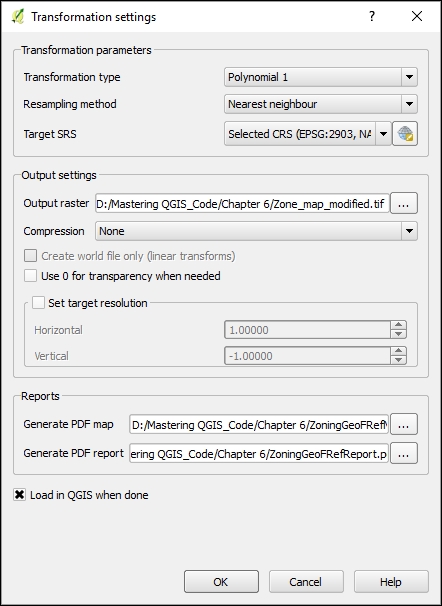
- Click on Transformation settings under Settings and set the following parameters:
- Choose Polynomial 1 as the Transformation type
- Choose Nearest neighbour as the Resampling method
- Choose a Compression of None
- Name the Output raster
- Choose EPSG: 2903 as the Target SRS
- Complete the Generate PDF map and Generate PDF report fields
- Check Load in QGIS when done
- Click on OK
The following figure shows the completed Transformation settings:
-
Click on the Start Georeferencing button (
 ) to complete the operation. The georeferenced raster will be written out and added to the QGIS Desktop map canvas.