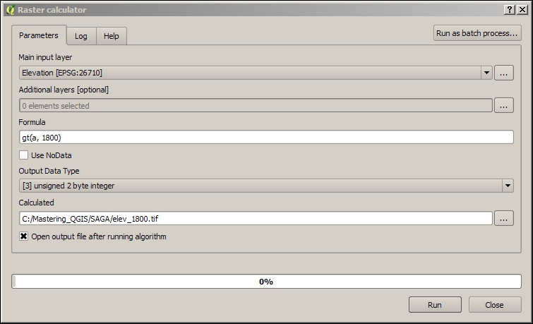
There are multiple ways to create a layer that represents elevation ranges or, in this case, elevation zones that relate to potential habitat. One method would be to use r.recode as we did in the GRASS exercise; another would be to use the Reclassify Grid Values tool provided by SAGA, which we will use later in this exercise; but, another very quick way is to only identify the areas above a certain elevation—in this case, greater than 1,800 meters—using a raster calculator. This type of query will produce a layer with a binary level of measurement, meaning the query is either true or false. To execute the raster calculator, select the layer representing elevation only in the park, enter the formula gt(a, 1800), name the output file, and click on OK.

The syntax we entered in the formula box tells the SAGA algorithm to look at the first grid—in this case a—and if it has a value greater than (gt) 1,800 meters, the new grid value should be one, otherwise it should be zero. The following screenshot illustrates how this appears in the SAGA Raster calculator window. We could have also used the native QGIS Raster calculator tool. So, the intent here is to demonstrate that there are numerous tools at our disposal in QGIS that often perform similar functions. However, the syntax is slightly different between the QGIS, GRASS, and SAGA raster calculators; so, it is important to check the Help tab before executing each of the tools.

After executing this tool, we will be presented with a new raster layer that identifies the elevations above 1,800 meters with a value of 1 and all other values with a value of 0. The next step is to clip the land use layer using the SAGA Clip grid with polygon tool. If you remember, we clipped a raster layer in a previous exercise using the native GDAL Clipper tool, so again this is merely demonstrating the number of options we have to perform spatial operations.

We need to select land use (lulc_clnp) as our input's raster layer, the park boundary as our polygon's layer, name the output file as lulc_clip.tif, and click on OK. Remember from an earlier exercise that you can load the lulc_palette.qml file if you would like to properly symbolize the land use layer, but this step isn't necessary.

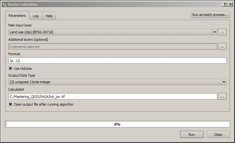
Now, we can query this layer for the areas that represent surface water. We can again use the SAGA Raster calculator tool and enter (a, 11) in the Formula box, as illustrated in the next screenshot. In this example, we are stating that if the land use layer (that is a) is equal to 11, the resulting output value will be 1; otherwise it will be 0.

Now, we have a raster layer that we can use to identify potential habitat within 1,000 meters of surface water.

To accomplish this, we need to create a layer representing proximity to surface water and query that layer for areas within 1,000 meters of any surface water. Our first step is to execute the GDAL Proximity (raster distance) tool in the Processing Toolbox. We need to select the binary (true or false) layer representing surface water (lulc_sw.tif), set the Values field to 1, leave the Distance units field as GEO, change the Output raster type to Int32, leave all the other defaults as they are, and name the output layer as illustrated in the next screenshot:

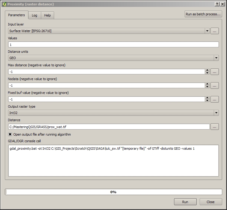
The rationale for setting Values to 1 and Distance units to GEO is that we are asking the algorithm to assume that the distance is measured in increments of 1 based on the geographic distance—in this case, meters—and not on the number of pixels. We can now query the resulting grid for the area that is within 1,000 meters of surface water, but it is important to recognize that we want to identify the areas that are less than 1,000 meters of surface water but greater than 0. If we just query for values less than 1,000 meters, we will produce an output that will suggest that the roosting habitat exists within bodies of water.

The easiest way to perform this query is by using the native QGIS Raster calculator tool by clicking on Raster Calculator under Raster. The following screenshot illustrates how to enter the "Proximity to Water@1" > 0 AND "Proximity to Water@1" <= 1000 syntax to identify a range between 0 and 1,000 meters:

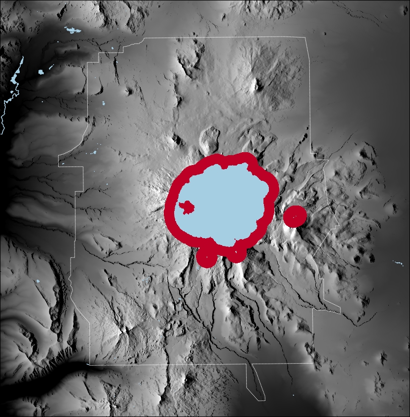
The resulting output will contain the values of 0 and 1, where 1 represents the cells that are within 1,000 meters of surface water and 0 represents those that are beyond 1,000 meters. The next screenshot illustrates what this layer looks like after you set the value of zero to transparent and the buffer itself to red:

The last habitat variable that we need to evaluate is the preference towards roosting in dense forest cover. We are going to reclassify or recode the land use layer assuming that the owls will make use of three primary classes that are deciduous, evergreen, and mixed forest types in decreasing preference. This means that we are going to use a simple ordinal ranking scheme to assign a new value of 3 to grid cells that represent evergreen forest, a value of 2 for shrub cover, a value of 0 for water, and a value of 1 for the remaining land types. We could assume zero for all other cover types, but owls are unpredictable.

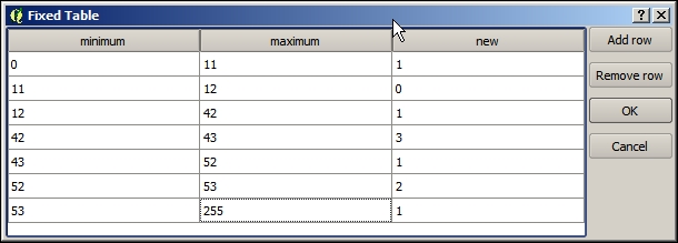
To accomplish this, we could use r.recode as we did in a previous exercise, but instead, we are going to use the SAGA Reclassify Grid Values tool. The advantage of this tool is that we can enter our reclassification rules directly in the tool interface, rather than reading them into the algorithm from a separate file. The following screenshot provides the necessary values to reclassify the land use layer, where 11 represents surface water, 42 represents evergreen forest, 52 represents shrub cover, and all other values are equal to 1. The minimum and maximum columns represent a range of values and within those ranges the resulting pixels will be given the value in the new column:

To use the SAGA Reclassify grid values tool, we need to provide an input grid, which in this case is the clipped land use layer (lulc_clip.tif), and set Method to [2] simple table. The values that need to be reclassified (shown in the previous screenshot) can be entered by clicking on the Fixed table 3x3 button located below the Lookup Table prompt. Make sure you provide a name for the new reclassified grid, for example, lulc_rec.tif.

Now, we have all the necessary layers to finalize our simplistic model of Northern Spotted Owl habitat. Since we have zero values that need to be preserved, that is, places where owls will never roost, we will multiply the three layers together using the SAGA Raster calculator tool. The next screenshot illustrates how to populate the raster calculator by selecting the reclassified elevation layer (elev_1800.tif) as the main input layer and then selecting the reclassified water proximity (buf_water.tif) and land use (lulc_rec.tif) layers by clicking on the ellipsis button (…) next to Additional layers [optional]:

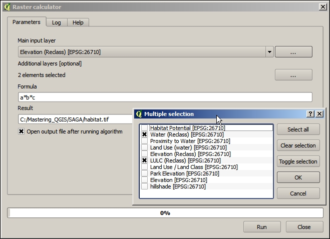
We could have used the native GDAL Raster calculator tool or the GRASS r.mapcalculator tool, but once again, this demonstrates how easy it is to switch between the various toolbox options. Similar to the GRASS syntax, the SAGA algorithm identifies the inputs in the order they are selected as a, b, and c. To ensure that we understand the values reported in the resulting output from this calculation, we need to remember the reclassified water and elevation layers are binary, so it will have the values of 0 and 1, while the reclassified land use layer contains the values from 0 to 3. Therefore, the new layer can only contain values of from 0 to 3 where 0 indicates no habitat, 1 indicates poor habitat potential, 2 indicates moderate habitat potential, and 3 indicates good habitat potential, as illustrated in the next screenshot:

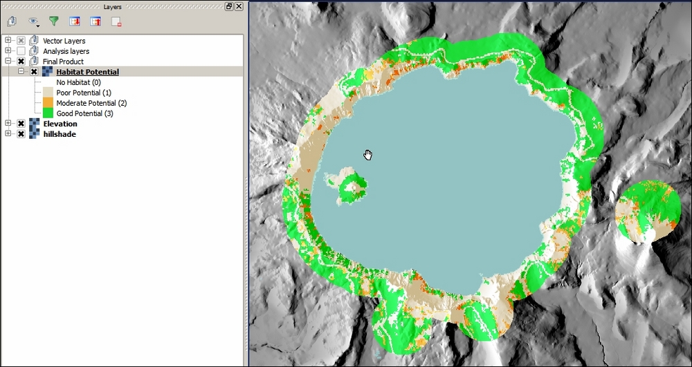
Hopefully, it is clear that this is a very simple model with many assumptions that any ornithologist who actually studies the Northern Spotted Owl would not actually use to evaluate habitat. However, the various tools and general approach that has been taken to evaluate this hypothetical scenario could be applied by paying more rigorous attention to the underlying assumptions about the variables that influence potential habitat. The goals of working through this type of analysis were threefold: to showcase a variety of useful SAGA algorithms, to demonstrate that there are similar tools with subtle differences that are available through the toolbox, and to illustrate how easy it is to switch between native QGIS tools and those found in the toolbox.