
Chapter 5
Implementation and Applications of Microfluidic Quadrupoles
Ayoola T. Brimmo1 and Mohammad A. Qasaimeh1,2
1New York University Abu Dhabi, Division of Engineering, Abu Dhabi, United Arab Emirates
2New York University, Department of Mechanical and Aerospace Engineering, Brooklyn, NY, USA
5.1 Introduction
The quadrupolar configuration (four-pole arrangement) is widely used in several engineering and physical systems and well understood in the electrical, magnetic, acoustic, and gravitational fields. Most famous and practical applications of quadrupoles are the use of quadrupolar magnets to focus beams of charged particles in particle accelerators [1] and the use of quadrupolar electrical fields in mass spectrometers to filter ions based on their mass-to-charge ratio [2]. The main concept behind a quadrupolar configuration is to arrange four identical poles of a field in such a way that a negatively charged pole is always next to a positively charged pole and vice versa. Bringing this analogy to microfluidics, the microfluidic quadrupole (MQ) constitutes four microscale apertures arranged such that an inlet aperture is always located beside an outlet aperture and vice versa [3]. Concurrent charging (injection) and discharging (aspiration) of fluid through this configuration of apertures produces a microfluidic quadrupolar flow pattern, which has streamlines similar to those observed in other quadrupolar fields. Figure 5.1 shows numerically and experimentally obtained flow paths of the typical MQ. Arbitrarily, the two injection apertures are defined as the positive poles, while the aspiration apertures as the negative poles.
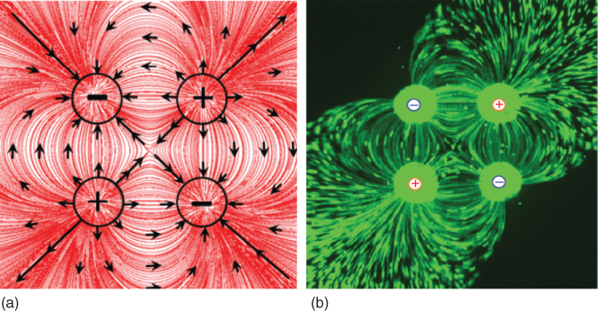
Figure 5.1 Quadrupolar field of microfluidic flows. (a) Numerically calculated flow streamlines of the lateral MQ with identical inlet and outlet flow rates. (b) Experimental image of the flow streaklines of the lateral MQ. Image captured while injecting laced microbeads through the inlet apertures (top right and bottom left) at flow rates identical to the aspiration flow rates through the outlet apertures (top left and bottom right). All aperture diameters are 360 µm.
MQs are typically formed between a four-aperture microfluidic probe (MFP), with pairs of opposing apertures used for injection and aspiration, and a bottom substrate. The MFP can be best described as a channel-less microfluidic device [4] that uses a push–pull configuration for concurrently injecting and aspirating a microfluidic jet from a solution. The device was originally proposed with a flat mesa of two apertures [5], which under Stokes flow conditions can be construed as a microfluidic dipole, with the single injection aperture corresponding to a “+ve” pole and the aspirator to a “−ve” pole [6]. This concept was later extended to the MQ with four apertures, which can also be seen as two dipoles positioned within close proximity. To produce a confined MQ flow pattern, akin to the two-aperture MFP, the ratio of aspiration to injection flow rate for the four-aperture MFP is chosen sufficiently high so that the injected streams are entirely confined.
The MQ can be seen from a fluid dynamics perspective as a planar extensional flow [7]: 2D flow consisting of two opposing inlet streams converging at a junction and exiting through perpendicular outlet channels (see Figure 5.1). This type of flow consists of purely extensional and compressional flow components and a zero fluid velocity point at the junction, called the stagnation point [8]. Characteristically, the flow's velocity magnitude is proportional to the distance from the stagnation point [8], and when all flow rates are identical, the flow is fully symmetrical about the axis connecting the midpoint of similarly charged apertures. In theory, since fluid velocity approaches zero at the stagnation point, diffusion dominates mass transport within this region. Hence, when two different fluids are injected, with a diffusible chemical injected via one aperture – this aperture becomes the chemical gradient source, while the other injection aperture act as the sink – it leads to the formation of a stationary concentration gradient across the region surrounding the stagnation point. The produced gradient is typically stable and controllable and, together with the stagnation point, constitutes the key features of the MQ. The MQs, through these features, have several potential applications in cell biology and life sciences. However, implementation of MQ-based technologies for real-world applications requires a good understanding of how to accurately resolve, and then control, the dynamics of the microscale fluids inherent in its flow structure. These can be achieved by studying the MQ either by analytical formulas, numerical models, or experimental methods. Among these, the experimental approach still represents the benchmark characterization methodology in microfluidics.
In this chapter, we consider the concept behind the MQ, experimental approaches of resolving its flow under steady-state conditions and then look into some of its applications in biology and life sciences. In Section 5.2, we begin our consideration of the MQ by looking into its various forms and highlighting their key features. In Section 5.3, we briefly review the experimental setups and procedures required to experimentally produce MQs. Section 5.4 describes measurements of the MQ's characteristic features, which include regions with stagnation fluid flow, hydrodynamic confinement of injected fluids, and concentration gradient formed within the MQ. In Section 5.5, we review some of the applications of MQ in biology. Finally, Section 5.6 presents our take on the future of MQ and its success factors.
5.2 Principles and Configurations of MQs
As explained in the introduction, quadrupoles are simply a combination of two dipoles positioned within close proximity; thus to generate an MQ, an MFP with four apertures (two inlets and two outlets) have to be arranged such that each inlet aperture (injection) is always next to an outlet (aspiration) aperture and vice versa. In an MQ configuration where all injection and aspiration flow rates are identical, the stagnation point is located at the center of the MQ. Using identical injection and aspiration flow rates, it is very difficult to avoid leakages from the quadrupolar flow into the surrounding medium without using channels. As such, in order to confine the flow, the aspiration flow rate (Qasp) has to be kept reasonably higher than the injection flow rate (Qin); so hydrodynamic flow confinement (HFC) is achieved for both injected fluids. The concept of HFC for the MQ is the same as for the two apertures MFP explained in the previous chapters.
In a typical confined MQ, the size of its stagnation ranges from a point of negligible dimension [3] to a region of about few hundred of micrometers [9], depending on the aperture configuration, flow rates, the gap between the MFP and the bottom substrate, and the fluidic flow threshold considered to be negligible. The stagnation point is typically formed on the midline perpendicular to the axis joining the injection apertures. However, the stagnation point's position, size, and concentration gradient can be manipulated by adjusting the flow rates, and this can be used for hydrodynamically micromanipulating the MQ for dynamic applications.
There are two possible aperture arrangements for the MQ: the lateral and the linear configurations. The lateral MQ is formed under an MFP with four apertures arranged in a classical symmetric quadrupole configuration: alternating charged apertures distributed around the corners of a virtual square (see Figure 5.2a,b). On the other hand, the linear MQ is generated under an MFP with four apertures arranged on a straight line: two inner positively charged apertures (inlets) and two outer negatively charged apertures (outlets) (see Figure 5.2c,d). Key differences between the lateral and linear MQs are the size of their stagnation and the time required to establish steady-state concentration gradients. The stagnation region of the lateral MQ can be mathematically described as a dimensionless point, while that of the linear MQ is postulated to be an area of about a few hundred micometers, depending on the initial design of the MFP, the distance between the two inner injection apertures, and the used injection and aspiration flow rates. As opposed to balancing the inlet and outlet force magnitudes to confine stagnation to a point, as with the lateral MQ, the linear MQ constitutes the balancing of forces to produce a whole region of stagnation. Consequently, the quadrupolar concentration gradient of the lateral MQ is easier and faster to establish and stabilize than that of the linear MQ.
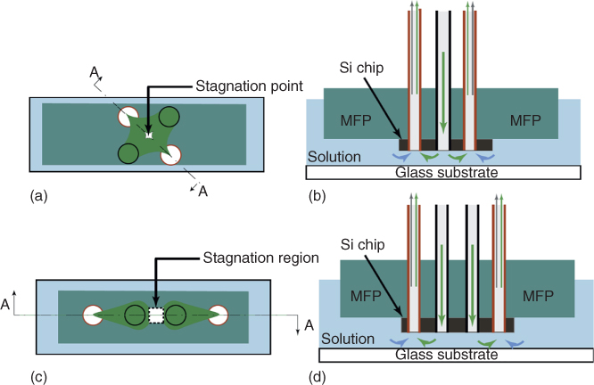
Figure 5.2 2D schematics of the microfluidic probe (MFP) with four apertures arranged for the generation of MQs. (a) Bottom view of the lateral MFP schematics showing the arrangement of the four circular apertures on the corners of a virtual square. (b) Section A–A of (a) showing the microscopic gap between the MFP and the bottom glass substrate. (c) Bottom view of the linear MFP schematics showing the arrangement of the four circular apertures equally distributed along a line. The two inner apertures are used to inject fluids, while the two outer apertures are used for aspirations. (d) Section A–A of (c) showing the microscopic gap between the MFP and the bottom glass substrate. These setups are located on top of an inverted microscope to aid flow visualization.
Simultaneous injection and aspiration of fluids via the apertures of the setups presented in Figure 5.2 generates the quadrupolar flow. In the lateral MQ, the two injected fluids meet head-on at the center and generate the stagnation point with zero flow velocity. In the linear MQ, each injected fluid is recaptured by their near aspiration apertures, leaving a stagnation region between the two hydrodynamic confinement areas – which lead to molecular diffusion – and thus generating a concentration gradient between the chemical source and sink. The active fluid flow of the confined jets keep replenishing the formed gradient in the stagnation region, thus guarantying stability over time. The schematics of Figure 5.2 represent situations where the aspiration flow rates are sufficiently greater than the injection flow rates; all injected fluids are recaptured by the aspiration apertures in addition to partial aspiration of the surrounding immersion liquids.
The open microfluidic nature of the MQ overcomes many limitations of closed channel extensional flows while retaining the many advantages of microfluidics [4, 8]. Some of the issues of the closed channel extensional flows include clogging of microchannels, high flow resistance leading to high shear stresses, difficulty in exclusively accessing selective areas, and unsuitability for accommodating large biological samples such as tissue slices and embryos. Moreover, since the MQ is formed in an open microfluidic space under an MFP, the MQ can be used to study cell cultures cultivated using the conventional cell protocols (e.g., in Petri dishes and microtiter plates), obviating the need to culture cells in microfluidic channels that could be challenging for some sensitive cell types such as primary neurons and stem cells. On the other hand, due to the mobile nature of the MFP, the position of the MQ can be changed during experiments and even in a programmable manner. Therefore, the MQ can be uniquely used to scan over samples cultured in the same plate and can also be used to apply concentration gradients and pulsatile stimulations on cell cultures akin to other chips developed for in vitro studies associated with reproducing cellular microenvironment [10, 11], differentiating cells, and developing organisms. Applications of MQs in generating concentration gradients for studying cell migration are discussed in Section 5.5.
Other conventional closed chip extensional fluidic flows can also generate stagnation points and concentration gradients [8, 12–16]; nonetheless, this chapter is focused on MQs.
5.3 Implementation of MQs
Four-aperture MFPs, for the production of MQs, can be prototyped in polydimethylsiloxane (PDMS) solely and integrated with either silicon (Si) or glass heads to enable more precise and defined apertures and flat mesas. This in turn allows for a more accurate and uniform gap between the MFP and the bottom substrate of the experimental setup.
Si-based MFP comprises a Si chip with four etched holes, of equal dimensions equal to that with the aperture, and a PDMS interface chip with holes for receiving the glass capillaries for connecting each aperture to an independent syringe pump. The Si chip is fabricated using standard photolithography and deep reactive ion etching, and the PDMS interface blocks are fabricated by casting PDMS in homemade steel/capillaries micro-molds and curing at 60 ° C overnight. After curing, the PDMS block is then bonded to the Si chip by activating both parts in air plasma followed by post-curing at 90 ° C for 20 min. Images of fabricated linear and lateral Si-based MFPs are shown in Figure 5.3.

Figure 5.3 Microfabricated Si-based MFPs with four apertures connected to four glass capillaries, via a PDMS chip, for injections and aspirations through independent microsyringes. (a) The Si-based MFP for the generation of lateral MQs. Four circular apertures are arranged on the corners of a virtual square. (b) The lateral MFP secured with probe holder. (c) The Si-based MFP for the generation of linear MQ. The four square-shaped apertures are arranged in-line. (d) The linear MFP secured with the probe holder.
The basic operation of the MFP used for the generation of an MQ is similar to that of the conventional MFP [5], except that instead of having two syringe pumps for injecting and aspirating fluids, four independent syringe pumps, or pressure sources, are required. Glass capillaries connect the MFP apertures to syringes that are operated using computer-controlled syringe pumps. The MFP is secured inside a clamping rod (Figure 5.3b,d) and mounted on an xyz micro-positioner, which is also known as the probe holder. By controlling the spatial positioning system with a computer, fine-tuned microscale adjustments can be used to ensure accurate setting of the MFP. Using the probe holder, the MFP is immersed in the aqueous solution and aligned parallel and close to a planar transparent glass bottom substrate in order to allow for formation of the micro-gap [17]. Glass slides and Petri dishes are typically used as the bottom substrate in order to allow microscale visualization of the MQ using an inverted microscope. More details about the design and implementation of distance control in MFPs, for a broad range of applications, can be found in Ref. [18].
5.4 MQ Analysis and Characterization
5.4.1 Stagnation Point Visualization
Experimentally, fluorescent tracer beads can be used to visualize MQ's features – streamlines, hydrodynamic confinement, and stagnation point. For the lateral MQ, tracer beads are mixed with injected fluids and streaklines are imaged using the inverted microscope after a long exposure time. Solutions of tracer beads in buffer solutions are introduced through each of the injection apertures, as shown in Figure 5.4a. Upon confining the quadrupolar flow, the generated stagnation point can be observed from the diverging flow streaklines (indicated by the dotted box). For the linear MQ, the surrounding immersion medium is mixed with tracer beads, while identical buffer solutions are injected through the injection apertures. As shown in Figure 5.4b, two black eye-shaped zones represent the confined injected solutions without tracer beads, and the stagnation region is observed in between and revealed by the immobile tracer beads that demonstrate the absence of any flow (stagnation). The observed tracer bead streaklines, outside the two black eye-shaped regions, reveal the quadrupolar fluid flow in the linear MQ.

Figure 5.4 Experimental visualization of lateral and linear MQs. (a) Flow streaklines and stagnation point of lateral MQ visualized by injecting tracer microbeads through the bottom left and top right apertures, while the other two apertures are used for aspirations. The immersion medium is deionized water. (b) Flow streaklines and stagnation region of the linear MQ visualized by mixing tracer microbeads with the immersion medium. The two inner apertures are used for injecting deionized water, while the outer apertures are used for aspirations. Stagnation regions are marked with white dotted boxes.
Numerical models have also been used to analyze and visualize the MQ's features, as shown in Figure 5.5. In this study [3], 3D simulations of the MQ were obtained using the commercially available multiphysics simulation software: Comsol Multiphysics 3.5. The simulations were achieved by coupling the Navier–Stokes equations with the advection mass transport equations under the assumption of steady-state, no-slip boundary, and incompressible fluid conditions. Using the models, MQs were generated with an MFP of the same shape and dimension of that used in the experiments. Results of these numerical calculations were in good agreement with the obtained experimental results.
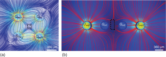
Figure 5.5 Numerically visualized flows and stagnation point/region of MQs. (a) 2D streamlines of the lateral MQ. Stagnation point visualized by divergence paths (black dotted square). (b) 2D streamlines and velocity profile of the linear MQ showing the stagnation region as the zero velocity regions (black dotted square).
5.4.2 Hydrodynamic Flow Confinement
To retain hydrodynamic confinement within the MQ, the gap between the MFP and the bottom substrate should be adequately small, and Qasp has to be sufficiently larger than Qin for all of the injected fluid to be re-aspirated. As injected chemicals may be used to process the underlying surface selectively [5], the confinement area of the MQ is of physical significance. For example, varying the flow rate ratio (Qasp/![]() from 1 to 8 with the lateral MQ, images of streaklines can be captured experimentally to visualize an increasing confinement effect (see Figure 5.6a–f). At Qasp/
from 1 to 8 with the lateral MQ, images of streaklines can be captured experimentally to visualize an increasing confinement effect (see Figure 5.6a–f). At Qasp/![]() , the lateral MQ is not fully confined as some of the injected fluid leaks out to the surrounding medium (see Figure 5.6a). As Qasp/Qin increases, the flow becomes more confined, and the area covered by the MQs reduces (see Figure 5.6b–f). The term used to characterize the area covered by the MQs is known as the confinement radius (R), defined as the distance between the stagnation point and the outermost point of zero velocity from the radial streams (see Figure 5.6c). This has been measured for various values of Qasp/Qin and shown to decay [3]. The hydrodynamic confinement has been shown to be preserved when scanning the MFP at low speeds, with slight disturbance in the shape [3]. At higher scanning speeds, this confinement breaks up and liquid leaks to the surrounding medium. However, this confined MQ shape proved to be recoverable in less than a second or so, depending on the operating flow rates and the gap between the MFP and the bottom substrate. Theoretical and numerical estimates of these features have also been shown to agree well with experimental measurements.
, the lateral MQ is not fully confined as some of the injected fluid leaks out to the surrounding medium (see Figure 5.6a). As Qasp/Qin increases, the flow becomes more confined, and the area covered by the MQs reduces (see Figure 5.6b–f). The term used to characterize the area covered by the MQs is known as the confinement radius (R), defined as the distance between the stagnation point and the outermost point of zero velocity from the radial streams (see Figure 5.6c). This has been measured for various values of Qasp/Qin and shown to decay [3]. The hydrodynamic confinement has been shown to be preserved when scanning the MFP at low speeds, with slight disturbance in the shape [3]. At higher scanning speeds, this confinement breaks up and liquid leaks to the surrounding medium. However, this confined MQ shape proved to be recoverable in less than a second or so, depending on the operating flow rates and the gap between the MFP and the bottom substrate. Theoretical and numerical estimates of these features have also been shown to agree well with experimental measurements.
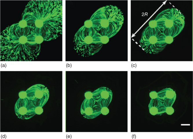
Figure 5.6 Flow confinement in the lateral MQ for varying Qasp/Qin. Tracer microbeads are injected at 50 nL/s. All experiments were captured with a 1 s exposure time. (a–f) Flow streaklines for Qasp/Qin = 1, 1.5, 1.75, 2, 4, 8, respectively. Scale bar is 360 µm.
5.4.3 Concentration Gradient Measurement
In order to experimentally visualize and measure the MQ's concentration gradient, fluorescein solution (fluorescein sodium salts diluted in water) was injected into one aperture of the MFP and deionized water through the other (see Figure 5.7a). Using the measured normalized fluorescent intensity, experimental measurements on the lateral MQ-generated concentration gradient was shown to match very well with numerical and analytical estimates [3]. Experimentally, this gradient takes just about 1 s to stabilize. The gradient length, arbitrarily defined as the distance between the points with concentration of 10% and 90% of the highest fluorescent signal on the acquired microscopic images, has been shown to decrease from 69 to 25.7 µm when Qin is maintained at 10 nL/s, while Qasp is varied from 20 to 250 nL/s [3]. Transient measurements show that the profile's slope changes rapidly with Qasp; however, varying Qin while keeping Qasp constant does not significantly change the profile's slope. As the aspiration flow rates are considerably higher than the injection flow rates for a fully confined MQ, it is anticipated that the gradient shape (advective vs diffusive mass transport) is highly dependent on the aspiration flow rates and slightly dependent on the injection flow rate. This suggests that by preprogramming Qasp/Qin, dynamic gradients can be readily produced, but the gradient's slope dependence is primarily on Qasp with high flow ratios (Qasp/Qin).

Figure 5.7 Concentration gradients formed with the MQ. (A) Images of the fluorescein distribution and concentration gradients within the lateral MQ. (B) Digital superimposition of the linear MQ's gradient image and the 2 µm green tracer bead flow field image showing the flow confinements of the injected chemicals and the gradient created in the stagnation region. Scale bars are 360 µm.
To experimentally visualize the concentration gradient with the linear MQ, a solution of 40 kDa dextran (red fluorescence; diffusion coefficient is 52.9 µm2/s) was injected from one of the inlet apertures, while only deionized water was injected through the other, with the surrounding immersion solution mixed with tracer beads [9]. Diffusion of the dextran solution through the stagnation region produces a visible gradient with a measurable intensity profile (see Figure 5.7b), which took about 15 min to establish and stabilize in this specific experiment. Normalizing the intensity profile over the distance a–b (shown in Figure 5.7b), a linear concentration can be observed, which validates the diffusion-dominated concentration gradient assumption. The observed concentration profile and linear intensity measurements have also been shown to match with the numerical calculations [9], see Figure 5.8.
5.4.4 Stagnation Point Hydrodynamic Manipulation
The stagnation point/region formed within the MQ is typically located on the X–X axis in the lateral MQ and on the Y–Y axis in the linear MQ (see Figure 5.8). When all flow rates are identical, X–X is located on the axis joining the center point of the aspiration apertures (stagnation point is located at the middle of the line), while Y–Y is located at the midline between the injection apertures. In addition, the concentration gradient is constant across the X–X axis in the lateral MQ (except at regions very close to the aspiration apertures), while the constant gradient region is formed in a curvature around the injection aperture in the linear MQ configuration. This is due to the counteraction on diffusive broadening by the dominating advective effects at locations away from the stagnation point and the focusing of stream by the concentric flow around the apertures. However, the position of these axes, and thus the location of the stagnation point, can be manipulated by modulating the aspiration flow ratio (Qasp1/Qasp2) and/or the injection flow ratio (Qin1/Qin2).
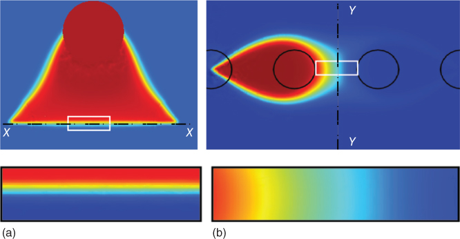
Figure 5.8 Numerically calculated concentration gradients of the lateral and linear MQs. (a) Concentration gradient of the lateral MQ. Enlarged view in the inset shows a constant concentration gradient along axis X–X. (b) Concentration gradient of the linear MQ. Inset showing concentration gradient across Y–Y. All aperture diameters are 360 µm.
Figure 5.9a,b shows that the position of the X–X axis of the lateral MQ varies from that of the axis connecting the midpoint of the aspiration apertures, which is the case when both aspiration and injection ratios are 1, to a nonsymmetrical and curved line, when the aspiration and injection ratios are 0.14 and 1.7, respectively. More complex landscapes of the dynamic gradient can be generated by similar adjustments, which can be automated for more precise control of the MQ's shape and the position of the stagnation point. Similarly, experiments with the linear MQ showed that the size of the stagnation region, and thus the concentration gradient, can be manipulated by modulating Qasp/Qin. When Qasp/Qin is increased, the confinement of injected fluids are stronger, and thus the stagnation region is bigger. In this case, the length of the concentration gradient is expected to be few times bigger. Figure 5.9c,d demonstrates this phenomenon as Qasp/Qin was increased from 3 to 10 in a linear MQ.
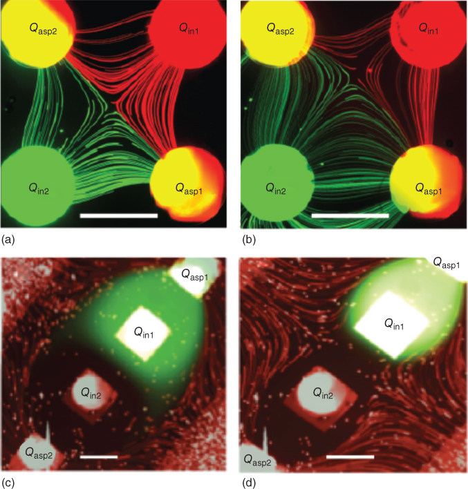
Figure 5.9 Dynamic concentration gradient within MQs. (a,b) A fluorescence micrograph of the lateral MQ showing streaklines of tracer microbeads following 2 s exposure with (a) Qin1 = Qin2 = 10 nL/s and Qasp1 = Qasp2= 100 nL/s, and (b) Qin1=  = 170 nL/s,
  . Transient measurements showed that the lateral MQ gradient could be moved and adjusted hydrodynamically. (c,d) A fluorescence micrograph of the linear MQ with fluorescein solution injected from one aperture, water from the other, and laced microbeads in the surrounding medium with (c) Qasp = 30 nL/s and Qin = 10 nL/s, and (d) Qasp= 100 nL/s and Qin= 10 nL/s. All scale bars are 360 µm.
5.5 Application of MQs in Biology and Life Sciences
5.5.1 MQs for Biochemical Concentration Gradient Assays
The ability of the MQ to generate reproducible, controllable, reconfigurable, and movable concentration gradients has numerous applications in cell chemotaxis studies and cell differentiation experiments. In vivo concentration gradients are essential to many biological processes and significantly contribute to cell development and response processes, which include growth guidance, migration, and differentiation of cells within living tissues [19]. Mimicking biochemical gradients in vitro presents an opportunity to replicate different biochemical gradients, to study their effects on cells, and to study how different molecular gradients impact different cell responses and sensitivities [19]. Such experiments can facilitate better understanding of cell microenvironments and cell–cell communications. Over the last 40 years, several traditional methods, and more recently microfluidic techniques, have been developed to generate in vitro concentration gradients for applications in cell studies [19]. These methods have been of great use and shaped our current understanding of in vivo microenvironments. The MQ's generated concentration gradients are associated with several unique characteristics in comparison with the traditional methods and other microfluidic techniques. These include the ability to scan over studied objects during experiments, the presence of a shear stress-free zone localized within the stagnation region, the system's characteristic open noncontacting configuration that allow for traditional cell culture protocols in Petri dishes and microtiter plates, and the ability to change the gradient shape and position during experiments. These make the MQ more applicable for cell dynamics studies during chemotaxis – under stationary and moving concentration gradients – as we will describe in the following section. In addition, the areas with minimal shear stresses within the MQ is favorable for studies interested in quantifying the shear stress effect on cells and tissues and in cases where shear stresses play an important role [4, 6]. A typical example of this is the transduction of applied shear stress stimulus by endothelial cells into intracellular responses in order to regulate the vessel structure [20]. Furthermore, the ability to apply concentration gradients to cells and tissues cultivated using the traditional cell culture protocols make the MQ well suited for studying cellular migrations [21, 22], neuronal navigation [23–25], and stem cell differentiation [26], as some cell types are very sensitive and have proven to be challenging to culture inside closed PDMS channels [27, 28]. In addition, concentration gradients can be applied to large biological samples such as tissue slices using the MQ, which is difficult to perform using closed channel microfluidic systems.
5.5.2 Studying Neutrophil Chemotaxis Using the Lateral MQ
Neutrophils are the most abundant type of white blood cells in humans and known as a very important component of the immune defense barrier against bacterial infections. They are highly dynamic and can reach the site of infections within minutes, with their activation considered as an indication of the presence of inflammation [29]. The process by which neutrophils migrate to the site of infection, in response to concentration gradients of various chemokines, is known as neutrophil chemotaxis [29]. Several techniques and methods have been developed and used to study this phenomenon [19, 30]; however, it is still not clear how neutrophils respond to moving gradients, and their dynamics during chemotaxis is not well understood.
The lateral MQ has been used to apply stationary and moving concentration gradients on a culture of human neutrophils in order to study their dynamics during chemotaxis [31, 32]. There are several chemokines that can induce neutrophil chemotaxis; however, interleukin 8 (IL-8) was used in the aforementioned study, as it is known to elicit strong neutrophil responses. Prior to the chemotaxis experiments, neutrophils were isolated from human blood by centrifugal density fractionation, stained with fluorescent dye, and cultured in Petri dishes. At the time of the chemotaxis assay, the neutrophil-containing plate was placed on the stage of the microscope, and the MQ was formed on the top of the cell culture, and consequently the concentration gradients were applied (see Figure 5.10a,b).
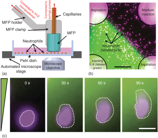
Figure 5.10 MQ application for neutrophil chemotaxis. (a) Experimental apparatus for applying concentration gradients to neutrophils using the lateral MQ [31]. (b) Fluorescent micrograph showing the generated IL-8 concentration gradients at the fluidic interface. The IL-8 solution is injected through the bottom left aperture, while medium is injected through the top right aperture. The other two apertures are used for aspirations. Neutrophils were labeled with eFluor670 proliferation dye (shown here in pink color) [32]. Scale bar is 200 µm. (c) Time-lapse micrographs of a single neutrophil polarizing within 30 s of applying the gradients and migrating to higher concentration in 60 s [32]. Scale bar is 10 µm.
Neutrophils were experimentally activated using the MQ, and their polarization and migration responses toward the higher concentration of the IL-8 chemokine were studied [31, 32]. The experiments showed that the migration speed of neutrophils is highest at the beginning of the MQ's gradient application and continuously decreases over time as the cells approach higher concentration of the chemokine IL-8. The study concluded that the migration length of neutrophils is correlated to their initial position within the stationary gradient, and experiments with moving gradients showed that neutrophils migrated longer distance, suggesting that neutrophils were pursuing the moving gradients [31, 32]. Interestingly, neutrophils were shown to react to the application of concentration gradient within only 30 s by changing their cellular shape (polarization) and started migrating toward the higher concentration of the gradient within only 1 min (see Figure 5.10c).
5.6 Summary and Outlook
The MQ is basically a microfluidic analogy of the typical electrical quadrupoles, with two pairs of opposing inlet and outlet apertures representing the positively and negatively charge fields, respectively. This can be achieved by arranging the apertures either in a lateral or linear configuration. The lateral MQ can be generated under an MFP with four apertures with alternating charged apertures arranged around the corners of a virtual square, while the linear MQ can be generated under an MFP with four apertures arranged on a straight line: two inner positively charged apertures (inlets) and two outer negatively charged apertures (outlets). The major differences between the lateral and linear MQs are the size of their stagnation and the time required to establish steady-state concentration gradients. Significant to the MQ is its ability to hydrodynamically form stress-free and tuneable stagnation regions and movable concentration gradients. The MQ allows for an open microfluidic platform, which not only solves the issues of the closed channel extensional flows but also comes with some added advantages. Laboratory measurements of these features have been carried out to proof the MQ's applicability in medical sciences, and numerical calculations have been used to substantiate observations.
The open MQ concept is still in its infancy [3]; as such, the technology is far from being a full-fledged product. Just as any new technology, the science behind this phenomenon has to be better understood for its practicality to become more evident; R&D undoubtedly has a significant role to play as a stimulus for commercialization. The MQ has three unique properties-dynamic nature, generation of a stagnation point/region, and ability to produce a concentration gradient – which suggests its applicability in capturing, enumerating, and characterizing biological particles, as well as scanning over biological samples and applying dynamic stimulations. These, in addition to its advantages over the closed chip extensional flows, portray the immense potential in biomedical scientific applications [8].
The dynamics of MQs present a good case for their application in capturing and stretching DNA molecules in order to ease the detection of target sequences under a microscope. In molecular biology, accurate prediction of DNA target sequences is fundamental to the understanding of many biological processes [33]. For example, in the transcription of genetic information from a DNA to a messenger RNA, transcription factors (TFs) [34] activate or repress gene expressions by using their DNA-binding domains (DBD) to attach specific DNA sequences in the genome [35]. Given that TFs are used for drug targets [36] and their mutations have been associated with some diseases in humans [37], accurate laboratory detection of DNA sequences is of significance in biomedicine. In order to detect target sequences on a DNA, the stagnation point of an MQ can be potentially used to trap DNA molecules, which can then be stretched by adjusting the system's Deborah number (De), a dimensionless ratio of DNA relaxation time and flow timescales that parameterize the flow strength and use fluorescence microscopy to measure the sequence [38]. In addition, akin to other extensional flow closed microfluidic chips [8], the MQ can also be used to trap cells in the stagnation region for studying cell growth and dynamics [39] and for studying cell deformability that represent a promising label-free diagnostic biomarker [40]. The MQ's stagnation point can also be utilized to study nonbiological objects such as polymer elasticity [41] and wormlike chains [42].
In a similar fashion, the open MQ's ability to hydrodynamically confine a concentration gradient has a particular interest in biomedicine assays; it can localize liquids on surfaces independent of the chemical composition of the confined liquids and without the need for electromigration of charged species. Basic adjustments of the MQ can be readily used to produce multiple layers of liquids shaped to get into contact with a surface, which have been demonstrated to be applicable in addressing critical aspects of microscale surface processing through minimal dilution, efficient retrieval, and fast switching of chemicals in a confined region [43].
In addition to these, the use of MQs for studying neutrophil chemotaxis is still evolving. Since the nature of chemokine gradients are mostly dynamic in the human body, it would be insightful to compare the dynamics of neutrophils activated by both stationary and moving concentration gradients of IL-8, generated by an MQ. Also, different speeds and directions of the moving gradients can be tested, in a preprogrammed manner, or with a predefined feedback system that can track the cell movement and adjust the position of the gradient accordingly. The migration of cancer cells, growth cones and axonal navigation of neurons, and stem cell differentiation can be studied as well. This could potentially shape our understanding of chemokine signaling and cell patterning during development.
The ultimate aim of most researchers in the microfluidic field is to develop technologies, which would transit from being topics in research articles to becoming a full-scale clinical device in the form of lab-on-chip devices. This is also the future we envisage for the MQ. However, the commercial success of lab-on-chip devices, and hence that of the MQ, is highly reliant on how much they can simplify an otherwise tedious process, with a high level of sensitivity and throughput [44, 45]. These devices are usually designed to solve bottom-top problems for users with little or no expertise in the physics involved. In order for the MQ to facilitate such, its dependence on external devices for automation needs to be addressed. Methods of automatically adjusting the outlet flow in situ, so as to manipulate the position of the stagnation point and the generated concentration gradient, are necessary. It is only after this it would be feasible to integrate with other microfluidic techniques for a full-fledged lab-on-chip device.
References
- 1 Wiedemann, H. (1999) Particle accelerator physics I, in Basic Principles and Linear Beam Dynamics, Springer-Verlag, p. 469.
- 2 DeHoffmann, H. and Stroobant, V. (2007) Mass Spectrometry: Principles and Applications, John Wiley & Sons, p. 503.
- 3 Qasaimeh, M.A., Gervais, T., and Juncker, D. (2011) Microfluidic quadrupole and floating concentration gradient. Nat. Commun., 2, 464.
- 4 Qasaimeh, M.A., Ricoult, S.G., and Juncker, D. (2013) Microfluidic probes for use in life sciences and medicine. Lab Chip, 13, 40–50.
- 5 Juncker, D., Schmid, H., and Delamarche, E. (2005) Multipurpose microfluidic probe. Nat. Mater., 4, 622–628.
- 6 Safavieh, M., Qasaimeh, M.A., Vakil, A., Juncker, D., and Gervais, T. (2015) Two-aperture microfluidic probes as flow dipoles: theory and applications. Sci. Rep., 5. doi: 10.1038/srep11943
- 7 Macosko, C.W., Ocansey, M.A., and Winter, H.H. (1982) Steady planar extensions with lubricated dies. J. Non-Newtonian Fluid Mech., 11, 301–316.
- 8 Brimmo, A.T. and Qasaimeh, M.A. (2017) Stagnation point flows in analytical chemistry and life sciences. RSC Advances, 7 (81), 51206–51232.
- 9 Qasaimeh, M., Stefavieh, R., and Juncker, D. (2009) The generation of biochemical gradients in a microfluidic stagnant zone. The 5th International Conference on Microtechnologies in Medicine and Biotechnologies, Quebec, Canada.
- 10 King, K.R., Wang, S., Jayaraman, A., Yarmush, M.L., and Toner, M. (2008) Microfluidic flow-encoded switching for parallel control of dynamic cellular microenvironments. Lab Chip, 8, 107–116.
- 11 Takayama, S., Ostuni, E., LeDuc, P., Naruse, K., Ingber, D., and Whitesides, G. (2003) Selective chemical treatment of cellular microdomains using multiple laminar streams. Chem. Biol., 10 (2), 123–130.
- 12 Tanyeri, M., Johnson-Chavarria, E.M., and Schroeder, C.M. (2010) Hydrodynamic trap for single particles and cells. Appl. Phys. Lett., 96 (22), 224101.
- 13 Johnson-Chavarria, E., Agrawal, U., Tanyeri, M., and Schroeder, C.M. (2011) Microfluidic-based trap for single cell micromanipulation and analysis. Biophys. J., 100 (3), 623a.
- 14 Tanyeri, M. and Schroeder, C.M. (2013) Manipulation and confinement of single particles using fluid flow. Nano Lett., 13 (6), 2357–2364.
- 15 Tanyeri, M. and Schroeder, C.M. (2014) Flow-based particle trapping and manipulation, in Encyclopedia of Microfluidics and Nanofluidics (ed. D. Li), Springer US, pp. 1–9.
- 16 Shenoy, A., Tanyeri, M., and Schroeder, C.M. (2014) Characterizing the performance of the hydrodynamic trap using a control-based approach. Microfluid. Nanofluid., 18 (5–6), 1055–1066.
- 17 Perrault, C.M., Qasaimeh, M.A., Brastaviceanu, T., Anderson, K., Kabakibo, Y., and Juncker, D. (2010) Integrated microfluidic probe station. Rev. Sci. Instrum., 81, 115107.
- 18 Hitzbleck, M., Kaigala, G.V., Delamarche, E., and Lovchik, R.D. (2014) The floating microfluidic probe: distance control between probe and sample using hydrodynamic levitation. Appl. Phys. Lett., 104, 263501.
- 19 Irimia, D. (2010) Microfluidic technologies for temporal perturbations of chemotaxis. Annu. Rev. Biomed. Eng., 15 (12), 259–284.
- 20 Chachisvilis, M., Zhang, Y., and Frangos, J. (2006) G protein-coupled receptors sense fluid shear stress in endothelial cells. Proc. Natl. Acad. Sci. U.S.A., 103 (42), 15463–15468.
- 21 Jeon, N.L., Baskaran, H., Dertinger, S.K.W., Whitesides, G.M., Van De Water, L., and Toner, M. (2002) Neutrophil chemotaxis in linear and complex gradients of interleukin-8 formed in a microfabricated device. Nat. Biotechnol., 20 (8), 826–830.
- 22 Cosson, S., Kobel, S., and Lutolf, M. (2009) Capturing complex protein gradients on biomimetic hydrogels for cell-based assays. Adv. Funct. Mater., 19 (21), 3411–3419.
- 23 Dertinger, S., Jiang, X., Li, Z., Murthy, V., and Whitesides, G. (2002) Gradients of substrate-bound laminin orient axonal specification of neurons. Proc. Natl. Acad. Sci. U. S. A., 99 (20), 12542–12547.
- 24 Yam, P., Langlois, S., Morin, S., and Charron, F. (2009) Sonic hedgehog guides axons through a noncanonical, Src-family-kinase-dependent signaling pathway. Neurons, 62 (3), 349–362.
- 25 Sloan, T.F.W., Qasaimeh, M.A., Juncker, D., Yam, P.T., and Charron, F. (2015) Integration of shallow gradients of Shh and Netrin-1 guides commissural axons. PLoS Biol., 13 (3), e1002119.
- 26 Wu, H., Lin, C., and Lee, G. (2011) Stem cells in microfluidics. Biomicrofluidics, 5 (1), 013401.
- 27 Regehr, K., Domenech, M., Koepsel, J., Carver, K., Ellison-Zelski, S., Murphy, W., Schuler, L., Alarid, E., and Beebe, D. (2009) Biological implications of polydimethylsiloxane-based microfluidic cell culture. Lab Chip, 9 (15), 2132–2139.
- 28 Millet, L., Stewart, M., Sweedler, J., Nuzzo, R., and Gillette, M. (2007) Microfluidic devices for culturing primary mammalian neurons at low densities. Lab Chip, 7 (8), 987–994.
- 29 Kolaczkowska, E. and Kubes, P. (2013) Neutrophil recruitment and function in health and inflammation. Nat. Rev. Immunol., 13 (3), 159–175.
- 30 Keenan, T. and Folch, A. (2008) Biomolecular gradients in cell culture systems. Lab Chip, 8 (1), 34–57.
- 31 Qasaimeh, M.A., Astolfi, M., Pyzik, M., Vidal, S., and Juncker, D. (2014) Neutrophil dynamics during migration in microfluidic concentration gradients. 2014 40th Annual Northeast, Bioengineering Conference (NEBEC), Boston, MA.
- 32 Qasaimeh, M.A., Astolfi, M., Pyzik, M., Vidal, S., and Juncker, D. (2013) Neutrophils migrate longer distances in moving microfluidic concentration gradients compared to static ones. The 17th International Conference on Miniaturized Systems for Chemistry and Life Sciences (microTAS), Freiburg, Germany.
- 33 Chen, C.C., Chien, T.Y., Lin, C.K., Lin, C.W., Weng, Y.Z., and Chang, D.T. (2012) Predicting target DNA sequences of DNA-binding proteins based on unbound structures. PLoS One, 7 (2), e30446.
- 34 Latchman, D.S. (1997) Transcription factors: an overview. Int. J. Biochem. Cell Biol., 29 (12), 1305–1312.
- 35 Mitchell, P. and Tijan, T. (1989) Transcriptional regulation in mammalian cells by sequence-specific DNA binding proteins. Science, 245 (4916), 371–378.
- 36 Overington, J.P., Al-Lazikani, B., and Hopkins, A.L. (2006) How many drug targets are there? Nat. Rev. Drug Recovery, 5 (12), 993–996.
- 37 Semanza, G.L. (1999) Transcription Factors and Human Disease, Oxford University Press, Oxfordshire.
- 38 Dylla-Spears, R., Townsend, J.E., Jen-Jacobson, L., Sohn, L.L., and Muller, S.J. (2010) Single-molecule sequence detection via microfluidic planar extensional flow at a stagnation point. Lab Chip, 10 (12), 1543–1549.
- 39 Johnson-Chavarria, E.M., Agrawal, U., Tanyeri, M., Kuhlmanac, T.E., and Schroeder, C.M. (2014) Automated single cell microbioreactor for monitoring intracellular dynamics and cell growth in free solution. Lab Chip, 14 (15), 2688–2697.
- 40 Cha, S., Shin, T., Lee, S.S., Shim, W., Lee, G., Lee, S.J., Kim, Y., and Kim, J.M. (2012) Cell stretching measurement utilizing viscoelastic particle focusing. Anal. Chem., 84 (33), 10471–10477.
- 41 Latinwo, F. and Schroeder, C.M. (2014) Determining elasticity from single polymer dynamics. Soft Matter, 10 (13), 2178–2187.
- 42 Li, X., Schroeder, C.M., and Dorfman, K.D. (2015) Modeling the stretching of wormlike chains in the presence of excluded volume. Soft Matter, 11 (29), 5947–5954.
- 43 Autebert, J., Kashyap, A., Lovchik, R.D., Delamarche, E., and Kaigala, G.V. (2014) Hierarchical hydrodynamic flow confinement: efficient use and retrieval of chemicals for microscale chemistry on surfaces. Langmuir, 13 (12), 3640–3645.
- 44 Whitesides, G.M. (2006) The origins and future of microfluidics. Nature, 442, 368–373.
- 45 Kim, Y.T. and Langer, R. (2015) Microfluidics in nanomedicine. Rev. Cell Biol. Mol. Med., 1, 127–152.