
In this recipe, we'll take a look at the basics of tessellation shaders by drawing a cubic Bezier curve. A Bezier curve is a parametric curve defined by four control points. The control points define the overall shape of the curve. The first and last of the four points define the start and end of the curve, and the middle points guide the shape of the curve, but do not necessarily lie directly on the curve itself. The curve is defined by interpolating the four control points using a set of blending functions. The blending functions define how much each control point contributes to the curve for a given position along the curve. For Bezier curves, the blending functions are known as the Bernstein polynomials.
In the preceding equation, the first term is the binomial coefficient function (shown in the following equation), n is the degree of the polynomial, i is the polynomial number, and t is the parametric parameter.

The general parametric form for the Bezier curve is then given as a sum of the products of the Bernstein polynomials with the control points (P i).

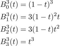
In this example, we will draw a cubic Bezier curve, which involves four control points (n = 3).
And the cubic Bernstein polynomials are:
As stated in the introduction of this chapter, the tessellation functionality within OpenGL involves two shader stages. They are the tessellation control shader (TCS) and the tessellation evaluation shader (TES). In this example, we'll define the number of line segments for our Bezier curve within the TCS (by defining the outer tessellation levels), and evaluate the Bezier curve at each particular vertex location within the TES. The following screenshot shows the output of this example for three different tessellation levels. The left figure uses three line segments (level 3), the middle uses level 5, and the right-hand figure is created with tessellation level 30. The small squares are the control points.

The control points for the Bezier curve are sent down the pipeline as a patch primitive consisting of four vertices. A patch primitive is a programmer-defined primitive type. Basically, it is a set of vertices that can be used for anything that the programmer chooses. The TCS is executed once for each vertex within the patch, and the TES is executed, a variable number of times, depending on the number of vertices produced by the TPG. The final output of the tessellation stages is a set of primitives. In our case, it will be a line strip.
Part of the job for the TCS is to define the tessellation level. In very rough terms, the tessellation level is related to the number of vertices that will be generated. In our case, the TCS will be generating a line strip, so the tessellation level is the number of line segments in the line strip. Each vertex that is generated for this line strip will be associated with a tessellation coordinate that will vary between zero and one. We'll refer to this as the u coordinate, and it will correspond to the parametric parameter t in the preceding Bezier curve equation.
Note
What we've looked at so far is not, in fact, the whole story. Actually, the TCS will trigger a generation of a set of line strips called isolines. Each vertex in this set of isolines will have a u and a v coordinate. The u coordinate will vary from zero to one along a given isoline, and v will be constant for each isoline. The number of distinct values of u and v is associated with two separate tessellation levels, the so-called "outer" levels. For this example, however, we'll only generate a single line strip, so the second tessellation level (for v) will always be one.
Within the TES, the main task is to determine the position of the vertex associated with this execution of the shader. We have access to the u and v coordinates associated with the vertex, and we also have (read-only) access to all of the vertices of the patch. We can then determine the appropriate position for the vertex by using the parametric equation described above, with u as the parametric coordinate (t in the preceding equation).
The following are the important uniform variables for this example:
NumSegments: This is the number of line segments to be produced.NumStrips: This is the number of isolines to be produced. For this example, this should be set to one.LineColor: This is the color for the resulting line strip.
Set the uniform variables within the main OpenGL application. There are a total of four shaders to be compiled and linked. They are the vertex, fragment, tessellation control, and tessellation evaluation shaders.
To create a shader program that will generate a Bezier curve from a patch of four control points, use the following steps:
- Use the following code for the simple vertex shader:
layout (location = 0 ) in vec2 VertexPosition; void main() { gl_Position = vec4(VertexPosition, 0.0, 1.0); } - Use the following code as the tessellation control shader:
layout( vertices=4 ) out; uniform int NumSegments; uniform int NumStrips; void main() { // Pass along the vertex position unmodified gl_out[gl_InvocationID].gl_Position = gl_in[gl_InvocationID].gl_Position; // Define the tessellation levels gl_TessLevelOuter[0] = float(NumStrips); gl_TessLevelOuter[1] = float(NumSegments); } - Use the following code as the tessellation evaluation shader:
layout( isolines ) in; uniform mat4 MVP; // projection * view * model void main() { // The tessellation u coordinate float u = gl_TessCoord.x; // The patch vertices (control points) vec3 p0 = gl_in[0].gl_Position.xyz; vec3 p1 = gl_in[1].gl_Position.xyz; vec3 p2 = gl_in[2].gl_Position.xyz; vec3 p3 = gl_in[3].gl_Position.xyz; float u1 = (1.0 - u); float u2 = u * u; // Bernstein polynomials evaluated at u float b3 = u2 * u; float b2 = 3.0 * u2 * u1; float b1 = 3.0 * u * u1 * u1; float b0 = u1 * u1 * u1; // Cubic Bezier interpolation vec3 p = p0 * b0 + p1 * b1 + p2 * b2 + p3 * b3; gl_Position = MVP * vec4(p, 1.0); } - Use the following code for the fragment shader:
uniform vec4 LineColor; layout ( location = 0 ) out vec4 FragColor; void main() { FragColor = LineColor; } - It is important to define the number of vertices per patch within the OpenGL application. You can do so using the
glPatchParameterfunction:glPatchParameteri( GL_PATCH_VERTICES, 4);
- Render the four control points as a patch primitive within the OpenGL application's render function:
glDrawArrays(GL_PATCHES, 0, 4);
The vertex shader is just a "pass-through" shader. It sends the vertex position along to the next stage without any modification.
The tessellation control shader begins by defining the number of vertices in the output patch:
layout (vertices = 4) out;
Note that this is not the same as the number of vertices that will be produced by the tessellation process. In this case, the patch is our four control points, so we use a value of four.
The main method within the TCS passes the input position (of the patch vertex) to the output position without modification. The arrays gl_out and gl_in contain the input and output information associated with each vertex in the patch. Note that we assign and read from location gl_InvocationID in these arrays. The gl_InvocationID variable defines the output patch vertex for which this invocation of the TCS is responsible. The TCS can access all of the array gl_in, but should only write to the location in gl_out corresponding to gl_InvocationID.
Next, the TCS sets the tessellation levels by assigning to the gl_TessLevelOuter array. Note that the values for gl_TessLevelOuter are floating point numbers rather than integers. They will be rounded up to the nearest integer and clamped automatically by the OpenGL system.
The first element in the array defines the number of isolines that will be generated. Each isoline will have a constant value for v. In this example, the value of gl_TessLevelOuter[0] should be one. The second defines the number of line segments that will be produced in the line strip. Each vertex in the strip will have a value for the parametric u coordinate that will vary from zero to one.
In the TES, we start by defining the input primitive type using a layout declaration:
layout (isolines) in;
This indicates the type of subdivision that is performed by the tessellation primitive generator. Other possibilities here include quads and triangles.
Within the main function of the TES, the variable gl_TessCoord contains the tessellation u and v coordinates for this invocation. As we are only tessellating in one dimension, we only need the u coordinate, which corresponds to the x coordinate of gl_TessCoord.
The next step accesses the positions of the four control points (all the points in our patch primitive). These are available in the gl_in array.
The cubic Bernstein polynomials are then evaluated at u and stored in b0, b1, b2, and b3. Next, we compute the interpolated position using the Bezier curve equation described some time back. The final position is converted to clip coordinates and assigned to the output variable gl_Position.
The fragment shader simply applies LineColor to the fragment.