
In this recipe, we'll implement a simple particle simulation. We'll have the compute shader handle the physics computations and update the particle positions directly. Then, we'll just render the particles as points. Without the compute shader, we'd need to update the positions on the CPU by stepping through the array of particles and updating each position in a serial fashion, or by making use of transform feedback as shown in the Creating a particle system using transform feedback recipe in Chapter 9, Particle Systems and Animation. Doing such animations with vertex shaders is sometimes counterintuitive and requires some additional work (such as transform feedback setup). With the compute shader, we can do the particle physics in parallel on the GPU, and customize our compute space to get the most "bang for the buck" out of our GPU.
The following figure shows our particle simulation running with one million particles. Each particle is rendered as a 1 x 1 point. The particles are partially transparent, and the particle attractors are rendered as small 5 x 5 squares (barely visible).
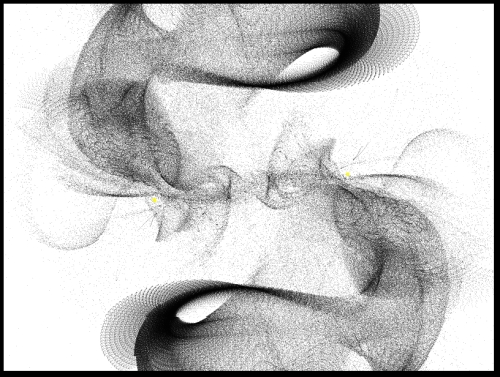
These simulations can create beautiful, abstract figures, and are a lot of fun to produce.
For our simulation, we'll define a set of attractors (two in this case, but you can create more), which I'll call the black holes. They will be the only objects that affect our particles and they'll apply a force on each particle that is inversely proportional to the distance between the particle and the black hole. More formally, the force on each particle will be determined by the following equation:
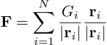
Where N is the number of black holes (attractors), ri is the vector between the ith attractor and the particle (determined by the position of the attractor minus the particle position), and Gi is the strength of the ith attractor.
To implement the simulation, we compute the force on each particle and then update the position by integrating the Newtonian equations of motion. There are a number of well studied numerical techniques for integrating the equations of motion. For this simulation, the simple Euler method is sufficient. With the Euler method, the position of the particle at time t + Δt is given by the following equation:
Where P is the position of the particle, v is the velocity, and a is the acceleration. Similarly, the updated velocity is determined by the following equation:
These equations are derived from a Taylor expansion of the position function about time t. The result is dependent upon the size of the time step (Δt), and is more accurate when the time step is very small.
The acceleration is directly proportional to the force on the particle, so by calculating the force on the particle (using the preceding equation), we essentially have a value for the acceleration. To simulate the particle's motion, we track its position and velocity, determine the force on the particle due to the black holes, and then update the position and velocity using the equations.
We'll use the compute shader to implement the physics here. Since we're just working with a list of particles, we'll use a one-dimensional compute space, and work groups of about 1000 particles each. Each invocation of the compute shader will be responsible for updating the position of a single particle.
We'll use shader storage buffer objects to track the positions and velocities, and when rendering the particles themselves, we can just render directly from the position buffer.
In the OpenGL side, we need a buffer for the position of the particles and a buffer for the velocity. Create a buffer containing the initial positions of the particles and a buffer with zeroes for the initial velocities. We'll use four-component positions and velocities for this example in order to avoid issues with data layouts. For example, to create the buffer for the positions, we might do something as follows:
vector<GLfloat> initPos;

… // Set initial positions

GLuint bufSize = totalParticles * 4 * sizeof(GLfloat);

GLuint posBuf;
glGenBuffers(1, &posBuf);
glBindBufferBase(GL_SHADER_STORAGE_BUFFER, 0, posBuf);
glBufferData(GL_SHADER_STORAGE_BUFFER, bufSize, &initPos[0],
               GL_DYNAMIC_DRAW);
Use a similar process for the velocity data, but bind it to index one of the GL_SHADER_STORAGE_BUFFER binding location.
glBindBufferBase(GL_SHADER_STORAGE_BUFFER, 1, velBuf);
Set up a vertex array object that uses the same position buffer as its data source for the vertex position.
To render the points, set up a vertex and fragment shader pair that just produces a solid color. Enable blending and set up a standard blending function.
Use the following steps:
- We'll use the compute shader for updating the positions of the particles.
layout( local_size_x = 1000 ) in; uniform float Gravity1 = 1000.0; uniform vec3 BlackHolePos1; uniform float Gravity2 = 1000.0; uniform vec3 BlackHolePos2; uniform float ParticleInvMass = 1.0 / 0.1; uniform float DeltaT = 0.0005; layout(std430, binding=0) buffer Pos { vec4 Position[]; }; layout(std430, binding=1) buffer Vel { vec4 Velocity[]; }; void main() { uint idx = gl_GlobalInvocationID.x; vec3 p = Position[idx].xyz; vec3 v = Velocity[idx].xyz; // Force from black hole #1 vec3 d = BlackHolePos1 - p; vec3 force = (Gravity1 / length(d)) * normalize(d); // Force from black hole #2 d = BlackHolePos2 - p; force += (Gravity2 / length(d)) * normalize(d); // Apply simple Euler integrator vec3 a = force * ParticleInvMass; Position[idx] = vec4( p + v * DeltaT + 0.5 * a * DeltaT * DeltaT, 1.0); Velocity[idx] = vec4( v + a * DeltaT, 0.0); } - In the render routine, invoke the compute shader to update the particle positions.
glDispatchCompute(totalParticles / 1000, 1, 1);
- Then make sure that all data has been written out to the buffer, by invoking a memory barrier.
glMemoryBarrier( GL_SHADER_STORAGE_BARRIER_BIT );
- Finally, render the particles using data in the position buffer.
The compute shader starts by defining the number of invocations per work group using the layout specifier.
layout( local_size_x = 1000 ) in;
This specifies 1000 invocations per work group in the x dimension. You can choose a value for this that makes the most sense for the hardware on which you're running. Just make sure to adjust the number of work groups appropriately. The default size for each dimension is one so we don't need to specify the size of the y and z directions.
Then, we have a set of uniform variables that define the simulation parameters. Gravity1 and Gravity2 are the strengths of the two black holes (G in the above equation), and BlackHolePos1 and BlackHolePos2 are their positions. ParticleInvMass is the inverse of the mass of each particle, which is used to convert force to acceleration. Finally, DeltaT is the time-step size, used in the Euler method for integration of the equations of motion.
The buffers for position and velocity are declared next. Note that the binding values here match those that we used on the OpenGL side when initializing the buffers.
Within the main function, we start by determining the index of the particle for which this invocation is responsible. Since we're working with a linear list of particles, and the number of particles is the same as the number of shader invocations, what we want is the index within the global range of invocations. This index is available via the built-in input variable gl_GlobalInvocationID.x. We use the global index here because it is the index within the entire buffer that we need, not the index within our work group, which would only reference a portion of the entire array.
Next we retrieve the position and velocity from their buffers, and compute the force due to each black hole, storing the sum in the variable force. Then we convert the force to acceleration and update the particle's position and velocity using the Euler method. We write to the same location from which we read previously. Since invocations do not share data, this is safe.
In the render routine, we invoke the compute shader (step 2 in How to do it...), defining the number of work groups per dimension. In the compute shader, we specified a work group size of 1000. Since we want one invocation per particle, we divide the total number of particles by 1000 to determine the number of work groups.
Finally, in step 3, before rendering the particles, we need to invoke a memory barrier to ensure that all compute shader writes have fully executed.
- Refer to Chapter 9, Particle Systems and Animation, for other particle simulations. Most of these have been implemented using transform feedback, but could instead be implemented using the compute shader.