The final step after creating the model is to use the model against the test dataset to get the predictions. This is generally done using the predict function in R, with the first argument being the model that was created and the second argument being the dataset against which you'd like to get the predictions for.

Taking our example of the PimaIndiansDiabetes dataset, after the model has been built, we can get the predictions on the test dataset as follows:

# Install the R Package e1071, if you haven't already 
# By running install.packages("e1071") 
 
# Use the predict function and the rf_model that was previously built 
# To get the predictions on the test dataset 
# Note that we are not including the column diabetes in the test 
# dataset by using diab_test[,-ncol(diab_test)] 
 
predictions<- predict(rf_model, diab_test[,-ncol(diab_test)]) 
 
# First few records predicted 
head(predictions)
[1] negnegpospospospos 
Levels: negpos 
 
# The confusion matrix allows us to see the number of true positives 
# False positives, True negatives and False negatives 
 
cf<- confusionMatrix(predictions, diab_test$diabetes) 
cf 
 
# Confusion Matrix and Statistics 
#  
#        Reference 
# Prediction negpos 
#        neg  89  21 
#        pos  11  32 
#  
# Accuracy : 0.7908           
# 95% CI : (0.7178, 0.8523) 
# No Information Rate : 0.6536           
# P-Value [Acc> NIR] : 0.0001499        
#  
# Kappa : 0.5167           
# Mcnemar's Test P-Value : 0.1116118        
#  
# Sensitivity : 0.8900           
# Specificity : 0.6038           
# PosPredValue : 0.8091           
# NegPredValue : 0.7442           
# Prevalence : 0.6536           
# Detection Rate : 0.5817           
# Detection Prevalence : 0.7190           
# Balanced Accuracy : 0.7469           
#  
# 'Positive' Class :neg 

Let's check what the confusion matrix tells us:

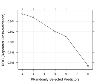
# This indicates that of the records that were marked negative (neg) 
# We predicted 89 of them as negative and 11 as positive (i.e., they 
# were negative but we incorrectly classified them as a positive 
 
# We correctly identified 32 positives but incorrectly classified 
# 21 positives as negative 
 
# 
#           Reference 
# Prediction neg  pos 
#        neg  89  21 
#        pos  11  32 
 
# The overall accuracy was 79% 
# This can be improved (significantly) by using more  
# Accuracy : 0.7908           
 
# We can plot the model using plot(rf_model) as follows 
plot(rf_model) 

The plot is as follows:

# And finally we can also visualize our confusion matrix using the 
# inbuilt fourfoldplot function in R 
 
fourfoldplot(cf$table) 

We get the plot as follows: