K-Means is one of the most popular unsupervised machine learning techniques that is used to create clusters, and so categorizes data.

An intuitive example could be posed as follows:

Say a university was offering a new course on American History and Asian History. The university maintains a 15:1 student-teacher ratio, so there is 1 teacher per 15 students. It has conducted a survey which contains a 10-point numeric score that was assigned by each student to their preference of studying American History or Asian History.

We can use the in-built K-Means algorithm in R to create 2 clusters and presumably, by the number of points in each cluster, it may be possible to get an estimate of the number of students who may sign up for each course. The code for the same is given as follows:

library(data.table) 
library(ggplot2) 
library() 
 
historyData<- fread("~/Desktop/history.csv") 
ggplot(historyData,aes(american_history,asian_history)) + geom_point() + geom_jitter() 
 
historyCluster<- kmeans(historyData,2) # Create 2 clusters 
historyData[,cluster:=as.factor(historyCluster$cluster)] 
ggplot(historyData, aes(american_history,asian_history,color=cluster)) + geom_point() + geom_jitter()

# The image below shows the output of the ggplot command. Note that the effect of geom_jitter can be seen in the image below (the points are nudged so that overlapping points can be easily visible)

The following image could provide an intuitive estimate of the number of students who may sign up for each course (and thereby determine how many teachers may be required):

There are several variations of the K-Means algorithm, but the standard and the most commonly used one is Lloyd's Algorithm. The algorithm steps are as follows:

Given a set of n points (say in an x-y axis), in order to find k clusters:

1. Select k points at random from the dataset to represent the mid-points for k clusters (say, the initial centroids).
2. The distance from each of the other points to the selected k points (representing k clusters) is measured and assigned to the cluster that has the lowest distance from the point.
3. The cluster centers are recalculated as the mean of the points in the cluster.
4. The distance between the centroids and all the other points are again calculated as in Step 2 and new centroids are calculated as in Step 3. In this manner, Steps 2 and 3 are repeated until no new data is re-assigned.

Various distance and similarity measures exist for clustering, such as Euclidean Distance (straight-line distance), Cosine Similarity (Cosine of angles between vectors), Hamming Distance (generally used for categorical variables), Mahalanobis Distance (named after P.C. Mahalanobis; this measures the distance between a point and the mean of a distribution), and others.

Although the optimal number of clusters cannot always be unambiguously identified, there are various methods that attempt to find an estimate. In general, clusters can be measured by how close points within a cluster are to one another (within cluster variance, such as the sum of squares--WSS) and how far apart the clusters are (so higher distances between clusters would make the clusters more readily distinguishable). One such method that is used to determine the optimal number is known as the elbow method. The following chart illustrates the concept:

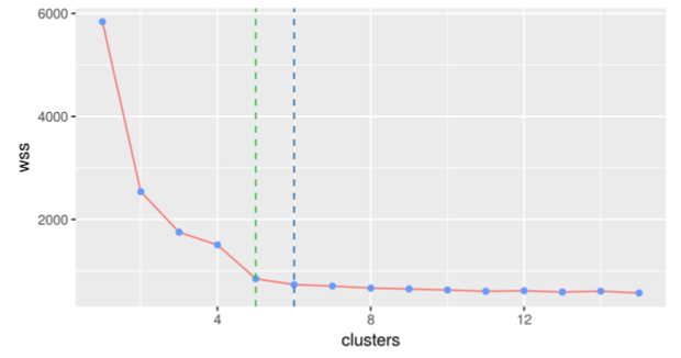
The chart shows a plot of the WSS (within the cluster sum of squares that we're seeking to minimize) versus the number of clusters. As is evident, increasing the number of clusters from 1 to 2 decreases the WSS value substantially. The value for WSS decreases rapidly up until the 4^th or 5^th cluster, when adding more clusters does not lead to a significant improvement in WSS. By visual assessment, the machine learning practitioner can conclude that the ideal number of clusters that can be created is between 3-5, based on the image.