2.2 CFA Model with Continuous Indicators

Having introduced the basic concepts of CFA models, let us turn our attention to application of CFA with continuous indicators in the framework of the Mplus program. In this section, we demonstrate how to run the example CFA model proposed in Section 2.1 using real data. Data used here are from a natural history study of rural illicit drug users in Ohio, USA. Such a population is an important population for testing BSI- 18, given the high rates of psychiartric distress both as a consequence of their drug use and as a pre- existing condition for which they are self- medicating (Grant et al., 2004). A total sample of 248 drug users was recruited from three rural counties in Ohio: respondent- driven sampling (RDS) was used for sample recruitment (Heckathorn, 1997, 2002; Wang et al., 2007). A detailed description on recruitment approaches and sample characteristics can be found in the literature (Siegal et al., 2006).

Recall that the responses to the BSI- 18 items are measured on a five- point Likert scale: 0, not at all; 1, a little bit; 2, moderately; 3, quite a bit; and 4, extremely. Although they are actually ordinal scales, Likert scales are often treated as numeric measures in CFA, as well as in other statistical modeling. We will treat the observed indicators as numeric and ordinal measures, respectively, and recode them as binary measures for the purpose of model demonstrations. The following Mplus program or syntax file estimates a three- factor (i.e., SOM, DEP, and ANT) CFA model, in which all the BSI- 18 items are treated as continuous indicators.

Mplus Program 2.1

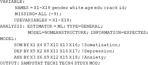
where TITLE command provides a label for the program. Although it is optional, it is always a good idea to give some notes in the TITLE command. The DATA command tells the program where to read the data. The data are in ASCII (American Standard Code for Information Interchange) format or text format. The FILE statement in the DATA command specifies the data file name. In our example, both the data file (BSI_18.dat) and program file (Mplus inp) are stored in the same folder on our computer, thus path specification is not necessary here. The LISTWISE = ON statement specifies a LISTWISE⁷ missing value deletion, which is also called CASEWISE deletion. That is, if a case has missing values on any of the variables, it will be dropped completely from analysis.

In the VARIABLE command, the statement NAMES specifies all the variable names included in the data. Note that the order of the variables specified in the program must match the order they appear in the data. Only these variables that are used in the model are specified in the USEVARIABLES statement where the order of variables does not matter in this line of code. But note that all selected variables must be used in the model. In this example, variables x1 − x18 in the data set are used for modeling. The MISSING statement specifies any user- specified missing values in the data. For example, missing values in the data are coded as - 9 and specified by ‘ MISSING = ALL (− 9); ’ in the VARIABLE command. Missing values can also be coded as ‘.’ and specified by ‘MISSING = ALL.’ or ‘MISSING =.;’ in the VARIABLE command.

The ANALYSIS command specifies what type of analysis will be implemented. For example, the default is TYPE = GENERAL that covers analyses included in the Mplus Base Program, such as regression, path analysis, CFA, SEM, growth modeling, and survival analysis, while TYPE = MIXTURE is required for mixture modeling; and TYPE = TWOLEVEL for multilevel modeling. In addition, different estimators can be specified in the ANALYSIS command for model estimation. When the observed indicators are continuous measures, the default estimator is the ML estimator. The statements MODEL = NOMEANSTRUCTURE and INFORMATION = EXPECTED in the ANALYSIS command tell the program to analyze covariance structures (COVS) in the modeling. As aforementioned, traditionally the observed variables are measured in deviations from their means, and COVS is analyzed in SEM. This data transformation helps simplify model specification and calculation, and does not affect parameter estimation. However, when factor means and indicator intercepts (or thresholds of categorical indicators) are concerned in the model, the mean and covariance structures (MACS) should be analyzed. This is also called analysis of moment structures. Most of the SEM programs estimate CFA and SEM under COVS by default. Starting from version 5, Mplus sets MACS as the default. In order to estimate model under COVS, statements MODEL = NOMEANSTRUCTURE and INFORMATION = EXPECTED must be specified in the ANALYSIS command of the Mplus program.

The model is specified in the MODEL command. In our example, the 18 indicators are loaded on three factors (SOM, DEP, and ANX) via the BY statements. The factor loadings for the first indicator of each factor are fixed to 1.0 by default for the purpose of model identification.

In the OUTPUT command, the SAMPSTAT statement allows sample statistics to be printed in the output file; TECH1 reports parameter specification; TECH4 prints variances, covariances, and correlations among the latent variables/factors; STDYX requests complete standardization solution; ⁸ and MOD prints MIs.

There are a few tips in Mplus programming. First, if no folder/directory is specified for the data file in the DATA command, the default directory for Mplus to pull the data file is the folder where the Mplus input (program) file is saved. For our example, the data file BSI_18.dat and the Mplus program file Mplus Program 2.1.inp are all stored in the same folder (e.g., D:SEM), thus specification of which folder the data are read from is not necessary. If the two files are stored in different folders, then the folder where the data file is stored must be specified (e.g., D:SEMDATABSI_18.dat). Secondly, each command must be followed immediately with a colon ‘:,’ and the command line, except for the TITLE command line, must end with a semicolon ‘;.’ ⁹ Thirdly, the length of each command line in Mplus is limited to 90 characters. If a command line takes up more than 90 characters, it can be broken into multiple lines and ends with a semicolon at the end of the last line. In addition, the symbol ‘ !’ is used to comment out any wording or notes from a command line in the Mplus program.

The estimation of our example model terminated normally. The following are selected model output:

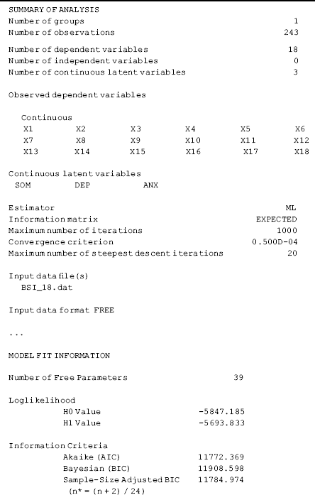
The first section of the Mplus output shown in Table 2.2 gives the summary of the analysis. It tells that this is a single group modeling with 18 observed variables and 3 latent variables/factors; the sample size is N = 243 after LISTWISE deletion; the estimator used is ML; and the model estimation was finished with 20 iterations.

The MODEL FIT INFORMATION section of Mplus output provides information about overall model fit. The χ ² statistics for the model being tested is χ ² = 306.702, df = 132 (P = 0.000), which reject the null hypothesis of a good fit. As discussed in Chapter 1, the model χ ² statistic is highly sensitive to sample size, and the significance of the test should not be a reason by itself to reject a model. Note, in Mplus output the χ ² Test of Model Fit for the Baseline Model χ ² = 2250.622, df = 153 (P < 0.001) is much larger than the χ ² Test of Model Fit χ ² = 306.702, df = 132 (P < 0.001). The Baseline Model in Mplus is similar to, but a little different from, the Independence Model defined in other SEM computer programs like LISREL. Suppose y represents dependent variables and x represents independent variables, the Independence Model is defined in LISREL with Cov(y, y) = 0, Cov(y, x) = 0, and Cov(x, x) = 0; in contrast, Cov(y, y) = 0, Cov(y, x) = 0, but Cov(x, x) ≠ 0 are defined for the Baseline Model in Mplus.

For a CFA, the baseline model is defined as a model in which all factor loadings are set to 1, and all variances/covariances of the latent variables/factors are set to 0, and only the intercepts and residual variances of the observed indicators (dependent variables in CFA) are estimated. For example, if we specify our example CFA as the following:

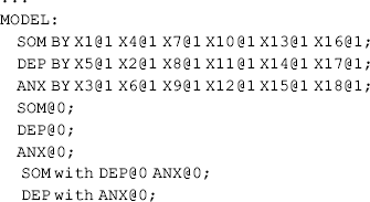
Then the estimated χ ² statistic of the target model will be identical to that of the baseline model (χ ² = 2250.622, df = 153, P < 0.001).

In regard to model fit, Table 2.2 shows that both CFI = 0.917 and TLI = 0.903 are ≥ 0.90, indicating an acceptable fit. The estimated value of RMSEA (0.074) is within the range of fair fit (0.05– 0.08). However, the upper limit of its 90% CI (0.063, 0.085) is outside the boundary (i.e., > 0.08), and the close fit test (P = 0.000) shows a rejection of the close fit (i.e., RMSEA ≤ 0.05). Yet, SRMR (= 0.052) is less than 0.08, indicating a good fit. As both CFI and TLI are greater than 0.90, and both RMSEA and SRMR are less than 0.08, overall, the model fit is acceptable.

Table 2.2 Selected Mplus output: three- factor CFA in analysis of COVS.

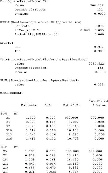
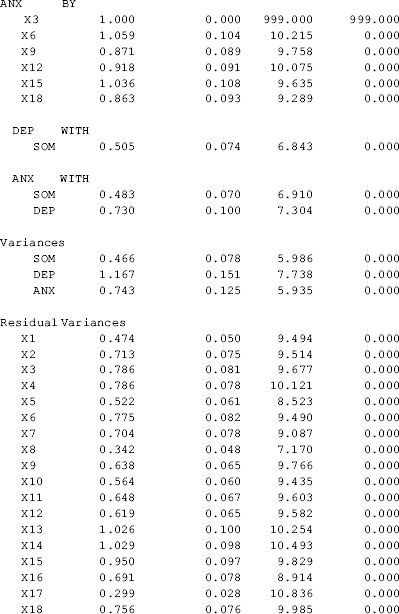
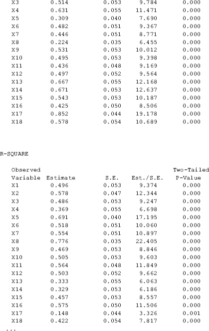
In the Model Results section of Mplus output, the estimated factor loadings, variances and covariances of the latent variables, as well as residual variances, appear along with their standard errors, t- ratios, and P- values.

Traditionally, CFA is estimated based on analysis of COVS. The covariance matrix is computed from deviation scores so that the means of all observed indicators are zero. As a result, item intercepts and factor means are excluded from model estimation. Since version 5, Mplus estimates models based on analysis of MACS. In a single group model, factor means are all set to zero by default for the purpose of model identification, while item intercepts are estimated.

The standardized parameter estimates are reported in the STANDARDIZED MODEL RESULTS section of the output. The STDYX Standardization in Mplus is equivalent to the complete standardized estimates provided by LISREL and other SEM programs.

All the indicators, except x₁₇, have a factor loading greater than 0.40, thus meeting the traditional cut- off point of factor loadings. The indicator x₁₇ has a lower standardized factor loading (0.38), suggesting that it is a weaker indicator of the latent factor DEP. However, its factor loading is statistically significant, thus we would like to keep this indicator in the model.

Model estimated item reliability. The estimated R- square (squared standardized factor loading) or squared multiple correlations of the items provide information on how much variance of each observed variable is accounted for by the factor(s) that it is loaded on. For example, indicator x₁ has a standardized factor loading of 0.704, then its R- square value or the squared multiple correlation is 0.704² = 0.496. Recall, the squared multiple correlation estimated from the CFA model is a measure of strength of a linear relation between an indicator and its underlying factor, representing how much variance of the indicator is explained by the underlying factor. It is also considered as a model estimated item reliability. In this example, x₈ has the highest R- square (0.78), while x₁₇ has the lowest (0.15).

Model estimated scale reliability: The scale reliabilities can be estimated using Equation (2.4). For example, the scale reliability for factor SON can be calculated as:

The scale reliabilities for subscales DEP and ANX can be calculated similarly. We leave the calculations as an exercise for readers.

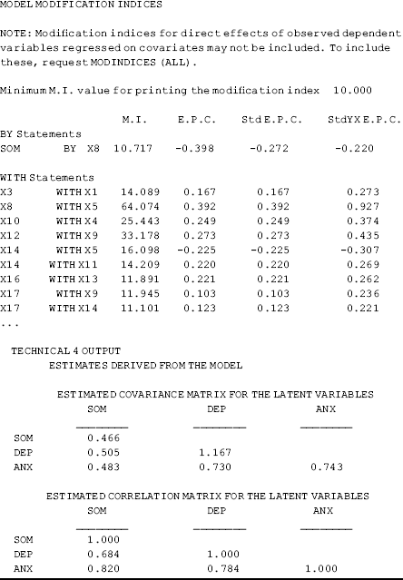
The correlations between the latent variables can be requested in Mplus output by using option TECHNICAL4 in the OUTPUT command. In this example, the correlations between SOM, DEP, and ANX are high ranging from 0.68 to 0.82.

The option MOD in the OUTPUT command requests model MIs and the associated EPC for fixed parameters specified in the model. By default, Mplus prints out the MI that is 10.0 or greater. A high MI value indicates that the corresponding fixed parameter could be freed to improve model fit. In our example model, nine error covariances have MI value greater than 10.0, and the covariance () between errors associated with indicators x₅ and x₈ has the highest MI value (64.074), indicating that freeing this parameter would reduce the model χ ² statistic by 64.074.

Respecifying the model based on MIs. We first free the parameter that has the largest MI value (64.1) by specifying a statement ‘ X5 WITH X8; ’ on the MODEL command line. As a result, model fit was substantially improved: CFI = 0.941, TLI = 0.932, RMSEA = 0.062, RMSEA 90% CI (0.051, 0.074), and SRMR = 0.045. However, the close fit test (P = 0.042) still rejects the null hypothesis of RMSEA ≤ 0.05. We then further freed the error covariance () associated with indicators x₉ and x₁₂, which had a MI value of 33.624 after was set free. The two error covariances are set free in the following Mplus program.

Mplus Program 2.2

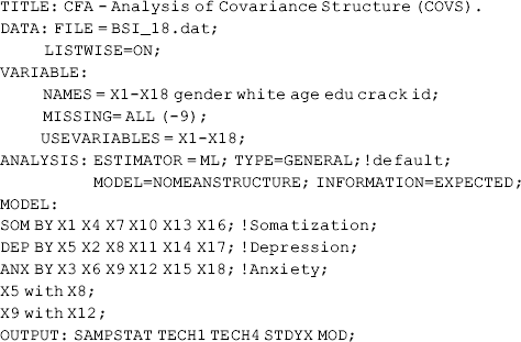
where the statements X5 with X8 and X9 with X12 set the two error covariances ( and ) as free parameters in model estimation. After these two error covariances were freed, factor loading estimates remain unchanged, but all the fit indices have been improved with higher CFI and TLI, smaller AIC, BIC, and ABIC, as well as smaller RMSEA and SRMR. In addition, the P- value close fit test increased to P = 0.297, indicating the model fits data much better.

As aforementioned, correlated measurement errors in a CFA model suggest that the associated indicators also measure something else in common in addition to the latent construct they are designed to measure. If we want to specify error terms to be correlated, the correlation must be substantively justified. It appears that the correlated item errors in our example are due to similar wording in the corresponding questions of the BSI- 18 instrument (see Appendix 2.A).

Analysis of MACS. Mplus Programs 2.1 and 2.2 estimate the model based on the traditional analysis of COVS where only the variance/covariance of the observed variables are analyzed in modeling. In other words, all variables in the model are measured as deviations from their means, and intercepts of regression equations and means of variables are irrelevant to the analysis. Most computer software/programs for SEM carry out SEM based on COVS by default.

When intercepts/thresholds and means are involved in model estimation, both the means and the variance/covariance structures of the observed variables need to be analyzed. Such an approach is called analysis of MACS in SEM. Starting with version 5, Mplus implements model estimation based on analysis of MACS by default. Hereafter in the book, all the models will be estimated based on MACS. The following Mplus program reruns the model based on MACS.

Mplus Program 2.3

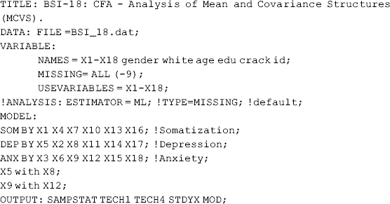
The model results of CFA based on analysis of MACS include intercept estimates of the observed indicators. The parameter estimates, such as factor loadings and variances of factors and residuals basically remain unchanged like those of CFA based on COVS.

Note that in Mplus Programs 2.1 and 2.2, where the model is estimated based on COVS, missing values can only be handled using traditional approaches, such as LISTWISE deletion or PAIRWISE deletion. The LISTWISE = ON statement in the DATA command was removed from the Mplus Program 2.3. Since Mplus version 5, the TYPE = MISSING option is the default in the ANALYSIS command to allow missing data in analysis using the expectation– maximization (EM) algorithm (Little and Rubin, 2002), assuming ignorable missing (i.e., MCAR or MAR). The FIML is implemented and every piece of information available in the data will be used for model estimation.¹⁰ To deal with missing data, the FIML is superior to other approaches, such as LISTWISE deletion, PAIRWISE deletion, and similar response pattern imputation (Enders and Bandalos, 2001). The model results suggest that with missing data modeling, the entire sample (N = 248) is used for data analysis, and model fit indices are somewhat improved.

Item parceling. In our example CFA model, there are 18 indicators/items (6 indicators/items per factor). As suggested by the modification indices (MIs) estimated by Mplus, our model will have a better fit when two error covariances are set free. Here we demonstrate item parceling using the item- pairs approach to make a more parsimonious model. With item- pairs parceling, the first two items of each factor are averaged to form the first item pair, the next two items are averaged to form the second pair, and so forth. Using item pairs has advantages over using the original individual items as the item- pairs tend to be more reliable, to be more normally distributed, and to have less idiosyncratic variance than do individual items. It is also justified by the small sample size, particularly for the multiple group analyses (Marsh and O' Neill, 1984; Hau and Marsh, 2004). The Mplus program follows.

Mplus Program 2.4

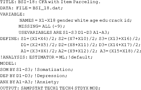
where item parcels S1– S3, D1– D3, and A1– A3 are created by averaging item pairs in each subscale of the BSI- 18 in the DEFINE command. These item parcels are then used as new indicators of the three latent variables/factors (i.e., SOM, DEP, and ANX). This parsimonious model fits data very well without having to specify any error covariance.

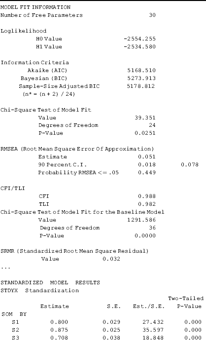
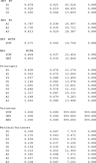
Table 2.3 shows that the model goodness- of- fit has been substantially improved. The model χ ² statistic, log- likelihood function, and information criteria indices are much smaller. Both CFI and TLI are above 0.95; SRMR = 0.032; RMSEA = 0.051, with a 90 % CI of (0.018, 0.078); and the close fit test is not statistically significant (P = 0.449), indicating that the close test hypothesis (i.e., RMSEA ≤ 0.05) cannot be rejected. The model fits data very well without specifying any measurement error covariance. This example shows that item parceling is a useful approach to develop a more parsimonious model and improve model fit without losing information. Readers are encouraged to try item parceling with different methods introduced in Section 2.1.

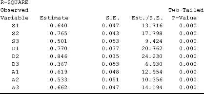
Table 2.3 Selected Mplus output: three- factor CFA using item- pairs parceling.