5.3 Multi-Group LGM

In applications of LGMs discussed in Chapter 4 it is assumed that individuals are randomly sampled from a single target population. In many cases, however, researchers encounter the fact that individuals can be identified as belonging to different populations (e.g., rural drug users in Ohio vs. Kentucky in our example) or groups (e.g., intervention vs. control groups) in their studies. To study differences in outcome growth trajectory over time between different known populations/groups, the LGM can be extended to multi-group LGM where the same LGM will be implemented simultaneously for each of the populations/groups. The estimated latent growth factors (i.e., latent growth intercept and slope factors) that determine the outcome growth trajectory may vary by population/group. Invariance of the growth trajectory across populations/groups can be tested in multi-group LGM.

The data (data file 2_Site_Longitudinal.dat) used for demonstration of multi-group LGMs are also selected from the samples of the rural drug user studies in Ohio and Kentucky (Wang et al., 2007). The data set 2_Site_Longitudinal.dat were collected from four interviews (baseline, 6-month, 12-month, and 18-month after baseline) in the two studies. The outcome measures (i.e., y₁ − y₄) are crack-cocaine use frequency in the past 6 months prior to each interview, which was measured on a seven-point scale from 0 (no use), 1 (less than 4 times per month), 2 (about once a week), 3 (about 2–6 times a week), 4 (about once a day almost every day), 5 (about 2–3 times a day almost every day), and 6 (about 4 or more times a day almost every day). In this example we examine and compare growth trajectories of crack-cocaine use over a period of 18 months among rural drug users in Ohio and Kentucky. In the following Mplus program, a two-group LGM model is used to estimate the growth trajectories of crack-cocaine use in Ohio and Kentucky, respectively, without restrictions on the growth parameters across group.

Mplus Program 5.22

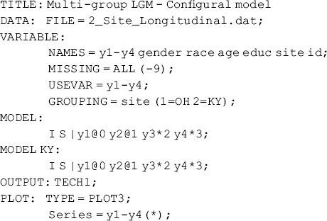
The above Mplus program specifies an unconditional LGM with free time scores for each of the two groups. I and S represent the latent intercept and slope growth factors, respectively, and they are estimated for each of the two samples simultaneously. The factor loadings for the latent intercept growth factors are set to 1.0 for each time point by default; time scores are set to 0 and 1.0 for the first and second time points, respectively, for the purpose of model identification; and free for the rest of the time points. As such, the growth trajectories will be determined by data, instead of the predefined functions (e.g., assumed linear or quadratic functions). The PLOT command at the end of the Mplus program produces graphs of outcome growth trajectories over time.

Table 5.17 shows that the model fits data very well (χ² = 8.346, df = 6, P = 0.214; RMSEA = 0.041, 90% CI = (0.000, 0.100); close-fit test P = 0.529; CFI = 0.996; TFL = 0.992; SRMR = 0.023). The model result show that Ohio and Kentucky rural drug users experienced different growth trajectory during the 18-month observation period. The observed and model estimated outcome growth trajectories are plotted in Figure 5.5 by sample.

Figure 5.5 Growth trajectories of crack-cocaine use by group.

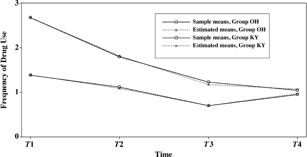
Table 5.17 Selected Mplus output: multi-group configural LGM.

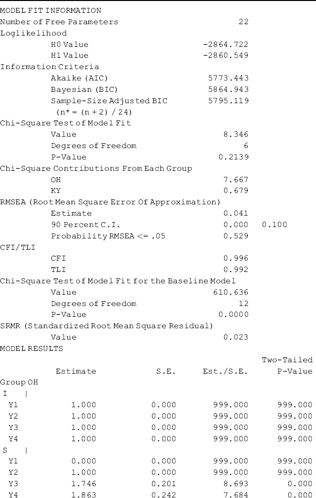
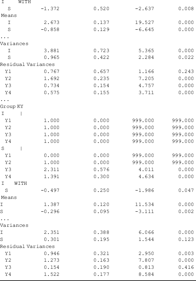
Figure 5.5 and Table 5.17 show some interesting findings. First, the initial level of crack-cocaine use was much higher in Ohio (I = 2.673, P < 0.001) than that in Kentucky (I = 1.387, P < 0.001). Secondly, the rate of decline in crack-cocaine use was faster in Ohio (S = −0.858, P < 0.001) than that in Kentucky (S = −0.296, P < 0.001). Thirdly, the covariance between initial level and rate of outcome change was negative and statistically significant in both states. It seems that rural drug users with higher initial level of crack-cocaine use reported larger decline in crack-cocaine use after baseline. However, such a relationship was much stronger in Ohio [Cov(I, S) = −1.372, P = 0.008] and in Kentucky [Cov (I, S) = −0.497, P = 0.047]. Fourthly, the growth trajectories were nonlinear in both populations. The level and change of crack-cocaine use over time in Ohio and Kentucky are estimated and shown in Table 5.18. Fifthly, the variances of the latent growth factors I and S seem noninvariant across samples: Var (I) = 3.881 (P = 0.000) and Var (S) = 0.965 (P = 0.022) for Ohio; Var (I) = 2.351 (P = 0.000) and Var (S) = 0.301 (P = 0.123) for Kentucky. And finally, the error/residual variances also seem noninvariant across the two samples. In the following, our analyses will focus on testing invariance of growth function; invariance of means, variances, and covariances of latent growth factors across samples.

Table 5.18 Model estimated outcome level and change over time by sample.

Test invariance of growth function: As discussed in Chapter 4, time scores or factor loadings of the latent slope growth factor determine growth function in a LGM. In Mplus Program 5.22 free time scores are specified to let the growth function be determined by data and the results of the model show different growth functions across groups (Table 5.17 and Figure 5.5). In the following Mplus program we will impose equality restriction on the time scores across groups. If the model χ² statistic change is statistically significant, compared with that estimated from Mplus Program 5.22, then we conclude the growth function significantly differs across groups.

Mplus Program 5.23

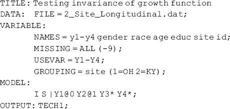
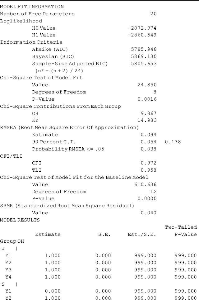
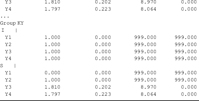
where the LGM model is only specified in the overall model. By default, time scores are held equal, thus growth function is held equal, across groups. Even though group specific MODEL commands are not specified in the Mplus program, the parameters (e.g., means, variances, and covariances) of the latent growth factors, as well as residual variances, are estimated by group without equality restrictions. For the purpose of model identification, the intercepts of the observed outcomes (y₁ − y₄) are all set to zero by default.

By comparing the results shown in Tables 5.17 and 5.19, we can see that equality restriction on the growth function resulted in a worse model fit: model χ² statistic increased from 8.346 to 24.850, and CFI reduced from 0.996 to 0.972. The change in χ² statistic is statistically significant ( = 16.504, df = 2, P < 0.001), and the change of CFI ( = 0.024) is greater than the cut-off point (0.01). Thus, we conclude that the outcome growth function is noninvariant across groups.

Table 5.19 Selected Mplus output: testing invariance of growth function.

Test invariance of latent growth factor means: In LGM the growth factors (e.g., I and S in this example) are latent variables, though they are not latent constructs in the sense of CFA. Instead, the observed outcome measures (y₁ − y₄ in this example) are used to construct the growth factors to represent the shape of individual growth trajectories, and the time scores are considered as the factor loadings of the latent slope factor. Testing invariance of means of the latent growth factors is in fact to test whether the average initial outcome level (i.e., the mean value of the latent intercept growth factor I) and average rate of outcome change (i.e., the mean value of the latent slope growth factor S) are invariant across groups. In this section, we will test invariance of the means of the latent intercept growth factor, latent slope growth factor, and both simultaneously across groups. The following Mplus program is to test invariance of the mean of the latent intercept growth factor (i.e., the mean of the initial outcome level at the baseline).

Mplus Program 5.24

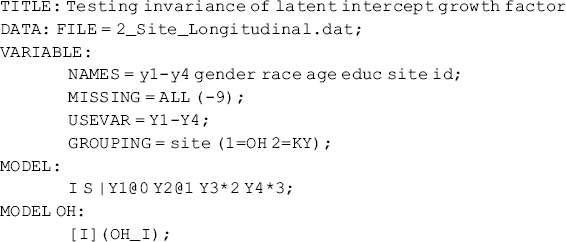
where the means of the latent intercept growth factors are labeled OH_I and KY_I for the Ohio and Kentucky samples, respectively. The MODEL TEST command is used to test the hypothesis of OH_I=KY_I. The resulting Wald test = 48.794 (df = 1, P < 0.001) indicates that the mean of the initial level of crack-cocaine use frequency among rural drug users in Ohio differed significantly from that in Kentucky.

The following Mplus program is to test invariance of the mean of the latent slope growth factor (i.e., the average rate of outcome change over time).

Mplus Program 5.25

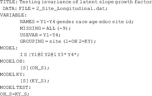
where the means of the latent slope growth factors are labeled OH_S and KY_S for the Ohio and Kentucky samples, respectively. The MODEL TEST command is used to test the hypothesis of OH_S=KY_S. The model results show a Wald test = 20.141, df = 1, P <0.001, indicating that the rate of outcome change over time is different on average between Ohio and Kentucky.

The following Mplus program is to test invariance of the means of both latent intercept and slope factors across groups.

Mplus Program 5.26

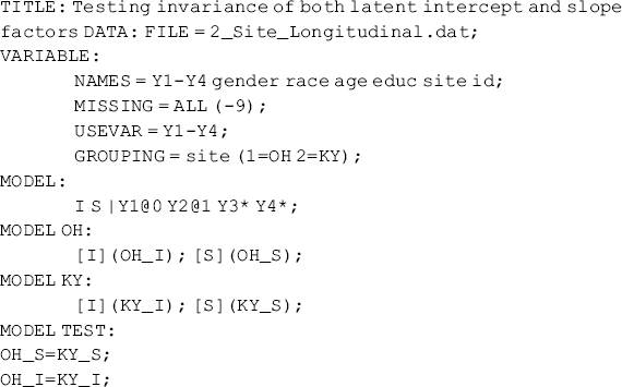
where invariance of the means of both latent intercept and slope growth factors are tested simultaneously in the MODEL TEST command. The resulting Wald test = 48.915, df = 2, P <0.001 is statistically significant, indicating that the two latent growth factors are noninvariant across groups. In other words, both the initial level of crack-cocaine use frequency at the baseline and the rate of change in crack-cocaine use over time were significantly different between Ohio and Kentucky rural drug using populations.

Using the same method, invariance of growth factor variances/covariances and residual variances can be readily tested. We will leave these tests to the interested readers for practice.

This chapter expands applications of SEM from single population/group to multiple populations/groups. We have discussed and demonstrated that invariance of measurement parameters (e.g., item intercepts, factor loadings, error variances) and noninvariance of structural parameters (e.g., factor variances/covariance, factor means, patch coefficients) across different populations/groups can be tested using multi-group modeling. A few issues need to be pointed out here. First, when applied to multiple samples from the same population, multi-group modeling is known as cross-validation modeling. If sample size is large enough, the sample under study can be randomly split into two subsamples where the first half sample is called the calibration sample, and the second half is the validation sample. The across-validation strategy is to test whether model estimates from the calibration sample can replicate over the validation sample (Byrne, 2006). The across-validation index, which is developed to measure across-validation by examining the discrepancy of the variance/covariance matrix between the calibration and validation samples (Cudeck and Browne, 1983; Browne and Cudeck, 1989), can be used to determine whether a model is replicable across calibration and validation samples. However, the multi-group SEM approach can be readily used to assess across-validation. Secondly, when the observed number of groups is large, and the group size (i.e., the number of cases per group) is small, multi-group modeling is not appropriate, instead, the MIMIC model discussed in Chapter 3, in which a grouping variable is included in the model as a predictor, can be used to test population heterogeneity in regard to factor means, as well as differential item functioning, although it does not allow to test invariance of factor loadings or factor variances/covariance. And finally, measurement invariance is relevant in longitudinal studies when a scale is administered over repeated occasions to the same sample of people. Note that multi-group CFA is not appropriate for testing measurement invariance across time because observations are not independent. Instead, a multiwave CFA model may be applied. In such a case, all observed indicator variables at different time points are included in the same model, in which error correlations between the same indicators across time are specified; each CFA factor at a later time point (e.g., time 2) is specified as an endogenous latent variable, and its corresponding factor at an earlier time point (e.g., time 1) is specified as an exogenous latent variable. The stability for the latent variables is measured by the standardized path coefficient linking these latent variables, controlling for measurement errors (Bagozzi and Edwards, 1998).

The multi-group models discussed in the chapter deal with population heterogeneity when a finite number of subpopulations/groups in a target population are known or observed. In the next chapter, we will discuss mixture models that are designed to handle population heterogeneity when a finite number of subpopulations/groups are a priori unknown.

Notes

1. For example, a few cross-loadings may be included in one group, but not in other groups; and a few different error covariances may be specified in different groups (Byrne, 1998).

2. In our example there is a common error covariance [i.e., Cov()] specified in the Ohio and Kentucky models, a group-specific error covariance [i.e., Cov()] in the Ohio baseline model, and two group-specific error covariances [i.e., Cov() and Cov()] in the Kentucky baseline model. This discrepancy in model specification should not affect model comparisons in regard to testing invariance in other parameters (Byrne, 1998).

3. The absolute values of the factor means cannot be estimated in multi-group CFA. The vector in Equation (5.2) actually represents factor mean differences between specific comparison groups and the reference group for which factor means are set to 0.

4. If the two samples were stored in two separate data sets (e.g., Ohio_data.dat and Kentucky_data_dat), two FILE statements are needed to read the two data sets simultaneously: ‘FILE(OH)= Ohio_data.dat;’ and ‘FILE(KY)= Kentucky_data_dat;’ where the labels ‘OH’ and ‘KY’ can be used in the group-specific MODEL commands.

5. The P-value of the LR χ² test can be calculated from the following SAS program: Data _null_; P_value=1-probchi(15.967, 15); Put P_value; Run;

6. in Equation (5.5) denotes error variances and covariances. Theoretically speaking, error covariances should be zeros although in practice some of them may be specified as free parameters in a measurement model.

7. It should be reminded that the second-order factor could be empirically under-identified if any correlation between the three first-order lower-order factors is close to zero. Empirical under-identification is possible although it does not happen very often. Thus, correlations between lower-order factors should always be checked before conducting a higher-order CFA model.

8. By default, Mplus sets the factor loading of the first indicator (SOM in this example) to 1.0. This restriction can be released by putting the symbol ‘∗’ after the indicator.

9. Note that the model fit statistics/indices of the second-order three-factor CFA models are identical to the first-order three-factor models (Table 5.3) as the second-order part of the model is just identified with three indicators (first-order factors).

10. An arbitrary letter ‘E’ in the parentheses sets equality restriction on the intercepts of the first-order factors DEP and ANX. In Mplus both numbers and letters can be used as ‘indices’ in the parentheses of equality restrictions.

11. MLMV is for continuous outcomes and WLSMV for categorical outcomes.