3.1 MIMIC Model

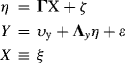
MIMIC model stands for multiple indicator multiple cause model, in which multiple indicators reflect the underlying latent variables/factors, and the multiple causes (observed predictors) affect latent variables/factors. When covariance structure (COVS) is analyzed, the MIMIC model is described as (Instead of assuming only one latent variable in a MIMIC model (Bollen, 1989), we assume one measurement model with one or more latent variables in a MIMIC model):

(3.1)

where multiple endogenous indicators ys are used to measure the endogenous latent variables s; no causal effects, but the covariance/correlations, are specified among the s because all latent variables are in one measurement CFA model; and s are affected by observed predictors xs, which are assumed to be perfect measures of the exogenous latent variables s (e.g., respondent self-reported gender status is often treated as a measure of his/her sex identity without measurement error).

When the MACS is analyzed, the MIMIC model is described as:

(3.2)

where is the vector of intercepts of indicators ys. Notice that there are no factor intercepts in Equation (3.2) because factor means/intercepts in a single group model must be set to zero for the purpose of model identification. Factor mean differences between groups can be examined in multi-group modeling that will be discussed in Chapter 5. The symbol ‘’ specifies identity between X and , which is obtained by fixing factor loadings to 1.0 (i.e., = 1) and measurement errors to 0 (i.e., = 0).

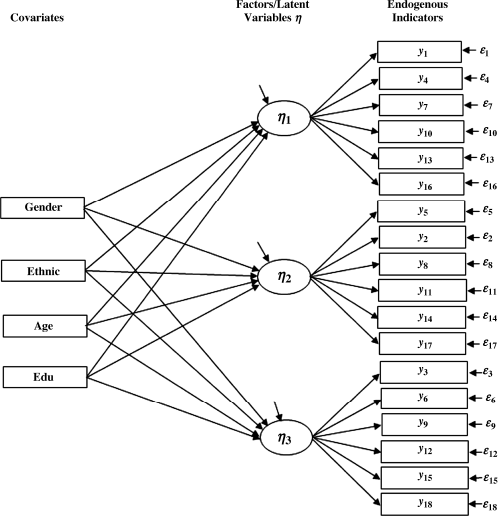
In this section, we illustrate a MIMIC model using the same BSI-18 data set that was partially used for models in Chapter 2. The MIMIC model specified in Figure 3.1 consists of two parts: (1) measurement model, in which 18 observed indicators/items measure three underlying latent variables/factors [i.e., SOM, somatization (); DEP, depression (); and ANX, anxiety ()] as discussed in Chapter 2; and (2) structural equations, in which observed x variables, such as gender (Gender:1, male; 0, female), ethnicity (Ethnic: 1, white; 0, non-white), age (Age), and education (Edu: 1, no formal education; 2, less than high school education; 3, some high school education; 4, high school graduate; 5, some college; and 6, college graduate) predict the three latent variables/factors.

Figure 3.1 MIMIC model.

The measurement part of the MIMIC model can be described as:

(3.3)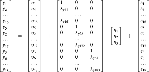

This is equivalent to

(3.4)

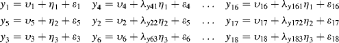
The measurement part of the MIMIC model has been already tested in the CFA models in Chapter 2. The new component in the MIMIC model is the structural equations that examine the causal relationships between the demographic variables and the latent variables.

The structural equation part of the MIMIC model can be specified in matrix notation:¹

(3.5)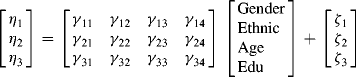

This is equivalent to

(3.6)

where the three multiple regression equations look like the simultaneous equation models in econometrics, in which multiple dependent variables are functions of a set of explanatory variables or predictors and the residual terms (i.e., , , ) of the equations are allowed to be correlated with each other. However, different from the traditional simultaneous equation models, the dependent variables in the MIMIC models are unobserved latent variables. This approach is clearly better than the traditional simultaneous equation models or multivariate analysis of variance (MANOVA) that assumes variables have no measurement errors.

The following Mplus program is to run the MIMIC model.

Mplus Program 3.1

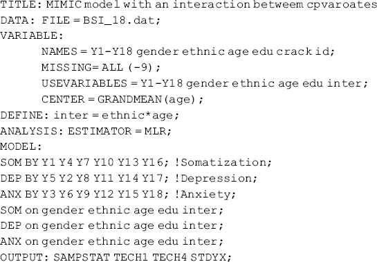
where data are read from data set BSI_18.dat. The observed variables y₁–y₁₈ are indicators of three latent variables (, SOM; , DEP; and , ANX), and four observed variables (Gender, Ethnic, Age, and Edu) are used to predict the latent variables. Considering the possible multivariate non-normality in the measures, the robust estimator MLR is used for model estimation.

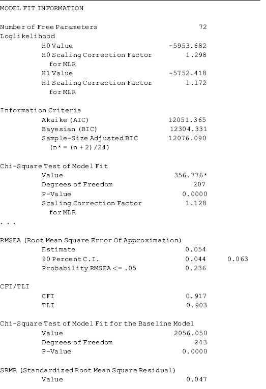
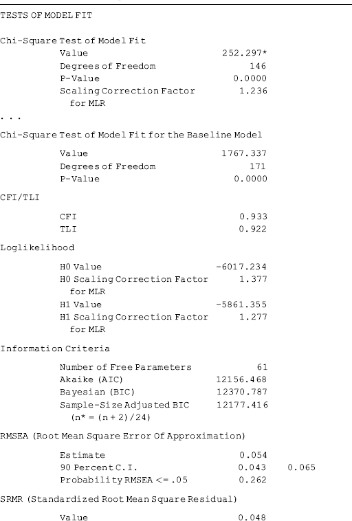
The results show that the model fits data very well: RMSEA = 0.055 (90% CI: 0.045, 0.064), close-fit test P = 0.207, CFI = 0.918, TLI = 0.904, and SRMR = 0.048 (Table 3.1).

Table 3.1 Selected Mplus output: MIMIC model.

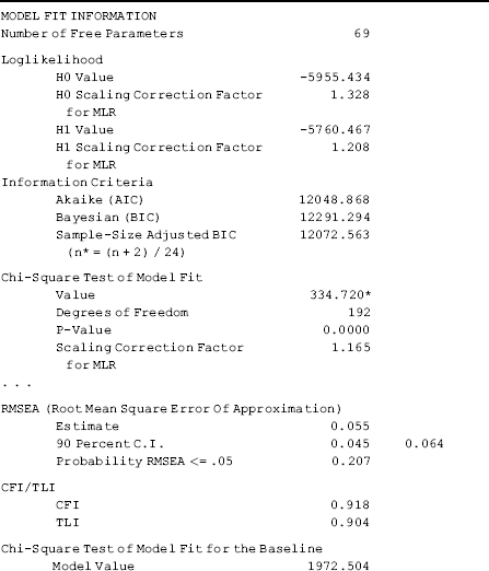
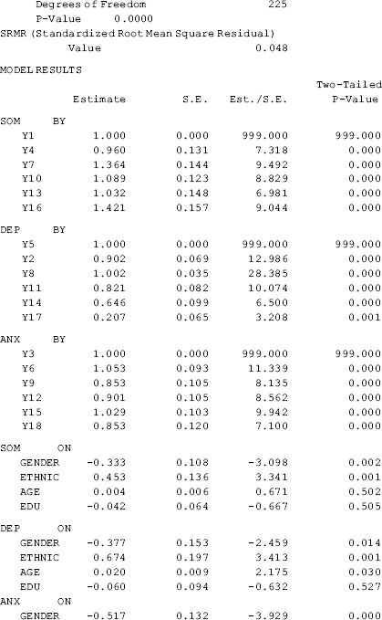
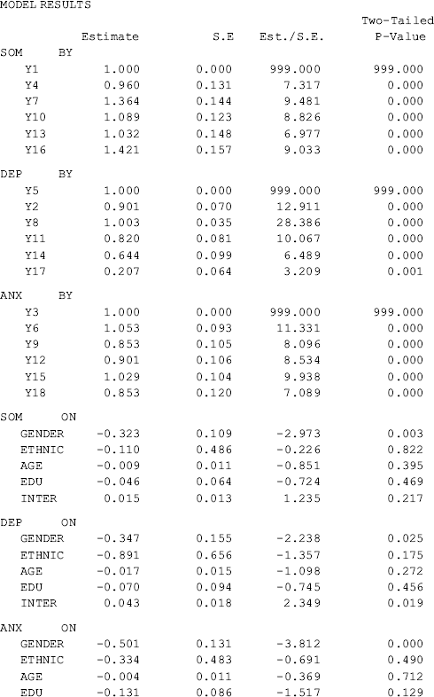
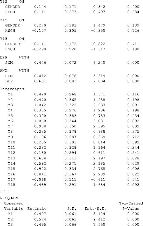
As the measurement model of the BSI-18 was well established in CFA modeling in Chapter 2, the estimated factor loadings basically remain unchanged in the MIMIC model. Gender has a significant negative effect (−0.377, P = 0.014), while both Ethnic (0.674, P = 0.001) and Age (0.020, P = 0.030) have a significant positive effect, on depression (DEP). The effect of Edu (−0.060, P = 0.527) on DEP is negative, but not statistically significant. Similar results are found for anxiety (ANX) and somatization (SOM), except that the effect of Age (0.004, P = 0.502) on SOM is not statistically significant.

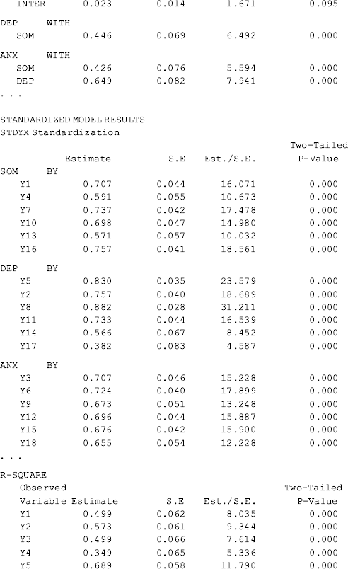
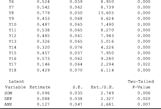
The estimated R² values for both the observed variables and the latent variables are provided by Mplus when the STDYX option is specified in the OUTPUT command. The explained variances in the latent variables SOM, DEP, and ANX vary from 0.07 to 0.12.

The variances of residuals , and in Equation (3.4) are model parameters 64, 66, and 69, and their covariances are parameters 65, 67, and 68 (see the PSI matrix in the TECHNICAL 1 OUTPUT section of Table 3.1). These parameters are elements of model parameter matrix Ψ (Table 1.2). Option TECH4 specified in the OUTPUT command provides estimated variance/covariance matrix for the latent variables, as well as correlations between the latent variables.

Attention needs to be paid to interpretation of some parameter estimates reported in the Mplus output. First, as the observed predictors (x variables) are treated as perfect measures (e.g., Gender is a measure of respondent's sex identity without measurement error), they are considered as exogenous ‘latent’ variables s. As a result, their variances, covariances, and correlations are reported in the TECHNICAL 4 OUTPUT. Secondly, when covariates are included, the covariances between the endogenous factors reported in the MODEL RESULTS section of Mplus output are in fact estimated residual covariances. For example, the covariance between DEP and SOM (0.453, P < 0.001) in the MODEL RESULTS section is actually covariance between residuals and ; and the estimated covariance (0.507) and correlation (0.685) between factors DEP and SOM are reported in the TECHNICAL 4 OUTPUT. Finally, when MACS is analyzed in a single group model in Mplus, factor means/intercepts are fixed to zero by default. However, estimated nonzero factor ‘means’ are reported in TECHNICAL 4 OUTPUT for the example MIMIC model (Table 3.1). This is because covariates are involved in the model and the factors take information about the covariates into account. Once we remove the covariates from the model, the factor means/intercepts reported in TECHNICAL 4 OUTPUT would become zero.

Interaction effects between covariates. In multiple regression models, it is a common practice to examine interaction effect of explanatory variables. For example, in a multiple linear regression y = a + b₁x₁ + b₂x₂ + e, the two explanatory variables x₁ and x₂ may have an interaction effect on the dependent variable y. The interaction term can be created by multiplying the two variables (e.g., x₁^∗x₂), leading to y = a + b₁x₁ + b₂x₂ + b₃x₁∗x₂ + e. Thus, the interaction effect b₃ implies that the effect of x₁ (x₂) on the dependent variable depends on the value of x₂ (x₁).

Two points are important with respect to the interactions (Hox, 2002). First, if an interaction effect is statistically significant, the corresponding main effects must remain in the model, no matter whether they are statistically significant or not. Secondly, variables involved in an interaction must have meaningful 0 values in their observed measures. Otherwise, the main effect of the counterpart variable will not be meaningful. Suppose there is an interaction between x₁ and x₂, the main effect of x₁ is interpreted as the effect of x₁, corresponding to a 0 value of variable x₂. If variable x₂ does not have a meaningful 0 value in the sample under study, then the main effect of x₁ is not meaningful. To avoid such inappropriate interpretation of main effects, the variables involved in interactions should be centered from the sample mean (i.e., measured as deviations from the sample means) (Hox, 1994). In addition, to minimize the potentially confounding effects of multicollinearity, the variables involved in an interaction may be further standardized with mean of 0 and standard deviation of 1.0 before constructing the product terms (Marsh, Tracey, and Craven, 2006).

Mplus Program 3.2 carries out a MIMIC model with an interaction effect between covariates Age and Ethnic.

Mplus Program 3.2

As the variable Age does not have a meaningful 0 value in the current sample, this variable is grand-mean centered using the CENTER = GRANDMEAN statement in the VARIABLE command. The interaction (Inter) between Age and Ethnic was created in the DEFINE command. Note that in the USEVARIABLES statement, all new variables (e.g., Inter in this example) created from the DEFINE command variables must be placed after the variables that are listed in the NAMES statement in the VARIABLE command; otherwise, Mplus will show an error message.

Table 3.2 shows that the model fits data very well. The interaction between Age and Ethnic on depression (DEP) is statistically significant (0.043, P = 0.019); thus, interpretation of the effect of covariate Age on DEP must take into consideration both its main effect and the interaction effect no matter whether its main effect is statistically significant or not. The same applied to the effect of covariate Ethnic.

Table 3.2 Selected Mplus output: MIMIC model with covariate interaction.

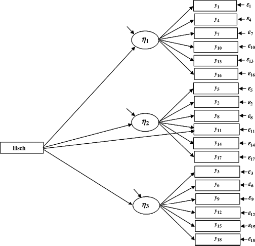
Differential item functioning (DIF). In a MIMIC model, we can not only investigate the effect of a covariate on factors, but also investigate whether the covariate directly affects the observed endogenous indicators (Muthén, 1989). A significant direct effect of a covariate on an observed indicator variable indicates that the value of the indicator variable differs by the values of the covariate, holding the latent variable/factor constant. Figure 3.2 shows a MIMIC model with a covariate (Hsch) (1, high school or above education; 0, less than high school) where the covariate affects all the three factors [i.e., SOM (), DEP (), and ANX ()], as well as one of the endogenous indicators y₁₁ (feeling worthless). A significant slope coefficient of regressing a factor (e.g., DEP) on the covariate Hsch indicates the difference in mean value of the factor between those with and without high school or above education. In contrast, a significant slope coefficient of regressing an indicator (e.g., y₁₁) on the covariate implies DIF; that is, the value of the item y₁₁ differs (or there exists a systematic difference in response to the item) between respondents with and without high school or above education, holding the latent variable constant (e.g., with the same level of depression). This kind of extended MIMIC model has been used to study DIF in measuring depression (Gallo, Anthony, Muthén, 1994; Grayson et al., 2000) and functional disability (Fleishman, Spector and Altman 2002). The following Mplus program runs the model specified in Figure 3.2.

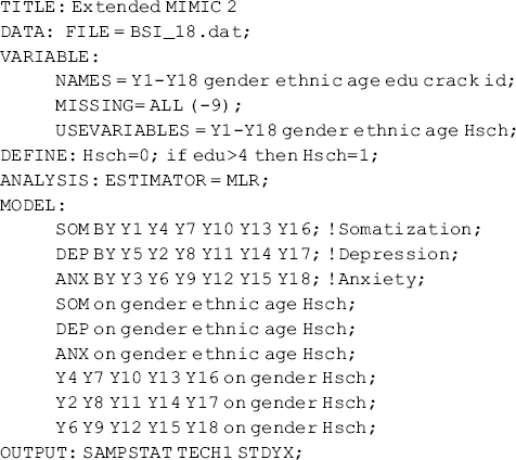
Figure 3.2 Differential item functioning in a MIMIC model.

Mplus Program 3.3

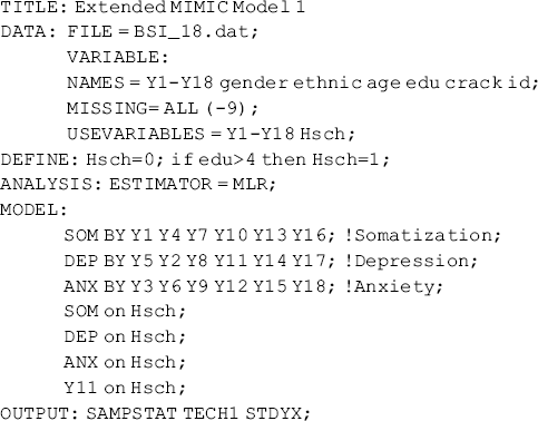
where we create a dummy variable Hsch (1, high school or above education; 0, less than high school education) in the DEFINE command. In the Mplus program, not only the factors SOM, DEP, and ANX, but also the observed endogenous indicator y₁₁, are regressed on covariate Hsch.

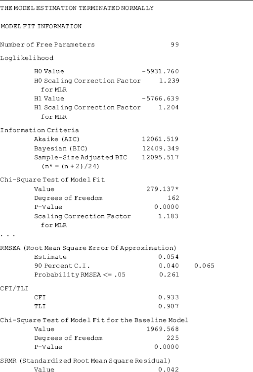
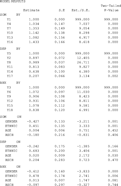
Table 3.3 shows that the covariate Hsch does not have significant effect on any of the three mental health factors (SOM, DEP, and ANX). This indicates invariance in the means of the factors between the two education achievement groups (i.e., high school or above vs. less than high school). However, Hsch has a significant negative effect (−0.636, P = 0.001) on the observed indicator variable y₁₁ (feeling worthless) of the depression factor (DEP). This implies that participants with less than high school education will score higher on the item y₁₁ than those with high school or above education, controlling for the factor of depression. In other words, higher educated people would be less likely to feel worthless, compared with the lower educated people, holding the level of the underlying factor of depression constant.

Table 3.3 Selected Mplus output: extended MIMIC model – 1.

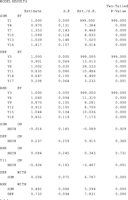
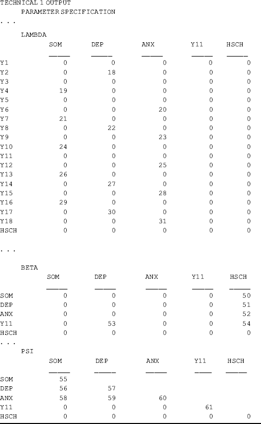
Traditionally, exogenous observed variables (e.g., Hsch in this example) are not allowed to predict endogenous indicators (e.g., y₁₁ in this example) in SEM, but this can be done easily in Mplus. When doing so in Mplus, factor loadings of the corresponding indicators are included into the BETA matrix (Muthén, 1989). From the section of TECHNICAL 1 OUTPUT in Table 3.3, we can see that the factor loadings of indicator y₁₁ are not reported in the LAMBDA parameter matrix, but in the BETA matrix (parameter 53); accordingly, the variance of indicator y₁₁ (parameter 61) is reported in the PSI parameter matrix (variance/covariance matrix of disturbance ζ).

The model specified in Figure 3.2 can be further extended to test DIF for all the indicators of each factor in the model as shown in the following Mplus program.

Mplus Program 3.4

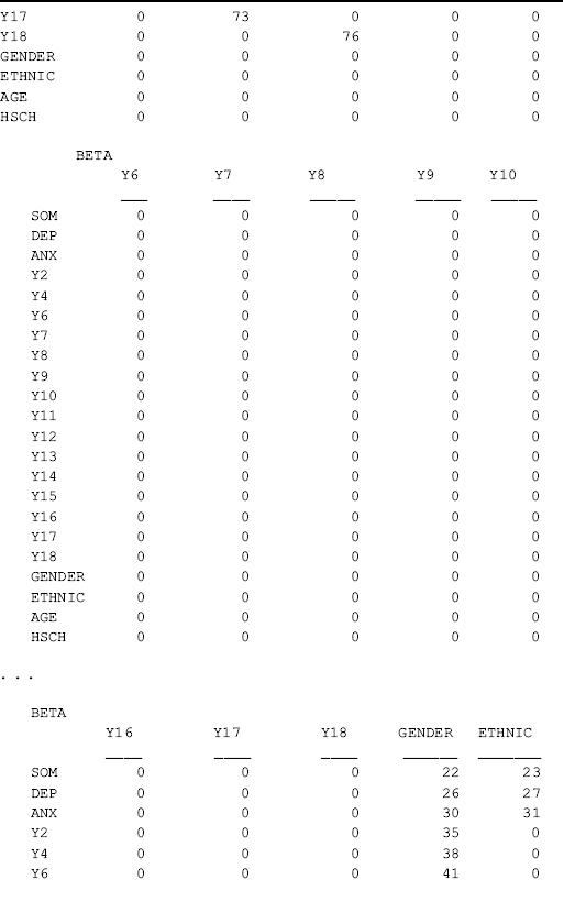
where the observed indicator variables are specified to load to the factors in the same way as in previous models; and all indicators, except one,² of each latent variable are regressed on two dichotomous covariates (Gender and Hsch). Note that in model estimation, all the factor loadings are included in the BETA matrix, instead of in the LAMBDA matrix. The slope coefficients of regressing indicators on covariates are included in the BETA matrix; and the variances/covariances of measurement errors are included in the PSI matrix, instead of in the THETA matrix (Muthén, 1989; Kaplan, 2000) (see the TECHNICAL 1 output in Table 3.4). However, the interpretations of these parameter estimates remain the same as in the previous CFA and MIMIC models.

Table 3.4 Selected Mplus output: extended MIMIC model – 2.

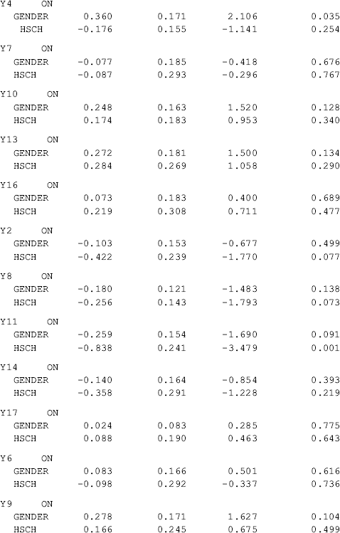
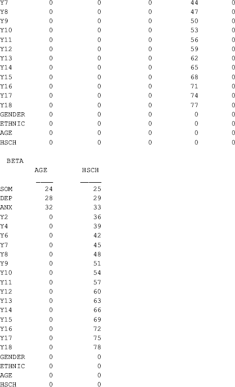
Among all the indicators, y₄ is significantly positively affected by Gender (0.360, P = 0.035), and y₁₁ is significantly negatively affected by Hsch (−0.838, P = 0.001). This indicates that there is no DIF for most of the BSI-18 items, except for the two items. The positive effect of Gender on y₄ (chest pains) indicates that male drug users would be more likely to report chest pains than females given the same level of somatization. In other words, there is significant gender difference in response to item y₄ (chest pains), controlling for the underlying factor SOM. Given the same level of depression, the significant negative effect of Hsch on y₁₁ (feeingl worthless) indicates that participants with higher education would be less likely to feel worthless, compared with those with lower education (i.e., less than high school), given the same level of depression.

Based on the effects of covariates on latent variables and endogenous indicator variables in a MIMIC model, one is able to: (1) test whether factor means are different between groups by examining the effects of covariates on factors; and (2) test whether responses to the same items differ between groups or whether DIF exists by examining the effects of covariates on items. For example, covariate Hsch has no effect on any of the three factors (SOM, DEP, and ANX) in the extended MIMIC model, indicating invariance in the factor means between the two education groups. However, the significant effect of Hsch on item y₁₁ indicates noninvariance in response to the item or the item displays DIF between these two education groups.

The extended MIMIC model can test both noninvariances in factor means and intercepts of indicators. However, unlike multi-group CFA that we will discuss in Chapter 5, the MIMIC model is unable to test noninvariance in factor loadings, factor variances/covariances, and measurement error variances/covariances. Multi-group CFA enables us to test noninvariance in all the measurement parameters and structural parameters. However, compared with the multi-group CFA model, the extended MIMIC model has some unique advantages. For example, it does not require a large sample size when the number of groups for comparison is large, thus the number of cases per group is small. In particular, when the grouping variable is a continuous measure (e.g., age), multi-group CFA is not appropriate, but the extended MIMIC model is.