4.3 Multi-Process LGM
In previous sections of this chapter, our modeling focuses only on a single outcome growth process. The LGM can be extended to simultaneously model multiple outcome growth processes, which could be either parallel or sequential (Muthén and Muthén, 1998–2010). In this section we will discuss and demonstrate parallel-process LGM. The following equations describe an unconditional parallel multi-process LGM:
where Equation (4.14) is referred to as the within subject model, in which ![]() is the ith observed outcome measures at time point tt for the mth outcome measure. Model parameters
is the ith observed outcome measures at time point tt for the mth outcome measure. Model parameters ![]() and
and ![]() are the latent intercept and slope growth factors for the mth outcome growth process. Equations (4.15) and (4.16) are referred to as between subject models for the mth outcome measure, in which
are the latent intercept and slope growth factors for the mth outcome growth process. Equations (4.15) and (4.16) are referred to as between subject models for the mth outcome measure, in which ![]() and
and ![]() serve as dependent variables,
serve as dependent variables, ![]() represents the estimated overall mean initial level of the outcome, and
represents the estimated overall mean initial level of the outcome, and ![]() is the average rate of outcome change, and
is the average rate of outcome change, and ![]() and
and ![]() are residuals.
are residuals.
In a conditional parallel multi-process LGM, covariates are added into Equations (4.15) and (4.16), then we have:
(4.17) ![]()
(4.18) ![]()
where a set of time-invariant covariates are included to predict the variation in the latent intercept and slope growth factors. Time-varying covariates can be readily added into Equation (4.14).
In this section we demonstrate a parallel process unconditional LGM, in which repeated measures of two outcomes are simultaneously modeled, assuming the two growth trajectories are associated with each other. LGM with more than two growth processes can be estimated in the same way if sample size is large enough. The more growth processes involved in a model, the bigger the sample size needed because more parameters need to be estimated.
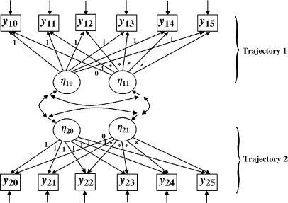
The unconditional parallel LGM with six time-point repeated measures is shown in Figure 4.10 where repeated measures of y10 − y15 (i.e., BDI-defined depression score) represent one growth process, while y20 − y25 (i.e., crack-cocaine use frequency) represent another growth process. The covariance between the latent intercept growth factors of the two growth trajectories would provide information about the association between the two outcomes at the beginning of the observation time period; the covariance between the latent slope growth factors would indicate how the rates of changes in the two outcomes were associated with each other. If a causal relationship between the outcomes under study can be theoretically defined, the causal effects can be tested in the model by replacing the covariances with path coefficients. Since the causal relationship between crack-cocaine use and depression disorder is complex and uncertain, associations rather than casual effects between the latent growth factors of the two outcome measures were specified in the model here. The corresponding Mplus program follows.
Figure 4.10 Unconditional parallel LGM.
Mplus Program 4.12
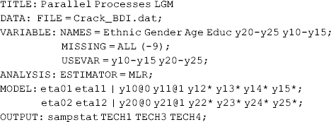
To be consistent with the notations used in Figure 4.10, measures of BDI score (y0 − y5) and crack-cocaine use frequency (z0 − z5) named in the previous Mplus programs are renamed as y10 − y15 and y20 − y25, respectively, in Mplus Program 4.12. Two LGMs with free time scores are specified in the MODEL command to simultaneously model the growth processes of BDI defined depression and frequency of crack-cocaine use among the drug users. The association (i.e., growth factor covariances) between the two growth processes will be estimated by default.
The estimated time scores ![]() and
and ![]() (see Table 4.13) for the two outcome growth trajectories are a departure from the linear time scores
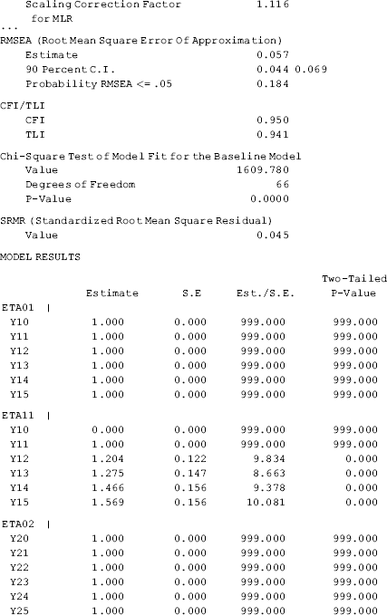
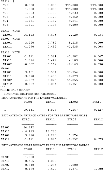
(see Table 4.13) for the two outcome growth trajectories are a departure from the linear time scores ![]() , thus we conclude that the two outcomes had all changed over time in a nonlinear way. The average initial level of BDI score was about eta01 = 19.13 (P < 0.001) at baseline, declined rapidly (eta11 = −3.878, P < 0.001) during the first 6-month period after the baseline, and then the decline leveled off. A similar pattern was found for another outcome (i.e., crack-cocaine use frequency) growth trajectory. The initial levels of the two outcomes were significantly positively correlated with each other: the covariance between y10i and y20i is Cov(eta02, eta01) = 3.92, P < 0.0001. The rate of change in the two outcomes was also significantly positively correlated [Cov(eta12, eta11) = 1.88, P < 0.0001]. This indicates that the level of BDI and crack-cocaine use frequency and the rates of change in the two outcome measures are positively related to each other although the directions of causal relationship between the outcomes were uncertain. In addition, the rate of change in each of the outcomes was significantly negatively correlated with its initial level; that is, the covariance between the latent intercept and slope growth factors in each growth process is negative and statistically significant [Cov(eta01, eta11) = −16.12, P = 0.034; Cov(eta02, eta12) = −0.352, P = 0.030], indicating that the higher the initial level, the smaller the rate of change in the outcome (Table 4.13). Since the rate of outcome change (i.e., the slope growth factor) is negative, the negative covariance indicates that those with higher initial outcome scores had a larger decline in the outcome.
, thus we conclude that the two outcomes had all changed over time in a nonlinear way. The average initial level of BDI score was about eta01 = 19.13 (P < 0.001) at baseline, declined rapidly (eta11 = −3.878, P < 0.001) during the first 6-month period after the baseline, and then the decline leveled off. A similar pattern was found for another outcome (i.e., crack-cocaine use frequency) growth trajectory. The initial levels of the two outcomes were significantly positively correlated with each other: the covariance between y10i and y20i is Cov(eta02, eta01) = 3.92, P < 0.0001. The rate of change in the two outcomes was also significantly positively correlated [Cov(eta12, eta11) = 1.88, P < 0.0001]. This indicates that the level of BDI and crack-cocaine use frequency and the rates of change in the two outcome measures are positively related to each other although the directions of causal relationship between the outcomes were uncertain. In addition, the rate of change in each of the outcomes was significantly negatively correlated with its initial level; that is, the covariance between the latent intercept and slope growth factors in each growth process is negative and statistically significant [Cov(eta01, eta11) = −16.12, P = 0.034; Cov(eta02, eta12) = −0.352, P = 0.030], indicating that the higher the initial level, the smaller the rate of change in the outcome (Table 4.13). Since the rate of outcome change (i.e., the slope growth factor) is negative, the negative covariance indicates that those with higher initial outcome scores had a larger decline in the outcome.
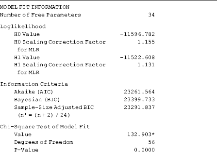
Table 4.13 Selected Mplus output: parallel-processes LGM.
If theory or empirical findings provide information about the directions of causal relationships between the growth factors (e.g., eta01 predicts eta11 or eta11 predicts eta12), causal relationships can be specified in the model. For example, suppose the initial level and rate of change in BDI scores were a function of crack-cocaine use frequency, the following Mplus program will estimate the causal relationships between the corresponding latent growth factors.
Mplus Program 4.13
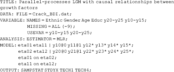
where the two ON statements in MODEL command specify the hypothesized causal relationships between the latent growth factors of the two growth processes. The model results (not reported here) show that the slope coefficient of regressing eta01 on eta02 is 2.303 (P < 0.0001); while the slope coefficient of regressing eta11 on eta12 is 2.946 (P < 0.0001).
