4.2 Nonlinear LGM

When outcome change over time occurs in a nonlinear fashion, nonlinear growth models should be considered. The LGM allows for the flexibility of factor loadings being associated with the slope growth factor to fit various nonlinear growth trajectories. The commonly used approaches to specify nonlinear growth trajectory include, but arenot limited to, polynomial function, orthogonal polynomial function, piecewise polynomials, and free time scores.

A polynomial function is often used to specify nonlinear outcome change. A polynomial time function can be constructed by introducing quadratic, cubic, or higher order functions of time scores. The order of the polynomial function to choose depends on patterns of change in the outcome over time. Theoretically, the orders of polynomial function can go as high as (T − 1) where T is the total number of observation time points. However, the higher the polynomial order, the more difficult it is for the model to fit and the more difficult it is to interpret the results. Here our examples were confined to a quadratic function (i.e., the second order of the polynomial time function) even though higher polynomial terms might be justified in some instances. A quadratic growth means one departure (either curve up or curve down) from linearity. With the regular quadratic change assumption, an additional latent slope growth factor with appropriate time scores can be added to represent the quadratic term (Muthén and Muthén, 1998–2010).

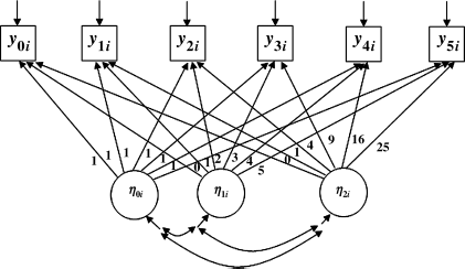
Figure 4.5 shows an unconditional quadratic LGM that includes three latent growth factors: , the intercept growth factor; , the linear slope growth factor; and , the quadratic slope growth factor. The time scores (i.e., 0, 1, 4, 9, 16, 25) for the quadratic slope factor are the squared values of the linear time scores (i.e., 0, 1, 2, 3, 4, 5). The quadratic slope growth factor describes the upturn (i.e., the curve is concave up) or downturn (i.e., the curve is concave down) over time beyond what is predicted by the linear slope growth factor, indicating acceleration or deceleration in outcome growth trajectory. An insignificant quadratic factor indicates that the acceleration or deceleration is minimal, and the curve, averaged over all individuals, is close to a linear line.

Again, the dataset Crack_BDI.dat is used to demonstrate the quadratic LGM. However, when the quadratic polynomial function was specified for the growth of BDI scores, one of the estimated variances of the growth factors was negative, and the following warning was given in the Mplus output:

This warning indicates a problem in model specification. In other words, the quadratic polynomial function may not be appropriate for modeling the growth trajectory of this outcome. We, therefore, decided to use crack-cocaine use frequency (z₀ − z₅), instead of BDI score (y₀ − y₅), as the outcome measure for model demonstration. The Mplus program follows.

Mplus Program 4.4

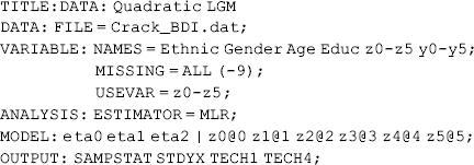
where the intercept (eta0), linear slope (eta1), and quadratic slope (eta2) growth factors are defined on the left-hand side of the ‘|’ symbol. The program automatically generates time scores of [0, 1, 4, 9, 16, 25] for the quadratic slope factor eta2.

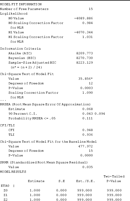
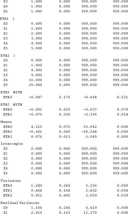
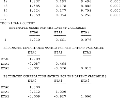
The mode results show a negative linear slope coefficient (Eta1 = −0.661, P < 0.001) and a positive quadratic slope coefficient (Eta2 = 0.076, P < 0.001), indicating that the growth curve of crack-cocaine use was nonlinear with a downward but concave up trend over time. Note that the correlation between the linear (eta1) and quadratic (eta2) latent slope growth factor is very high (r = −0.927) (see the TECHNICAL 4 OUTPUT section in Table 4.4). This is likely due to collinearity between the linear () and quadratic () polynomial time scores. We will deal with this problem in the next section.

Table 4.4 Selected Mplus output: quadratic linear LGM.

Centering time score at mean time: A common problem with polynomial measures of time is that its linear, quadratic and higher order terms are likely to be correlated. Hedeker and Gibbons (2006) illustrate that the linear time score (i.e., 0, 1, 2) and the quadratic time score (i.e., 0, 1, 4) in a quadratic trend model with three time points are nearly perfectly correlated. To deal with the collinearity, one can center the time variable or choose a midpoint of the observation period as the reference point for time. By centering time scores at mean time, the linear and quadratic time measures become (−1, 0, 1) and (1, 0, 1), respectively, and the correlation between the two time measures can be entirely removed.

Centering time score at the mean time is easy for an odd number of time points. For example, for a linear growth with five time points, by centering time scores at the mean time, we may code time scores like (−2, −1, 0, 1, 2). For an even number of time points that does not have an observed mid-time point, the following equation can be used for centering time score at the mean time:

(4.13)

where is the mean time of the observation time period. In our example, the original time scores were coded as (0, 1, 2, 3, 4, 5), and the mean time score is = (0 + 1 + 2 + 3 + 4 + 5)/6 = 2.5. Subtracting each time score by the mean time score, we have new time scores of (−2.5, −1.5, −0.5, 0.5, 1.5, 2.5); and the quadratic time scores can be readily calculated as (6.25, 2.25, 0.25, 0.25, 2.25, 6.25). The time scores will let the intercept growth factor represent the outcome measure at the mid-time point of the observation period (i.e., 15 months after baseline in our example). The corresponding Mplus program follows.

Mplus Program 4.5

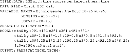
where the first BY statement in the MODEL command defines the intercept growth factor; the second and the third ‘BY’ statements define the linear and quadratic slope growth factors, respectively. The time scores for the quadratic slope factor are (6.25, 2.25, 0.25, 0.25, 2.25, 6.25), which are squared values of the linear time scores (−2.5, −1.5, −0.5, 0.5, 1.5, 2.5). Note that the [z0-z5@0 eta0 eta1 eta2] statement in the MODEL command sets the intercepts of the observed outcome variables to 0 and requests estimates of the latent growth factors.

The estimated mean of the intercept growth factor (eta0 = 3.030, P < 0.001) is the model estimated average frequency of crack-cocaine use when the time score equals 0. In other words, the mean frequency of crack-cocaine use at the middle point of the entire observation period was about 3.03. Using a centered time score, the correlation between the linear and quadratic latent slope growth factor was remarkably reduced from r = −0.927 to r = −0.305 (Tables 4.4 and 4.5).

Orthogonal polynomials: An alternative approach to deal with collinearity between polynomial time functions is to use orthogonal polynomials for time scores. Orthogonal polynomials are polynomials that are orthogonal to each other. For equal time intervals, the values of standard integer orthogonal polynomials can be found in statistics texts. In our example, for data with six time points (0, 1, 2, 3, 4, 5), the coefficients of integer orthogonal polynomials are given in Table 4.6, where iopt0, iopt1 and iopt2 are zero degree, first degree, and second degree integer orthogonal polynomial coefficients, respectively. Their corresponding regression coefficients would be the model intercept, linear slope, and quadratic slope of time. The corresponding Mplus program follows.

Table 4.5 Selected Mplus output: LGM with time scores centered at themidpoint of the observation period.

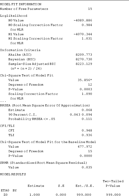
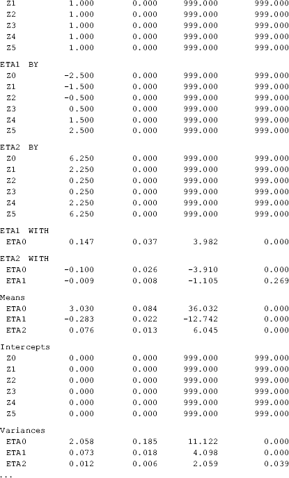
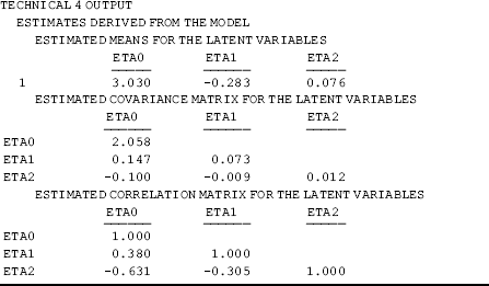
Table 4.6 Integer orthogonal second-order polynomials.

Mplus Program 4.6

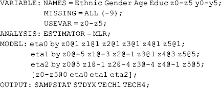
where the time scores for eta1 and eta2 are specified with the integer orthogonal polynomial coefficients. The selected model results are reported in Table 4.7.

Table 4.7 Selected Mplus output: quadratic linear LGM with integer orthogonal polynomials.

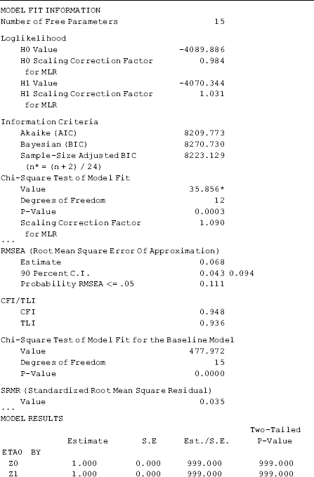
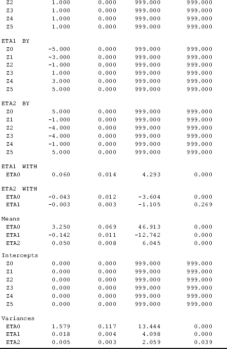
The intercept growth factor (ETA0 = 3.250, P < 0.001) of the integer orthogonal polynomial model represents the average outcome across time (Hedeker and Gibbons, 2006). In contrast, ETA0 = 3.030, P < 0.001 (Table 4.5) in the time-centered quadratic model is the average outcome at the midpoint of the observation period.

The integer orthogonal polynomial coefficients used in Mplus Program 4.6 are valid when time intervals are equal. A more general approach of calculating orthogonal polynomial coefficients, regardless of equal or unequal time intervals, is discussed and illustrated by Hedeker and Gibbons (2006). The ORPOL function in the SAS IML procedure can be used to compute these general orthogonal polynomial coefficients. For six time points as we have in our sample data, the following SAS program can be used to generate orthogonal second-order polynomials:

SAS Program 4.1

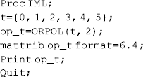
where a vector t, which contains the values of the original time score, was created first. Then the ORPOL function in the SAS IML procedure (i.e., interactive matrix language) is used to create general orthogonal polynomial coefficients. The option ‘2’ specified in the ORPOL function requests SAS to produce general orthogonal polynomial coefficients with the quadratic term as the highest order. The SAS output is shown in Table 4.8, where columns 1, 2 and 3 are the zero degree, first degree, and second degree general orthogonal polynomial coefficients, respectively. Their corresponding regression coefficients would be the intercept, linear slope, and quadratic slope growth factors. The corresponding Mplus program follows.

Table 4.8 SAS output for general orthogonal second-order polynomials.

Mplus Program 4.7

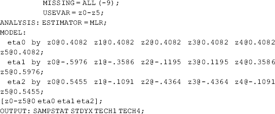
where the factor loadings for intercept factor (eta0), linear (eta1), and quadratic (eta2) slope factors are the general orthogonal polynomial coefficients estimated from SAS Program 4.1.

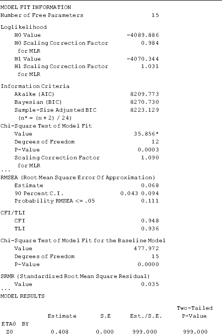
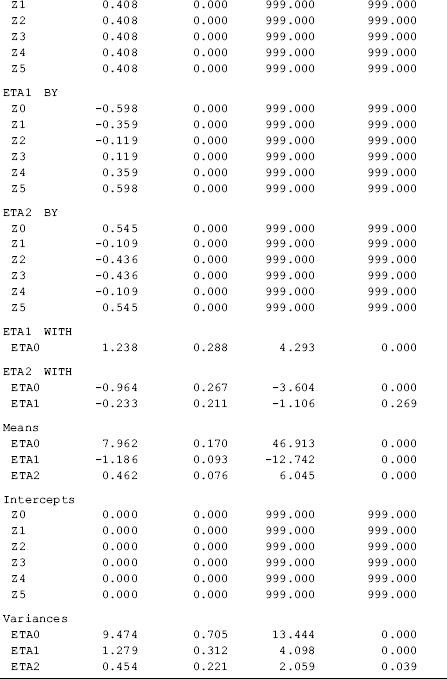
Note that the estimate of the intercept growth factor in this model, Eta0 = 7.962 (P < 0.001), is much larger than the previous estimate (e.g., Eta0 = 3.250) (Table 4.7). This is because the general orthogonal polynomial coefficients are rescaled measures of time scores. With six time points in this example, the zero-order polynomial coefficient 0.4082 is the square root of 1/6. The values in Column 1 in Table 4.8 are normalized, and their sum of squares equals 1.0 (Hedeker and Gibbons, 2006). Multiplying the intercept (i.e., Eta0 = 7.962) in Table 4.9 by 0.4082, we have Eta0 = 3.25, which is the same as the estimated mean value of Eta0 shown in Table 4.7. Similarly, the linear and quadratic growth factor means (Eta1 = −1.186 and Eta2 = 0.462) in Table 4.9 are different from those in the model with integer orthogonal polynomial coefficients (Eta1 = −0.142 and Eta2 = 0.050) in Table 4.7. We can multiply the coefficients by a constant, the ratio of the corresponding noninteger orthogonal polynomial coefficient to the integer orthogonal polynomial coefficient, to get the slope coefficient estimates [e.g., Eta1 = −1.186 * (−0.5976/−5) = −0.142, and Eta2 = 0.462 * (0.5455/5) = 0.050] that are the same as those shown in Table 4.7.

Table 4.9 Selected Mplus output: quadratic linear LGM with general orthogonal polynomials.

Piecewise linear LGM: Another method to deal with nonlinear growth trajectory is piecewise linear LGM. This approach breaks up the curvilinear growth into separate linear segments or pieces. Each segment has a separate slope, but is joined or tied to adjacent segments at fixed time points. The join points that mark one segment from the next are referred to as break points, interior knots, or knots. Knots give the curve freedom to bend and more closely follow the data. This approach is particularly appealing in the following situations: (1) when some nonlinear growth cannot be well approximated by polynomials of any order. For example, mean responses change (increase or decrease) rapidly in a time period and then slow down thereafter (or vice versa) (Fitzmaurice, Laird, and Ware, 2004); (2) when we are interested in comparing growth rates for two or more periods based on a substantial interest, such as growth rates before and after an intervention. A piecewise growth curve is sometimes referred to as a linear spline. There are many types of splines and estimation procedures. The analyses presented in this section focus on linear splines with predetermined knots (Greene, 1990; Wang et al., 1999).

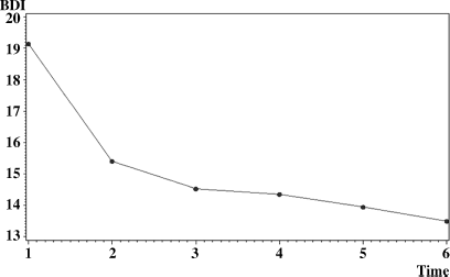
To fit a piecewise growth curve, it will be helpful to inspect the curvilinear growth pattern first to gain an idea of how many segments we should consider to model. Our data show there are two clear segments in a BDI score growth process (Figure 4.6): a sharp decline from the baseline to the first 6-month follow-up, and a steady slow decline thereafter. Thus, we would like to use BDI score (y₀ − y₅) as the outcome measures for demonstration of the piecewise LGM.

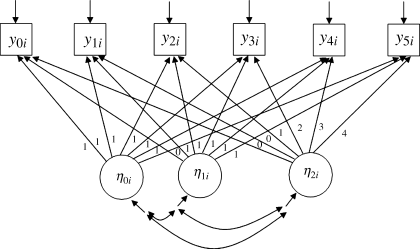
Once the number of segments is determined, we need to recode the time scores corresponding to the growth trajectories for each segment. Then two separate linear regressions are conducted simultaneously for each segment (e.g., baseline to 6-month follow-up, and from 6-month follow-up to 30-month follow-up). Therefore, one more latent slope growth factor, eta2, is added into the model to represent outcome change from t₁ (i.e., Month 6) to t₅ (i.e., Month 30) (Figure 4.7). The corresponding Mplus program follows.

Mplus Program 4.8

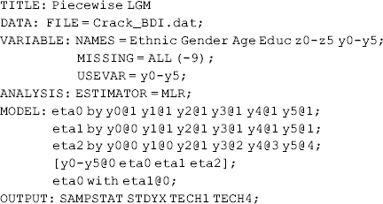
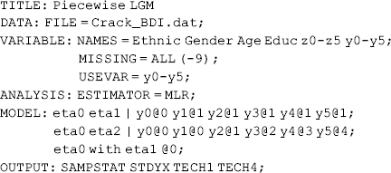
where the first BY statement in the MODEL command defines the intercept growth factor; the second BY statement defines the linear growth segment from t₀ to t₁; and the third BY statement defines the linear growth segment from t₁ to t₅. Since there are only two time points are involved in the first growth segment, the covariance between the intercept and the slope factor in the first growth segment was set to 0 (i.e., ‘eta0 with eta1@0;’) for the purpose of model identification.

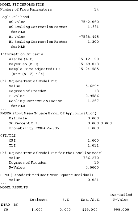
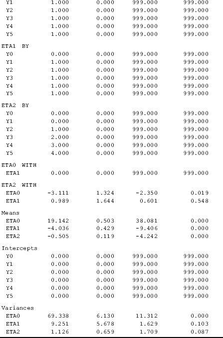
The average outcome measure (BDI score) at baseline was eta0 = 19.142; it declined by about 4 points (eta1 = −4.036, P < 0.001) in the first 6 months after baseline; after then the decline leveled off with a rate of change eta2 = −0.505 (P < 0.001) per 6-month period. As the outcome growth trajectory was specified to fit the observed growth pattern, the piecewise LGM fit data very well. In this example, it almost fits data perfectly: model = 5.629 (P = 0.9586), RMSEA = 0.000 (90% CI: 0.000, 0.000), P-value of the close test = 1.000, CTI = 1.000, TLI = 1.011, and SRMR = 0.021 (Table 4.10). If we add the PLOT command in the Mplus program, we will see the model estimated and observed growth curves would match almost perfectly.

Table 4.10 Selected Mplus output: piecewise LGM.

The following alternative Mplus program produces identical results for the above piecewise LGM.

Mplus Program 4.9

LGM with free time scores: Another approach allows for more flexible estimation of the trajectory of outcome growth over time by setting some of the factor loadings free. This kind of LGM is also called an ‘unspecified LGM.’ Freely estimating the time scores allows the shape of the growth trajectory to be determined by data, ending up with an empirically based nonlinear shape for outcome growth trajectory (McArdle and Anderson, 1990; Meredith and Tisak, 1990; Duncan and Duncan, 1994; Chou, Bentler, and Pentz, 1998; Wang 2004).

Figure 4.8 shows an unconditional two-factor LGM in which the time scores are model estimated. In such a model, at least two time scores must be fixed for the purpose of model identification. One time score must be fixed at zero to define the centering point. For example, by setting the time score at zero for t₀ (e.g., the time of baseline interview), t₀ would be referred to as the centering point, and the intercept growth factor would be, therefore, equal to y_0i. As aforementioned, different centering points can be chosen; that is, a time score can be set to zero at any time point, depending on how the centering point is interpreted.

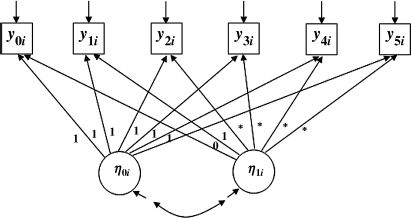
In addition, another time score in a two-factor unspecified LGM must be fixed at a nonzero value (usually 1.0) so that the measurement scale for the slope factor can be established. One unit on the scale of the time score is equivalent to the length of the observation time interval from time point t₀ to t₁. Thus, the estimated slope growth factor equals the amount of outcome change from time points t₀ to t₁. The time scores for time points t₂, t₃, t₄, and t₅ are set to be model estimated, and they are called free time scores. If a perfect linear trajectory is estimated, the estimated time scores for time points t₂, t₃, t₄, and t₅ should be 2, 3, 4, and 5, respectively. If the estimated value of the time score for t₂ was less than 2, it would indicate that the outcome change from observed time points t₁ to t₂ would be less than the expected linear change. On the contrary, if the estimated time score was greater than 2, it would indicate that the outcome change in this period would be larger than the expected linear change. The same principle applies to other sub-time periods (e.g., from t₂ → t₃, t₃ → t₄, and t₄ → t₅). As such, the model estimated time scores can be used as a tool for assessing literality of outcome growth trajectory (Wang, 2004, 2009). The following Mplus program is for the model specified in Figure 4.8.

Mplus Program 4.10

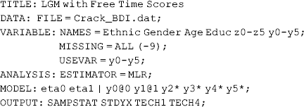
where y2^* y3^* y4^* y5^* (or simple y2 y3 y4 y5) in the MODEL command indicate that the time scores for t₂ − t₅ will be free parameters.

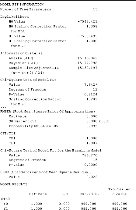
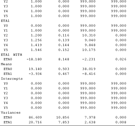
The model estimated time scores for time points t₂, t₃, t₄, and t₅ are 1.200, 1.256, 1.419, and 1.546, respectively, which are much less than the corresponding scores in a linear growth trajectory (i.e., 2, 3, 4, and 5). This indicates that the outcome measure (BDI score) had a nonlinear growth during the observation period: a rapid drop (eta1 = −3.934, P < 0.001) in the first 6-month observation period after the baseline interview; and then the decline leveled off for the rest of the observation period. From the model fit statistics and indices we can see that the model with free time scores fit data much better than predefined trajectory patterns, such as linear or quadratic growth.

Attention needs to be paid in interpreting outcome changes over time in the LGM model with free time scores. For example, in Table 4.11 the difference in time score between T₁ and T₂ is 1.2 − 1.0 = 0.2; as such the outcome change from T₁ to T₂ would be eta1^*0.20 = (−3.934)^*0.2 = 0.78.³

Table 4.11 Selected Mplus output: piecewise LGM with free time scores.

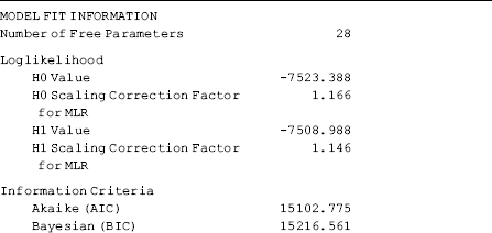
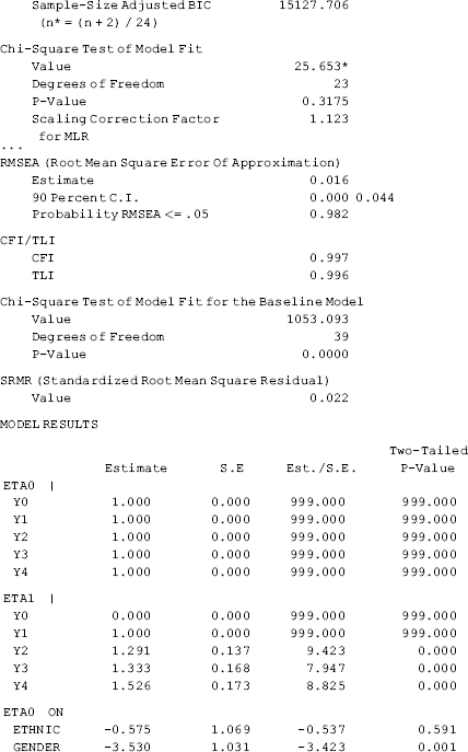
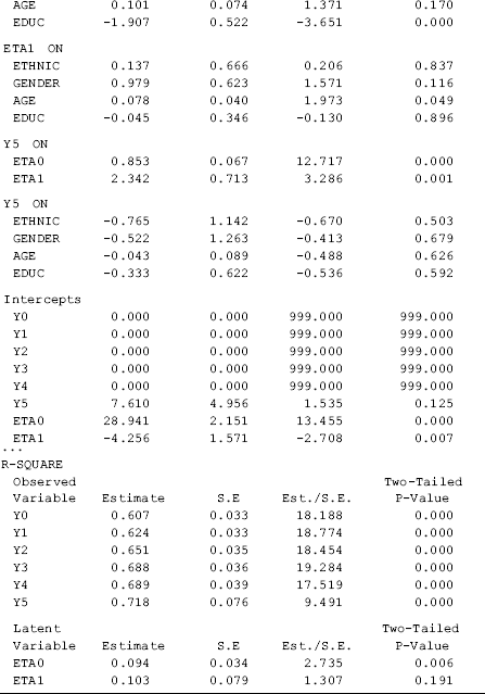
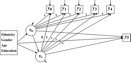
LGM with distal outcome: Very often thee is interest in how the growth trajectory of an outcome growth would affect a distal outcome measure at the end of the observation period. This can be readily implemented in a LGM. For example, in the model shown in Figure 4.9, we use the first five repeated outcome measures (i.e., y_0i − y_4i) to construct a LGM in the first 2-year period during the entire 30-month observation period, while treating the BDI score (i.e., y_5i) measured at the end of the observation period as a distal outcome. Certainly, a different distal outcome (e.g., a binary variable measuring severe depression) could be used in the model. The individual background characteristics and the latent growth factors are specified to predict the BDI defined depression at the end of the observation period. The following Mplus program is for the model specified in Figure 4.9.

Mplus Program 4.11

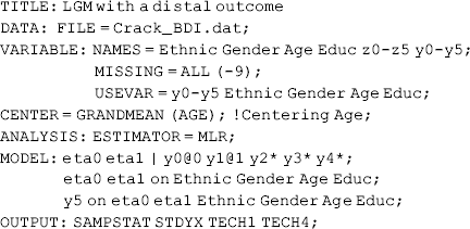
where the repeated outcome measures y₀ − y₄ are used to construct the growth trajectory of DBI score in the first 2 years (i.e., from baseline to the 24th follow-up interview); and then the latent growth factors are used to predict the distal outcome (y₅) at the end of the observation period (i.e., 30 months after the baseline in this study). The time-invariant covariates are used to predict both the growth factors and the distal outcome.

The interest of this model is to see how the BDI growth trajectory in the first 2-year observation period would affect the BDI defined depression at the end of the observation period. This is captured by regressing y₅ on eta0 and eta1, controlling for the socio-demographic covariates. The initial level of BDI score (i.e., eta0) and the rate of change in BDI score (i.e., eta1) in the first 2 years of the observation period had significant positive effects on y₅ (i.e., the BDI score at t₅) (0.853, P < 0.0001; 2.342, P = 0.001, respectively). Controlling for the growth factors, gender, ethnicity, age, and education have no significant effect on the distal outcome (Table 4.12).

Table 4.12 Selected Mplus output: LGM with distal outcome.