6.1 LCA Model

Traditionally, cluster analysis has been used to uncover homogeneous groups based on a set of observed variables. Different clustering methods can be used to identify relatively homogeneous groups of cases based on selected observed variables (Hartigan, 1975; Everitt, 1980; Aldenderfer and Blashfield, 1984). However, a major criticism of cluster analysis is that there are no statistical indices and tests, based upon which the number of clusters can be determined (Bergman and Magnusson, 1997; Steinley, 2003). As such, determination of the number of clusters is often done by examining tabular or graphical output, and researcher's subjectivity may bias the choice of a solution (Aldenderfer and Blashfield, 1984).

LCA is a model-based approach to cluster individuals/cases into distinctive groups (i.e., latent classes) based on their responses to a set of observed categorical variables (McCutcheon, 1987; Clogg, 1995; Muthén, 2001, 2002; Magidson and Vermunt, 2004; Collins and Lanza, 2010). LCA was initially introduced by Lazarsfeld (1950), and then further developed by Lazarsfeld and Henry (1968) and Goodman (1974). Due to the increasing availability of tremendous computing power and access to computer software for mixture models, LCA has been increasingly applied to various fields of social science studies.

Similar to the traditional cluster analysis techniques, the objective of LCA is to identify unobserved subgroups comprised of similar individuals. Unlike traditional cluster analysis, however, LCA is a model-based approach to clustering. It identifies subgroups based on posterior membership probabilities rather than somewhat ad hoc dissimilarity measures such as Euclidean distance. The general probability model underlying LCA allows for formal statistical procedures for determining the number of clusters, and more interpretable results stated in terms of probabilities. For details on the advantages of LCA over traditional cluster analysis, readers are referred to Magidson and Vermunt (2002).

As a form of latent structural modeling, LCA is somewhat similar to the CFA that we discussed in Chapter 2. Both LCA and CFA estimate latent variables from a set of observed indicator variables. However, the latent variables is continuous for CFA, but categorical (i.e., latent classes) for LCA. Continuous latent variables are usually referred to as factors, while categorical latent variables are referred to as latent class variables. Importantly, CFA focuses on grouping items, and thus is a variable-centered approach; in contrast, LCA focuses on grouping respondents or cases based on the patterns of item responses, and thus is a person-centered approach. The type of indicators/items used for CFA is very flexible; they could be continuous, binary, ordinal, nominal, count variables or any combination of these types of variables. Classical LCA models use categorical indicators/items; however, Mplus allows LCA to be conducted with categorical, continuous, and count indicator variables, as well as mixed combinations of these variables (Muthén and Muthén, 1998–2010). When continuous indicators/items are used for clustering, the model is usually called latent profile analysis (LPA) (Muthén and Muthén, 2000; Vermunt, 2004). In this section, we focus on LCA with categorical indicators/items.

Description of LCA model. Analogous to CFA, LCA uses underlying latent variables to describe the relationships among a set of observed indicators/items. In CFA, the observed indicators/items are assumed to be independent of each other once they are loaded up to their underlying factors. Similarly, the LCA also assumes such a local independence or conditional independence, that is, the observed categorical indicators/items are mutually independent once the categorical latent variable is conditioned out (McCutcheon, 1987; Clogg, 1995; Vermunt and Magidson, 2002).² Assuming the conditional independence, the joint probability of all observed indicator variables is described as:

(6.1)

From the above Bayes' formula, the posterior probabilities, which are analogous to factor scores in factor analysis, for each individual to be in different classes are estimated as (Muthén, 2001):

(6.2)

where two types of model parameters to be estimated in LCA modeling are shown: unconditional probabilities [, and is 1.0] and conditional probabilities [P(u_Q|C = k)]. As in factor analysis models, the model parameters of LCA are estimated adjusted for measurement errors. The unconditional probabilities are latent class probabilities, and the average of the probabilities can be interpreted as the prevalence of latent class (i.e., relative frequency of class membership) or the proportion of the population expected to belong to a latent class. The conditional probabilities are conditional item-response probabilities, representing the likelihood of endorsing specific categories/characteristics of the observed indicators/items, given a specific class membership. Like the factor loadings in factor analysis models, the conditional probabilities are measurement parameters in LCA. A conditional item-response probability equal or close to 1.0 indicates that members in the corresponding latent class endorse a category/characteristic of the item; on the contrary, a very small or zero conditional probability indicates that members in the latent class do not endorse the category/characteristic of the corresponding item. When a conditional item-response probability is close to value of 1/J, where J is the total number of categories in the item, the conditional probability is considered a random probability, thus the latent class membership is not predictive of the patterns of item responses. The conditional item-response probability is defined as:

(6.3)

where

(6.4)

which is the logit for u_qj given in latent class k. A logit L_jk = 0 indicates that the conditional item probability P_jk = 0.50; for an extreme value (e.g., L_jk = −15) the corresponding conditional item probability P_jk = 0.00; and for another extreme value (e.g., L_jk = 15), P_jk = 1.00. The conditional item-response probabilities provide information about how the latent classes differ from each other, and thus are used to define the estimated latent classes.

To estimate a LCA model, several steps are followed, including determining the optimal number of latent classes, examining the latent class classification, defining/labeling the latent classes, and predicting the latent class membership. In the following we briefly discuss the strategies of LCA modeling, and then use real data for model demonstration in the next section.

Determining the optimal number of latent classes in LCA. The number of latent classes in a LCA model is unobserved and cannot be estimated directly from a given data set. Determining the optimal number of latent classes is critical in LCA modeling. The familiar model fit statistics and indices, such as model χ², CFI, TLI, RMSEA, and SRMR are not available for assessing the goodness-of-fit of mixture models. To determine the optimal number of latent classes in a LCA model, usually a series of LCA models with increasing number of latent classes are fit and the optimal number of classes is determined by comparing k-class model with (k − 1)-class model iteratively. Note, to compare the LCA models with different number of latent classes, the LR test based on model χ² statistic is inappropriate. This is because the contingency table used for LCA with a set of observed categorical indicator variables usually has a large number of zero cells; as a result, the model χ² distribution is not well approximated. In addition, the (k − 1)-class model is a special case of the k-class model with one latent class probability being set to zero, that is, the value of one parameter being set on the border of the admissible parameter space, thus the difference of the log-likelihood between the two models doses not follow a χ² distribution (Muthén, 2004).

For model fit comparison or selection of the number of latent classes in mixture models, including LCA, several model fit indices and statistics are often used (Tofighi and Enders, 2008): (1) information criterion indices, such as AIC (Akaike, 1973, 1983), consistent AIC (CAIC; Bozdogan, 1987), sample-size adjusted CAIC (ACAIC), BIC (Schwarz, 1978), and ABIC (Sclove, 1987); (2) Lo–Mendell–Rubin likelihood ratio (LMR LR) test (Lo, Mendell, and Rubin, 2001), and adjusted LMR LR (ALMR LR) test; and (3) bootstrap likelihood ratio test (BLRT; McLachlan, 1987; McLachlan and Peel, 2000).

The information criterion indices that are based on the model log-likelihood and penalty terms related to model complexity and/or sample size are commonly used for comparing different LCA models. Mplus provides three types of information criterion indices: AIC, BIC and ABIC. Smaller values of information criterion indices indicate better model fit. A model with the lowest BIC and AIC is generally preferred. For complex models, one tends to favor AIC (Lin and Dayton, 1997).

On the basis of Vuong's (1989) study, Lo, Mendell, and Rubin (2001) have developed a LMR LR test, which is not based on χ² distribution, but a correctly derived distribution, to compare model fit improvement between models with k classes and (k − 1) classes. A significant P-value of the LMR LR test (e.g., P < 0.05) indicates a significant improvement in model fit in the k-class model compared with the (k − 1)-class model, thus rejecting the (k − 1)-class model in favor of a model with at least k classes. Then we need to further compare the (k + 1)-class model with the k-class model. If the LMR LR test is statistically insignificant (P ≥ 0.05), it indicates no more significant improvement in model fit by including an additional class into the model, and cannot reject the (k − 1)-class model; thus we may conclude that the optimal number of latent classes is (k − 1). The LMR LR test may inflate Type I error when sample size is small; as such, an ALMR LR test was proposed by adjusting model degrees of freedom and sample size (Lo, Mendell, and Rubin, 2001). However, a simulation study shows that the performance of the LMR LR and ALMR LR tests was virtually identical (Tofighi and Enders, 2008). Mplus provides both LMR LR and ALMR LR tests by using the TECH11 option in the OUTPUT command. Note that the LMR LR test has a normality assumption, and its performance needs more studies in the condition where the normality assumption is violated (Jeffries, 2003; Nylund, 2004).

An alternative LR test based on non-χ² distribution is the BLRT (McLachlan, 1987; McLachlan and Peel, 2000). Mplus provides such a test by using the TECH14 option. Parametric bootstrapping was used to generate a set of bootstrap samples using the parameter estimates from the (k − 1)-class model, and each of the bootstrap samples is analyzed for both k-class and (k − 1)-class models. Using all the bootstrap samples, a distribution of the log-likelihood differences between the k-class and (k − 1)-class models is constructed, and the BLRT is conducted based on this empirical distribution of the log-likelihood differences. The BLRT P-value is interpreted in the same way as that of the LMR LR test. Among all the approaches of determining the number of classes in a mixture model discussed above, simulation study shows that the BIC and BLRT perform the best (Nylund, 2004; Nylund, Asparouhov, and Muthén, 2007).

Examining the quality of latent class membership classification. Once the LCA model with the optimal number of latent classes is fit, individuals (cases or observations) are classified into the latent classes. The probability for an individual to be assigned to a specific latent class is measured by posterior class-membership probability given the individual's response pattern on the observed categorical indicators/items. The posterior class-membership probability in latent class k is defined in Equation (6.2), in which the probability that each individual belongs to each of the latent classes is estimated, and . The latent class memberships of individuals are not definitely determined, but based on their most likely latent classes on the basis of the estimated posterior probabilities; that is, they are classified into a latent class based on their highest posterior class-membership probabilities. If an individual's estimated largest posterior probability is close to 1.0, then the class misclassification or classification uncertainty is small for this individual. Suppose we have identified a 3-class LCA model, and the estimated posterior class-membership probabilities for an individual to be in Classes 1, 2 and 3 are 0.05, 0.06, and 0.89, respectively, then the individual is assigned to Class 3. For such a case, the probability of correct class-classification for this individual is about 0.89, and the probability of misclassification or classification uncertainty is about (0.05 + 0.06) = 0.11. If there were no misclassification for all individuals, the average posterior probability in a latent class would equal the population proportion of that latent class. In practice, however, misclassification is inevitable because the posterior probabilities are unlikely to be 1.0 for a specific class and zero for the rest of the classes. A rule of thumb for acceptable class classification is when the probability of correct class membership assignment is 0.70 or greater (Nagin, 2005).

Another criterion often used for assessing the quality of class membership classification is called entropy (Celeux and Soromenho, 1996), which is defined as,

(6.5)

where P_ik is the posterior probability for the ith individual to be in class k; EN(k) is a summary measure whose values ranges from 0 to 1 with smaller values indicating a better class classification or less classification uncertainty. Mplus does not provide such an entropy criterion, but a relative entropy criterion that is defined (Wedel and Kamakura, 2000; Dias and Vermunt, 2006) as:

(6.6)

where REN(k) is the relative entropy for a k-class LCA model with a sample size of N, which is a rescaled version of entropy. To be consistent with the Mplus User's Guide, we refer to REN(k) as the entropy in this book. The values of REN(k) range from 0.0 to 1.0, and a value closer to 1.0 indicates better classification. Though there is no clear cut-off point for the value of entropy to ensure a minimum level of good classification, Clark (2010) suggests a value of 0.80 is high, 0.60 is medium, and 0.40 is low entropy.

Once individuals are classified into latent classes, it is important to check the size of each class or the counts of individuals in each class. The relative class size or the percentage of individuals in each class represents the prevalence of the corresponding subpopulation in the target population. In order to have a meaningful class classification, the relative size of each latent class should not be too small. In addition, each of the latent classes must be theoretically meaningful and interpretable.

Defining latent classes. Just like the factor analysis model, the LCA model is also a measurement model. In exploratory factor analysis, once a set of latent variables/factors is extracted, the factors need to be meaningful and interpretable. Researchers need to define and name the factors based on how the observed indicators/items are loaded on factors. Similarly, once a set of latent classes is determined in a LCA model, each latent class must be meaningful and interpretable. The purpose of LCA is to use the estimated latent classes to describe the heterogeneity in the target population. The definition of a latent class is based on the patterns of item-response probabilities in that class. Thus, researcher should ensure that the model identified latent classes make substantive sense. If any latent class is not theoretically interpretable, the estimated model will not be useful regardless of model fit.

Predicting class membership. Covariates can be readily included in a LCA model to predict the latent class membership. Suppose we have P covariates (p = 1, 2,..., P), the relationships between the covariates and the latent class membership are modeled by a latent multinomial logit model as:

(6.7)

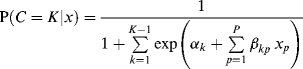
(6.8)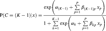

(6.9)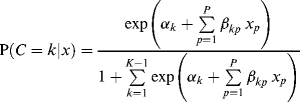

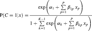
(6.10)

where there are (K − 1) logits, and the last class K is treated as the reference class with = 0 and = 0.

In traditional cluster analysis, clustering and estimation of the covariate effects on class membership cannot be conducted simultaneously. A common practice is to estimate the clusters first, and then merge the estimated class membership with the original data set to estimate the effects of covariates on the class membership. One of the advantages of LCA is that these two modeling processes can be conducted simultaneously. Excluding covariates from the LCA model is analogous to model misspecification in regression, and may result in distorted latent class membership estimation (Muthén, 2004). As such, in application of LCA one may start with testing the unconditional LCA model, and then include covariates into the model with ‘optimal’ number of classes. The latent class classification may not remain unchanged once covariates are included in the model. If this is the case, the model with covariates is preferred. However, a challenge arises if one wants to examine the relationship of latent class membership with a set of covariates and other outcome measures. We will demonstrate this further in the demonstration of our example LCA model.

Finally, it should be kept in mind that a well-known problem in LCA modeling, as well as in other mixture modeling, is that model estimation may not converge on the global maximum of the likelihood, but local maxima, thus providing incorrect parameter estimates (Goodman, 1974; Muthén and Shedden, 1999). As demonstrated in the next section, the solution is to estimate the model with different sets of random starting values to ensure the best likelihood (Muthén and Muthén, 1998–2010; McLachlan and Peel, 2000).

6.1.1 Example of LCA

The data used for demonstration of our LCA model were collected from a natural history study on rural drug use in Ohio (Falck et al., 2007). To be eligible for the study, participants had to meet the following criteria: (1) age 18 or older; (2) reside in one of the targeted counties; (3) not in drug abuse treatment or incarcerated; and (4) report the use of crack-cocaine, cocaine HCl, and/or methamphetamine, by any route of administration, at least once in the 30 days before the baseline interview. RDS was used for sample recruitment (Heckathorn, 1997, 2002; Wang et al., 2005, 2007). A total of 248 participants were recruited from three rural counties in Ohio.

It is well-known that drug users are likely to be involved in using a range of different drugs. LCA enables us to identify the typology of multi-drug use among the rural drug users. For the purpose of simplicity, we only use six binary measures of different drug uses in the past 6 months prior to the baseline interview: u1, marijuana; u2, methamphetamine; u3, crack-cocaine; u4, powdered cocaine; u5, opioids; and u6, hallucinogens. From Table 6.1 we can see that frequencies of drug use vary by drugs, but we do not know whether there exist heterogeneous subpopulations in the target population in regard to types of drug uses. Our interest is to identify distinctive typologies of drug uses among the drug users.

Table 6.1 Frequency of drug use.

Variable	N	%
u1 – Marijuana
No use	26	10.5
Use	222	89.5
u2 – Methamphetamine
No Use	151	60.9
Use	97	39.1
u3 – Crack-cocaine
No use	58	23.4
Use	190	76.6
u4 – Powdered cocaine
No use	48	19.4
Use	200	80.7
u5 – Opioids
No use	64	25.8
Use	184	74.2
u6 – Hallucinogen
No use	159	64.1
Use	89	35.9

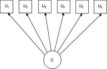
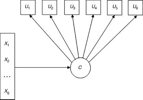
Figure 6.1 shows a diagram of an unconditional latent class model. Variables in boxes represent measured outcomes, u1–u6. The circled variable represents the unobserved latent class variable C. The local independence assumption for the LCA model implies that the correlations among the observed indicator variable u are fully explained by the latent class variable C, thus, no error covariances between the u variables are specified in the model. The model diagram depicted in Figure 6.1 looks like a CFA model, but the latent variable here is categorical, while it is continuous in a CFA model.

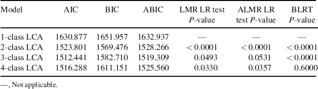
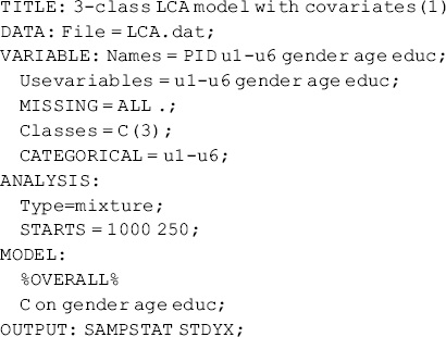
As the number of latent classes is unknown and cannot be directly estimated from a model, to identify the mode with optimal number of classes, various models with different number of latent classes need to be estimated and compared with each other. We start with a single class model, and then increase the number of classes by 1 each time. The model fit statistics/indices for the models with the number of latent classes ranging from 1 to 4 are reported in Table 6.2. The model with a single class has the largest AIC (1630.877), BIC (1651.957), and ABIC (1632.937) values, indicating this model fits data worse than all other models. In addition, the P-values of the LMR LR test, ALMR LR test, and BLRT in the 2-class model are all < 0.0001; this means that all the tests reject the single-class model in favor of a model with at least two latent classes. In other words, there exists heterogeneity in the target population in regard to drug use practices. In the 4-class model, the LMR LR and ALMR LR tests are statistically significant (P < 0.05), but the BLRT is not (P = 0.6000). That is, the first two tests are in favor of more than three classes, but the BLRT that is considered performing better than the LMR LR and ALMR LR tests (Nylund, Asparouhov, and Muthén, 2007) cannot reject the 3-class model. In addition, AIC, BIC, and ABIC are all smaller in the 3-class model than those in the 4-class model; thus we consider that the models with more than three classes are not preferred. Now, the preferred model must be either the 2-class or the 3-class model. On the one hand, the 2-class model has a smaller BIC (1569.476), but the 3-class model has smaller AIC (1512.441) and ABIC (1519.309); on the other hand, the ALMR LR test is in favor of the 2-class model (P = 0.0531), but the LMR LR test and BLRT (P = 0.0493 and P < 0.0001, respectively) reject the 2-class model. We tend to determine that the 3-class LCA model is the preferred model. We will show later that the classes identified by the 3-class model are very interpretable. The Mplus program for the 3-class LCA model follows.

Table 6.2 Comparison of different LCA models (N = 248).

Mplus Program 6.1

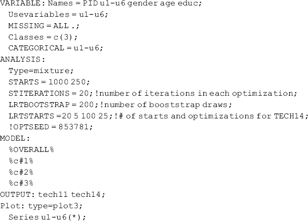
where the six binary indicator variables u1–u6 are specified in the CATEGORICAL statement of the VARIABLE command. The TYPE = MIXTURE statement is specified in the ANALYSIS command for mixture modeling. The default estimator is maximum likelihood with robust standard errors (MLR). In the MODEL command, the %OVERALL% statement specifies the overall model across all classes, while the statements %c#1%, %c#2% and %c#3% designate class-specific model specification. In our current example model, no model components were specifically specified for any particular class, thus the class specific statements %c#1%, %c#2% and %c#3% in the MODEL command are in fact not necessary in the above program.

As aforementioned, different sets of random starting values need to be used in mixture modeling to ensure model estimation converges on the global maximum of the likelihood, instead of local maxima. Once the TYPE = MIXTURE statement is specified in the ANALYSIS command, Mplus automatically generates 10 (by default) random sets of starting values in the initial stage optimizations for all model parameters except variances and covariances; and then maximum likelihood optimization is carried out for 10 (by default) iterations using each of the 10 random set starting values; and finally 2 (by default) starting values with the highest log-likelihoods in the optimization are used as the starting values for the final stage optimizations (Muthén and Muthén, 1998–2010). When more than two classes are specified in a LCA model (or other mixture models), it usually requests a larger number of random sets of starting values to avoid local maxima of the likelihood. The STARTS and STITERATIONS statements in the ANALYSIS command allow the user to specify selected numbers for the sets of starting values for the initial and final stages of optimizations, as well as for the number of iterations in each optimization. With the default settings of the starting values and iterations in our example, the Mplus output shows the following warning:

This suggests that model estimation does note converge on the global maximum of the likelihood and the number of starting values should be increased. Thus, in the above Mplus program we set STARTS = 1000 250 and ITERATIONS = 20; that is, we set:

• Number of random sets of starting values for initial stage optimizations = 1000.
• Number of random sets of starting values for final stage optimizations = 250 (about one-quarter of the number of initial starting values).
• Maximum number of iteration in optimization = 20.

The numbers we specified for the random starts in the STARTS and STITERATIONS statements here are arbitrary. In general the number of random starts should be large enough to ensure global maximum of model estimation; however, a large number of random starts will substantially increase the computation time.

After resetting the number of random starting values and iterations in the Mplus program, the warnings disappeared. However, this does not necessarily mean we have avoided local maxima. Usually, we need to check if the best log-likelihood value is replicated. In Mplus output, the final stage log-likelihood values are reported by initial stage start numbers and random seeds, ranked from the best log-likelihood values to the worst. Selected such values for our model are reported in the upper part of Table 6.3, where the first column is the final stage log-likelihood values, the last column is the random set number of initial starting values, and the middle column is the random seed that is a number used to initialize the random values.

Table 6.3 Selected Mplus output: unconditional 3-class LCA model.

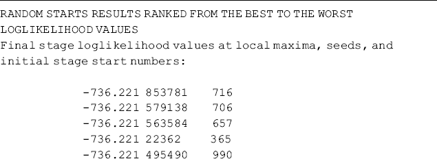
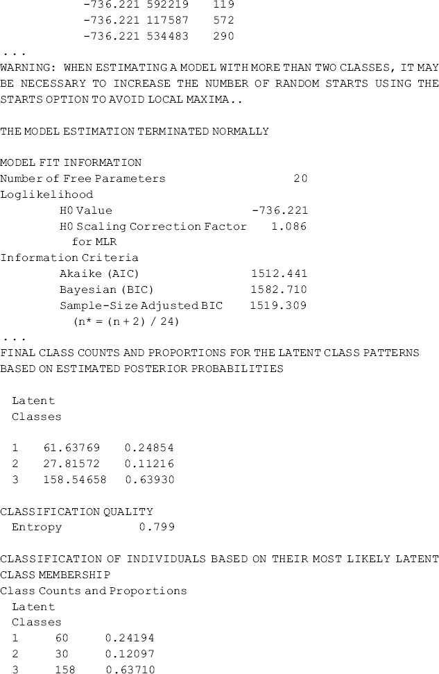
For the 250 sets of random starting values we specified for final stage optimizations, the best log-likelihood value of −736.221 was associated with the 716th set of initial random starting values, and the corresponding random seed is 853781. For a successful model convergence the best log-likelihood value should be replicated multiple times and is the most frequent solution. In our example, the best log-likelihood (i.e., − 736.221) was replicated 150 times, indicating a good model convergence. To make sure that model parameters were not estimated from local solutions, we can test the model by specifying different random seeds in the OPTSEED statement of the ANALYSIS command, and then check if the model parameter estimates are identical for different seeds. For example, we run our example model twice with different seeds: first, add statement OPTSEED = 853781, which is associated with the 716th set of random starts (see the upper part of Table 6.3), in the ANALYSIS command, and set STARTS = 0, then run the model. Do the same thing with another seed, for example, 579138, which is associated with the 706th set of random starts. The model parameters estimated using the two seeds are identical to those estimated from Mplus Program 6.1. This provides evidence that our model estimation has reached the global maximum of likelihood.

Now we turn to the TECH11 and TECH14 options in the OUTPUT command in Mplus Program 6.1. TECH11 requests the LMR LR test and the ALMR LR test, while TECH14 requests the BLRT. Attention needs to be paid to the results of TECH14. Very often, we see the following warning in the TECHNICAL 14 OUTPUT section of the Mplus output:

To ensure a trustworthy P-value for the BLRT, two options in the ANALYSIS command could be used in conjunction with the TECH14 option in the OUTPUT command: (1) Use the LRTBOOTSTRAP option (e.g., LRTBOOTSTRAP = 200 in our example) to increase the number of bootstrap draws.³ (2) Use the LRTSTARTS option to respecify the default numbers of the initial stage random starts and the final stage optimizations for the bootstrap generated data. The default numbers of the initial stage random starts and the final stage optimizations for the k-class model are 20 and 5, respectively. For the (k − 1)-class model, the default numbers are zeros for both the initial stage random starts and the final stage optimizations. We add LRTSTARTS = 20 5 100 25 statement in the ANALYSIS command to increase the default initial stage random starts and final stage optimizations to 20 and 5 for the (k − 1)-class model, and 100 and 25 for the k-class model, respectively.⁴

Note that the H0 Loglikelihood Value reported in TECH14 output is for the (k − 1)-class model. The value should be the same as the model H0 Loglikelihood Value estimated from the (k − 1)-class LCA model. For example, the TECH14 estimated H0 Loglikelihood Value shown at the bottom of Table 6.3 was −748.901, which is identical to the model H0 Loglikelihood Value estimated from our 2-class LCA model. If these two numbers are different, it indicates that we should increase the first two numbers specified in the LRTSTARTS option that are the number of random starts for TECH14 to estimate the (k − 1) model.

Once the number of latent classes is identified, we need to check and interpret the class classification. Two types of latent class counts and proportions are reported in the Mplus output: first, ‘FINAL CLASS COUNTS AND PROPORTIONS FOR THE LATENT CLASS PATTERNS BASED ON ESTIMATED POSTERIOR PROBABILITIES.’ These class counts are estimated based on the posterior class membership probabilities for each individual to be partially a member of all the classes, thus they are not integers. In out example, about 61.6 persons (24.9%) were assigned to Class 1; 27.8 persons (11.2%) to Class 2; and 158.5 persons (63.9%) to Class 3 (Table 6.3). Another type of latent class counts and proportions are estimated based on the most likely posterior class: ‘CLASSIFICATION OF INDIVIDUALS BASED ON THEIR MOST LIKELY LATENT CLASS MEMBERSHIP.’ That is, each individual is assigned to the most likely class (i.e., the class for which the individual has the largest posterior probability); thus the latent class counts are integers. If the two types of class counts substantially differ, it indicates that the class membership misclassification is large. With a perfect class membership classification (i.e., entropy = 1), the two types of latent class counts and proportions will be identical.

In out example, the class counts based on the most likely posterior class are 60 (24.2%), 30 (12.1), and 158 (63.7%) respectively, for the three classes (Table 6.3). The size and sample proportion of each class is not too small, and the correct class assignment probabilities are all above the cut-off point of 0.70 (Nagin, 2005): 0.91 for Class 1, 0.79 for Class 2, and 0.93 for Class 3. In addition, the entropy statistic, which is the summary information about the classification, has a value of about 0.80. We, therefore, conclude the latent class membership classification is adequate.

Some results in the Mplus output (e.g., the ‘Means’ by class in the Categorical Latent Variables section of Table 6.3) are not straightforward to understand. As a matter of fact, the ‘Means’ (e.g., C#1 -0.945; C#2 -1.740 in Table 6.3) are not the means of the latent classes, but the log odds of being in the kth class, compared with the reference class (the last class is treated as the reference class by default). In this unconditional LCA model, the log odds of being in the kth class is the intercept in Equations (6.7)–(6.10). The probabilities of being in latent Classes 1, 2, and 3 can be calculated as:

(6.11)

(6.12)

(6.13)

These figures match the proportions for the latent classes based on the estimated posterior probabilities (Table 6.3).

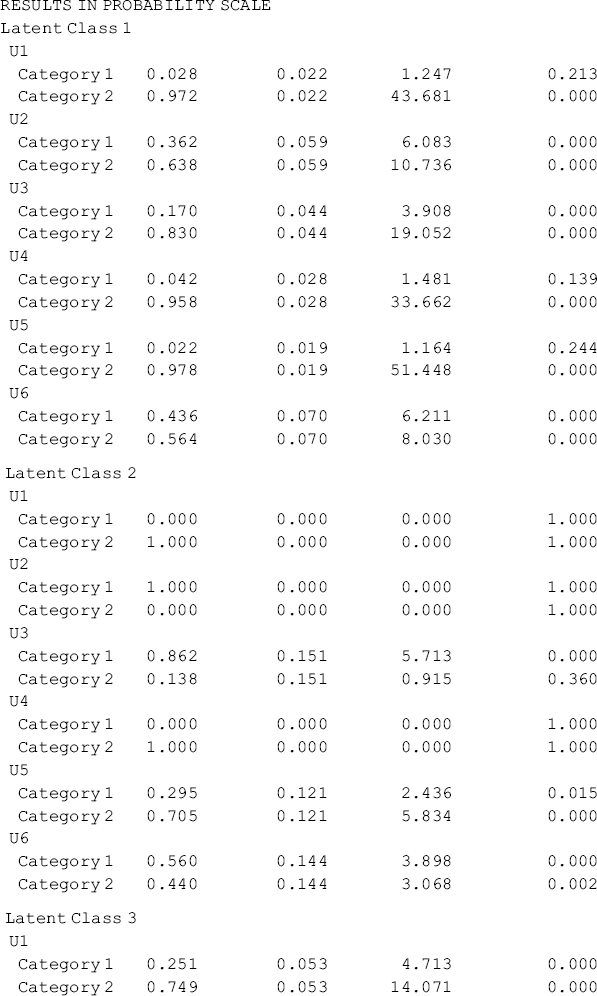
The Mplus output reported in the RESULTS IN PROBABILITY SCALE section in Table 6.3 are the estimated item response probability of endorsing each category of an indicator variable. The item response probability for the second category of each item (each item was coded in this example as: 0, no use; 1, use) is the conditional probability of using a specific drug, given in a specific class. The three classes are defined based on the pattern of item response probabilities. For example, for the 60 persons classified in Class 1, 100% of them used crack-cocaine (u3), and 72.7% of them used marijuana (u1) in the past 6 months prior to the baseline interview. In addition, about one-third of them used powdered cocaine (u4) and opioids (u5); but almost no one used methamphetamine (u2, 2.2%, P = 0.729) and hallucinogen (u6, 4.2%, P = 0.238). Therefore, we may define this class as crack-cocaine users. By the same token, we can define the second class as powdered-cocaine, and the third class as multi-drug users, while marijuana use was prevalent in each of the classes.

The unconditional and conditional probabilities shown in Table 6.3 are reorganized and reported in Table 6.4 by latent classes. The unconditional probabilities provide rich information about the patterns of drug use by latent classes. The majority (64%) of the rural drug users were multi-drug users (i.e., in Class 3). Over 90% of them used marijuana, powdered-cocaine, and opioids, 81% of them used crack-cocaine, and more than half of them used methamphetamine and hallucinogen. People in Classes 1 and 2 were crack-cocaine users and powdered-cocaine users, respectively. In addition, most of the people in all three classes were marijuana users. This detailed drug use information provides important implications for drug treatment/intervention for rural drug using populations.

Table 6.4 Unconditional and conditional probabilities: 3-class LCA model.

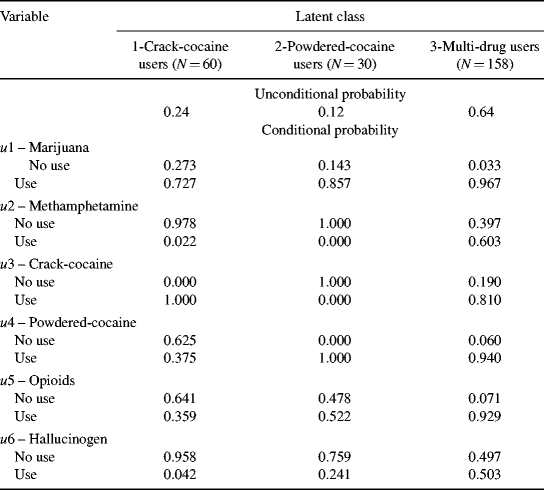
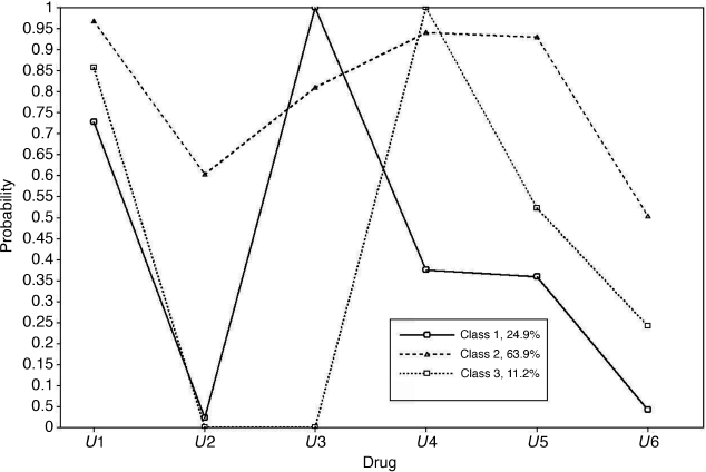
Figure 6.2, generated by using the PLOT command in Mplus Program 6.1, shows the profiles of drug use for 3-class LCA models. Mplus Graph allows users to edit the graphical displays of the plot, such as adding legend and x- and y-axis titles, editing axis labels, ranges, and line series, as well as to export the plot with different graphics file formats (e.g., JPG, EMF, and DIB). In Figure 6.2, the y-axis refers to the probability of using drug in the past six months prior to the baseline interview, while the x-axis lists indicator variables used for the LCA. The three lines represent the drug use patterns for the three latent classes. The average probability of using each specific drug shown in this figure match exactly the numbers reported in the FINAL CLASS COUNTS AND PROPORTIONS FOR THE LATENT CLASS PATTERNS BASED ON ESTIMATED POSTERIOR PROBABILITIES section in Table 6.4. Since the lines shown in Figure 6.2 cross each other, it indicates that the estimated latent classes differ in regard to type of drug use. If the lines were parallel to each other, it would indicate three classes with different degree (e.g., limited, moderate, and heavy drug use), rather than type, of drug use.

6.1.2 Example of LCA Model with Covariates

An extension of the LCA model is to include covariates (e.g., socio-demographic characteristics) to predict the latent class membership. The model is called the conditional LCA model (e.g., the model shown in Figure 6.3). The relationship between the latent class membership and the covariates are modeled by a latent multinomial logit model; and the classification and prediction of class membership are performed simultaneously. Theoretically speaking, covariates should be included in the LCA, otherwise, the model may be misspecified, leading to distorted parameter estimates (e.g., incorrect class membership probabilities) (Muthén, 2004). However, inclusion of covariates into a LCA often causes problems in model estimation. If some covariates do not have variation in any latent class, some regression coefficients in the multinomial logit mode will be undefined, ending up with some awkward estimates. In addition, some covariates that predict the latent class membership may also directly influence the observed outcomes (e.g., the u variables in our example). A significant direct effect of a covariate on a u variable indicates measurement noninvariant in the u variable with respect to the groups of people represented by the values of the covariates. This is similar to the differential item functioning (DIF) in the MIMIC model discussed in Chapter 3. Although measurement noninvariance in LCA can be handled (Asparouhov and Muthén, 2011), in applications of LCA it usually assumes measurement invariance and only covariates influence the latent class and indirectly influence the observed outcome variables via the latent class variable.

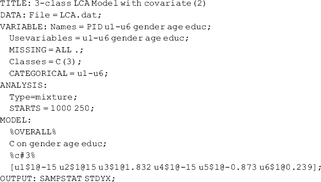
In the following, we demonstrate how to implement a conditional CLA model using the same data set LCA.dat. As aforementioned, inclusion of covariates in the model is likely to change class classification; therefore, LCA models with various numbers of latent classes were rerun and compared. Again, the 3-class model is the preferred model, and the corresponding Mplus program follows.

Mplus Program 6.2

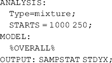
where three covariates (Gender, Age, and Educ) are included in the USEVARIABLES statement of the VARIABLE command. The ON statement in the MODEL command regresses the categorical latent variable C on the three covariates; as a result, a latent multinomial logit model is implemented to predict the class membership. Selected model results are shown in Table 6.5.

Table 6.5 Selected Mplus output: conditional 3-class LCA model.

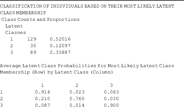
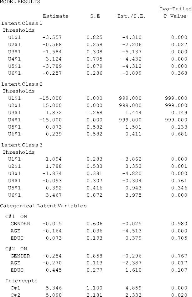
The class counts are: 129 (52.0%) for Class1, 30 (12.1%) for Class 2, and 89 (35.9%) for Class 3, respectively. Though the ordering of the latent classes changed and the class sizes are slightly different from those estimated from the unconditional LCA, the class definitions remain basically unchanged. In the conditional LCA, class classification and class membership prediction were implemented simultaneously. The results of the latent multinomial logit model are shown in the Categorical Latent Variables section of Table 6.5. Because the latent categorical variable has three categories (three classes), two logits were modeled, where Class 3 was treated as the reference group. Only Age has a significant negative effect in the multinomial model; that is, the younger drug users were more likely to be classified in Classes 1 and 2 rather than in Class 3. Mplus also provides alternative parameterizations for the multinomial model with different classes as the reference group (see the bottom of Table 6.5).

For the multinomial logit model in the conditional LCA, the last latent class (i.e., Class 3 in this example) with the 89 crack-cocaine users in the sample was treated as the reference group by default. If we want to use another class, for example, the latent class with the smallest class size (i.e., Class 2 in our example with 30 powdered-cocaine users) as the reference group in the model, we can reorder the latent classes in the following Mplus program.

Mplus Program 6.3

where the thresholds⁵ of the indicator variables estimated from Mplus Program 6.2 for the smallest class (N = 30) are specified in the last class instead of being freely estimated. It should be noted that once the class order has been changed, the results of the latent multinomial model should be interpreted differently. For example, the last class estimated from Mplus Program 6.3 will be the Powdered-cocaine users (N = 30), instead of Crack-cocaine users (N = 89); and this class will become the reference group in the multinomial model (model results are not reported here).

The results of Mplus Program 6.2 show that inclusion of covariates into a LCA model is likely to influence class classification. When a large number of covariates are included, it often causes model estimation difficulty for various reasons. For example, some covariates might not have much variation in some classes or might have direct effects on some observed outcome measures. Researchers often find that latent class formation keeps changing when different covariates are included and find it hard to identify the appropriate latent classes. As such, in real research, LCA is often based on unconditional LCA with no covariates; and then the estimated latent class membership is saved and merged with the original data set for further analysis using statistical packages, such as SAS, SPSS, or STATA. This practice is fine if the model estimated most likely class membership is adequate; that is, the entropy is high (0.80 or greater) (Clark, 2010).

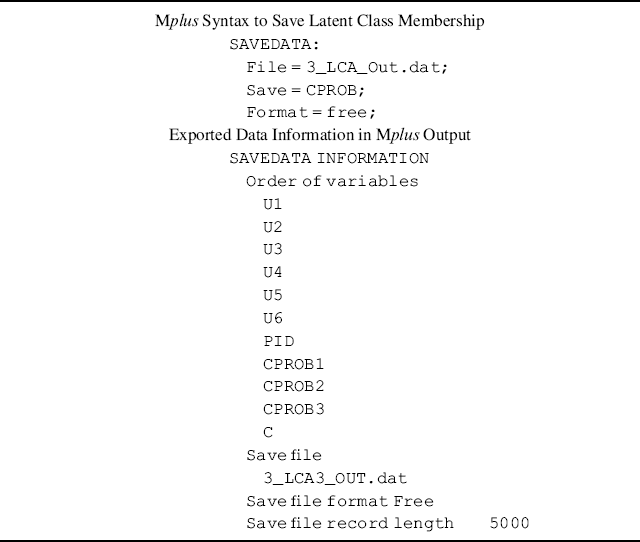
Mplus allows users to export a text data file which contains the original indicator variables, the estimated posterior probability of being in each specific latent class, and the class membership that an individual is assigned to. If we add the SAVEDATA command shown in the upper panel of Table 6.6 into the Mplus Program 6.1, the output information will be saved in a text data file named 3_LCA_OUT.dat. The data file will be saved in the folder where the Mplus program file is saved unless a particular folder is specified. It should be noted that in order to merge the exported data set with the original data, the personal ID or case ID variable (i.e., variable PID in this example) must be saved in the exported data set. This can be done by adding the IDVARIABLE = PID statement in the VARIABKE command. Data information for the exported data is provided at the bottom of the Mplus output (see the lower panel of Table 6.6).

Table 6.6 Saving Mplus output information for further analyses.

Alternatively, the posterior-probability estimated from an unconditional LCA can be used to examine the effects of covariates on the latent class membership without exporting estimated class membership. The AUXILIARY statement in Mplus allows variables to be specified that are not part of the LCA model to predict class membership based on pseudo-class draws from posterior probabilities. That is, the multinomial model is implemented after latent class classification, and inclusion of covariates will not affect latent class classification (Muthén and Muthén, 1998–2010). The following Mplus program demonstrates how this is done.

Mplus Program 6.4

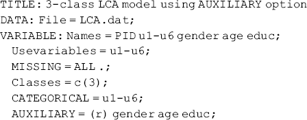
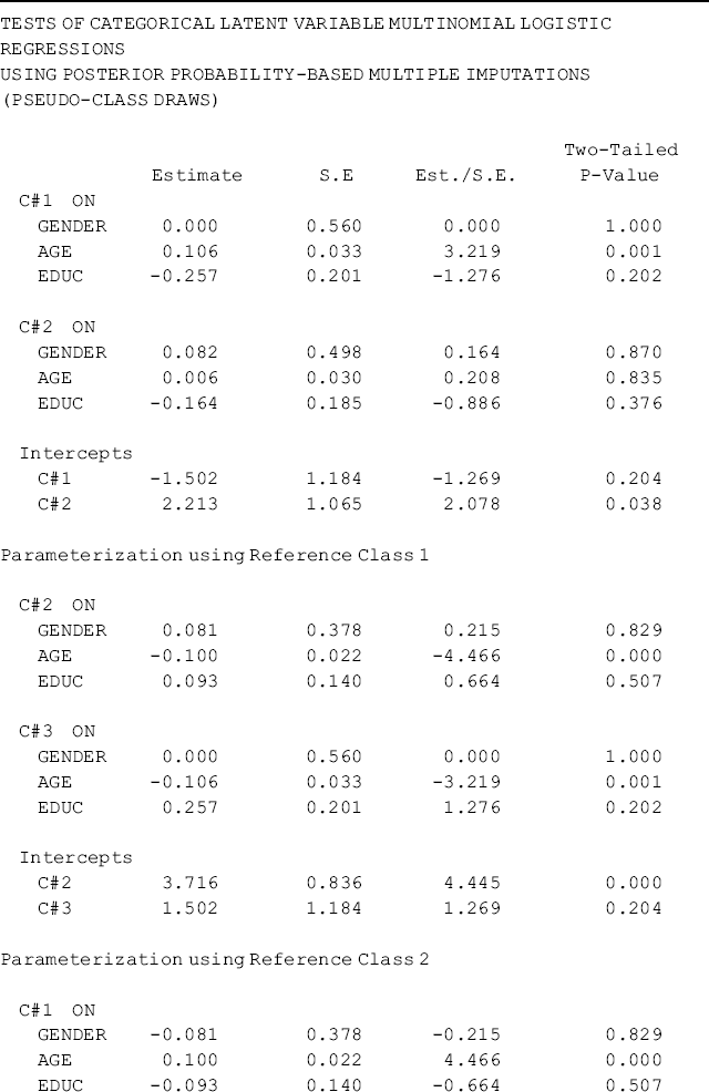
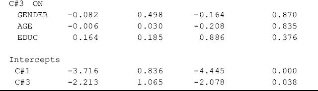
where covariates Gender, Age, and Educ are not included in the Usevariables statement, but in the AUXILIARY statement in the VARIABLE command. The letter r in parentheses is a specifier placed before all the variables that will be used as covariates in the multinomial logit model. Alternatively, the statement AUXILIARY = gender (r) age (r) educ (r), where the specifier is placed behind each variable, produces identical results. The results of the multinomial logit model are shown in Table 6.7 where different classes are treated as the reference group. The slope coefficients are interpreted in the same way as in the regular multinomial logit mode.

Table 6.7 Selected Mplus output: 3-class LCA model using AUXILIARY statement.

Different specifiers are available in the AUXILIARY statement for different purposes. For example, using specifier (e) in the AUXILIARY statement allows one to test the equalities of means of the covariates across latent classes⁶ (Muthén and Muthén, 1998–2010).

In this section we have discussed and demonstrated LCA models with categorical indicator variables. The same kind of model can be applied to continuous indicator variables, and the model is usually called latent profile analysis (LPA) model. Similar to LCA, the latent variables in the LPA model are also categorical and the model estimated unconditional probabilities are interpreted in the same way. Different from the LCA model, the latent classes in the LPA model are defined based on the mean values of item responses, instead of item response probabilities. For detailed comparisons between CFA, LCA and LPA, readers are referred to Gibson (1959), Lazarsfeld and Henry (1968), Bartholomew (1987), and Muthén (2002). In addition to continuous and ordinal measures, other types of indicator variables, such as nominal, censored, and count variables, as well as a combination of different variable types can also be used for mixture modeling (Muthén and Muthén, 1998–2010).