6.3 Growth Mixture Model

In Chapter 4 we discussed LGM in which outcome growth trajectory over time is captured by continuous latent variables (i.e., latent intercept and slope growth factors). LGM assumes that all individuals in the sample are from a single homogeneous population, and individual growth trajectories vary randomly around the overall mean growth trajectory. Very often, the assumption of homogeneity in outcome growth trajectory is unrealistic. Ignoring possible growth heterogeneity and focusing on the overall mean growth trajectory can lead to misunderstanding and wrong conclusions about outcome growth. In this chapter we extend LGM to the GMM to assess whether the population under study is comprised of a mixture of identifiable subpopulations/groups based on their growth trajectories (Verbeke and Lesaffre, 1996; Muthén and Shedden, 1999; Muthén and Muthén, 2000; Muthén, 2001, 2002, 2004>, >, >). The GMM model has increasingly gained in popularity in longitudinal studies in different fields of social sciences and public health studies because of its capability of enabling the examination of possible heterogeneity of outcome growth trajectories; classifying individuals into distinctive growth trajectory groups; and relating the heterogeneous growth trajectories to distal outcomes.

Figure 6.5 is helpful to compare growth trajectories modeled in the LGM and the GMM. Figure 6.5a illustrates hypothetical growth trajectories in which each line represents an individual's growth trajectory, and different individuals have different intercepts and slopes. The bold line represents the overall average growth trajectory. This kind of outcome growth trajectory is modeled in the LGM discussed in Chapter 4. In the LGM outcome growth trajectories vary around the overall average growth trajectory, assuming that all individuals in the sample come from a single population. Individual variations around the overall mean growth trajectory (the bold line in Figure 6.5a) are captured by the random intercept and slope coefficients.

Figure 6.5 Outcome growth trajectories in LGM and GMM.

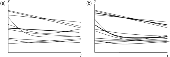
The LGM can be generalized to a GMM that accommodates population heterogeneity in the outcome growth by classifying individuals into different trajectory groups/classes. The LGM uses continuous latent variables (i.e., latent growth factors) to summarize outcome growth trajectories over time. The GMM further identifies the patterns of outcome growth trajectories by employing a categorical latent (i.e., latent class) variable; that is, the GMM uses both continuous and categorical latent variables to represent outcome growth. For example, Figure 6.5b illustrates three trajectory groups:

• Group 1: low initial level of outcome and no significant change in the outcome over time;
• Group 2: moderately high initial level of outcome and significant nonlinear change in the outcome;
• Group 3: high initial level of outcome and rapid linear change in the outcome.

Clearly, the overall average growth trajectory (the bold line in Figure 6.5a) ignores the growth heterogeneity and provides misleading information about outcome change over time.

From an intuitive perspective, we may consider that the GMM is implemented in two steps though the two steps are in fact conducted simultaneously in model estimation: first, individual growth trajectories are estimated from the LGM, and then individuals are clustered, based on the estimated continuous latent intercept and slope growth factors, into a finite number of groups/classes in a categorical latent variable. Growth trajectories are similar within the group/class, but different across groups/classes. Using a combination of continuous and categorical latent variables, the GMM has clear advantages over the LGM. GMM not only models intra-individual growth trajectories and inter-individual variations in the trajectories, but also accommodates population heterogeneity in outcome growth trajectory by identifying distinct groups within which individuals share similar growth trajectories.

Like the LGM model, the GMM can be described similarly in multilevel model notation. The following model can be specified for each of the K latent classes in a GMM model:

(6.34)

where in the level 1 model represents the observed outcome variables for case i at time t for latent class k. The parameters in both level 1 and level 2 equations are all class-specific. The two latent growth factors and are two continuous latent variables; represents time scores, which can be specified as linear, nonlinear polynomial functions of time, or free time scores. The residual term is a composite error term at time t, representing both random measurement error and time specific influence of the ith individual; intercept coefficients at level 2 model and represents the model estimated overall mean levels of the initial outcome and the average rate of outcome change over time; the slope coefficients and are the fixed effects of covariates on the latent intercept and slope growth factors; and and are error terms representing between-subject variations in the latent growth factors. Growth trajectory in each growth trajectory class could be either linear or nonlinear, and the trajectories could be noninvariant or invariant across classes, depending on the nature of the population under study. The following sections demonstrate applications of GMM using real research data.

6.3.1 Example of GMM

The data used for demonstration of LGM models in Chapter 4 is used again for demonstration of GMM models in this section, studying (1) whether there are different patterns of crack-cocaine use in a 30-month observation period; (2) what individual characteristic would affect the outcome growth and the pattern of the growth trajectories; and (3) whether the different patterns of growth trajectories of crack-cocaine use would be related to the depression status at the end of the observation period. The outcome variables involved in the modeling are crack-cocaine use frequency measured at six time points t₀ − t₅; covariates are Gender, Ethnic, Age, and Educ; and distal outcome – BDI defined depression status.⁹

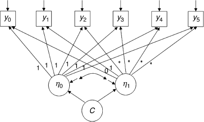
We start with the unconditional GMM model shown in Figure 6.6, in which six repeated measures (y₀ − y₅) of crack-cocaine use frequency are used as the indicator variables of the latent growth factors and . In the model, outcome growth function (linear or nonlinear) will be determined by data since the time scores are set as free parameters (see Section 4.2), and the continuous latent growth factors and are treated as the indicators of the latent categorical variable – latent class variable C, in which latent growth trajectories vary between classes, as well as within classes.

Figure 6.6 Unconditional GMM.

To implement the GMM, we need to go through the same process as implementing the LCA. Namely, we need to determine the optimal number of latent trajectory classes, examine the quality of latent class membership classification, define the latent trajectory classes, and predict latent class membership, and so on. The following GMMs with progressively larger number of latent trajectory classes were estimated and compared.

The model fit statistics/indices of the models under comparison are shown in Table 6.17. The model with a single class has the largest AIC (8205.052), BIC (8266.009), and ABIC (8218.408) values, indicating its fit is the worst. In addition, the LMR LR test, ALMR LR test, and BLRT in the 2-class all have a P-value < 0.05, suggesting to reject the single-class model in favor of at least two classes. The results provide evidence that the growth trajectory of crack-cocaine use among the drug users was not homogeneous, but heterogeneous. The next step of our modeling is to determine the optimal number of the latent trajectory classes. By comparing the GMMs with Classes 2, 3, 4, and 5, the 4-class GMM has the lowest BIC (8102.923), and the BLRT of the 5-class GMM cannot reject the 4-class model (P = 0.0946). Since BIC and BLRT are considered performing the best among the approaches of determining the number of classes in mixture modeling (Nylund, Asparouhov and Muthén, 2007), the 4-class GMM is favored.

Table 6.17 Comparison of different GMMs (N = 430).

The Mplus program for the 4-class GMM follows:

Mplus Program 6.8¹⁰

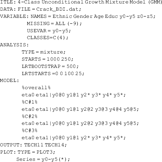
where the data set named Crack_BDI.dat that was used for model demonstration in Chapter 4 is retrieved from the folder where the Mplus Program 6.8 is saved. The repeated measures of crack-cocaine use frequency named as y₀ − y₅ are used for the unconditional GMM. Free time scores are specified in the %OVERALL% MODEL command to allow the outcome growth trajectory to be determined by data. Note that the growth trajectory specified in the %OVERALL% model statement is a default specification. If no further growth trajectory specification is given in the class-specific MODEL commands, then Mplus would produce the same growth trajectory for all the classes. In the Mplus Program 6.8, we specified linear growth in the %C#1% and %C#2% class-specific MODEL commands for Classes 1 and 2, and free time scores for Class 3. As no time scores were specified for Class 4, its growth trajectory will be defined by the %OVERALL% MODEL command by default.

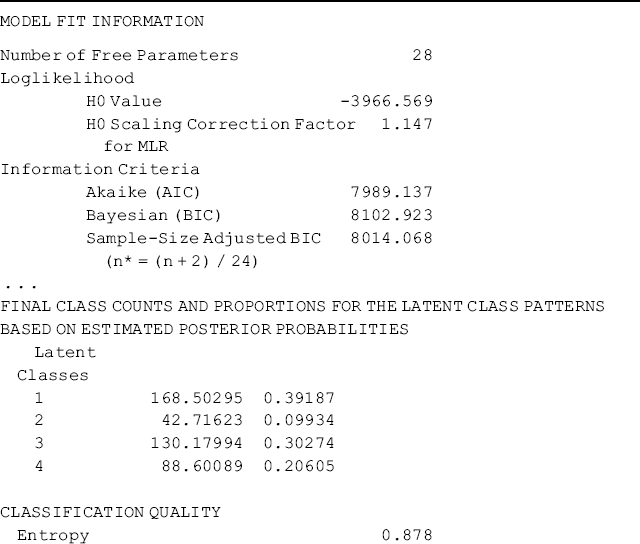
Selected model results are shown Table 6.18. Individuals in the sample were classified into four classes, each of which has different growth trajectory, in regard to crack-cocaine use frequency over time. Of the total 430 cases, 38.1% (N = 164) were classified¹¹ in Class 1, 11.2% (N = 48) in Class 2, 32.3% (N = 139) in Class 3, and 18.4% (N = 79) in Class 4, respectively. The quality of latent class membership classification is good: first, the entropy statistic is high (0.878); and secondly, the diagonal figures in the matrix of the Average Latent Class Probabilities for Most Likely Latent Class Membership in Table 6.18 are all much higher than 0.70, the rule of thumb for acceptable class classification (Nagin, 2005).

Table 6.18 Selected Mplus output: 4-class unconditional GMM.

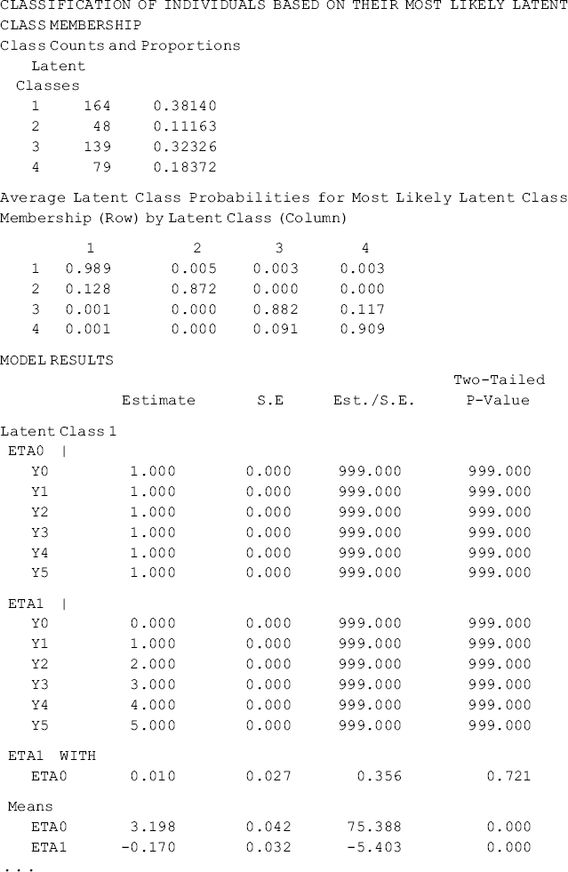
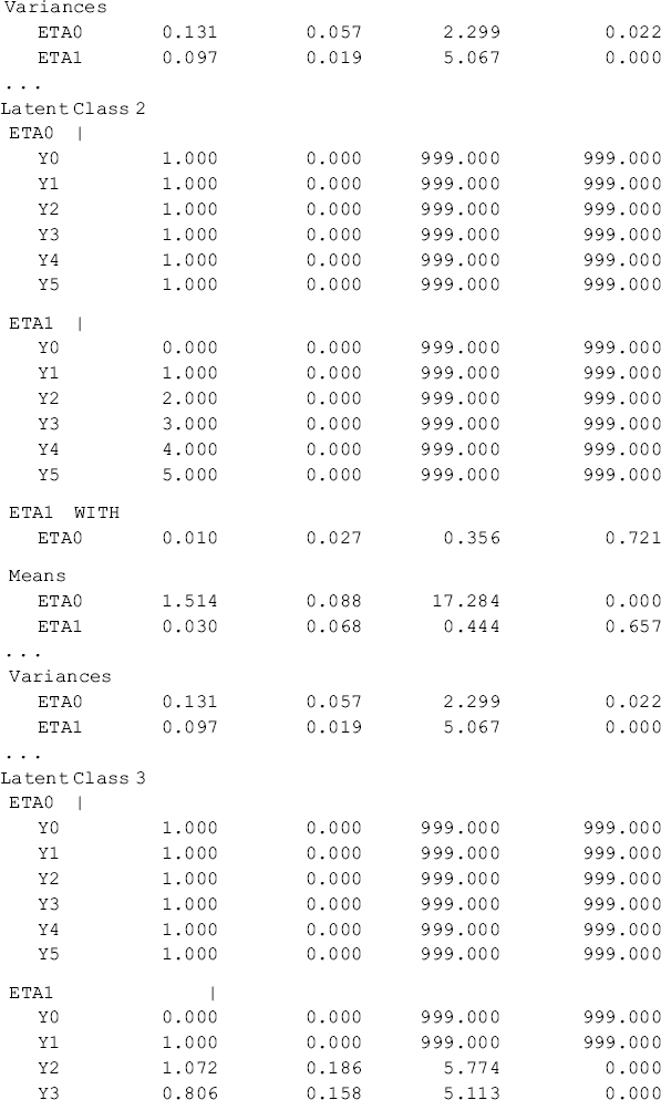
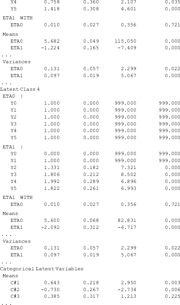
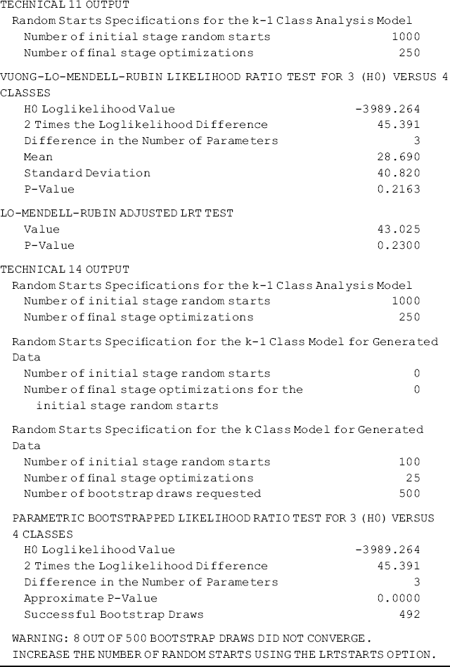
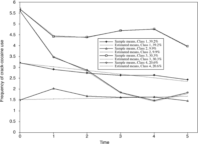
The observed and model estimated growth trajectories of crack-cocaine use frequency are shown by class in Figure 6.7. The solid lines represent observed growth trajectories, and the dashed lines represent the model predicted trajectories. From the growth trajectories depicted in Figure 6.7, we can define Class 2 as lighter crack users who reported using crack no more than once a week¹² and kept the same practice over time without significant change. The corresponding latent growth factors are: eta0 = 1.514 (P < 0.0001) and eta1 = 0.030 (P = 0.657) (see the panel of Latent Class 2 in the MODEL RESULTS section of Table 6.18). Class 1 can be defined as moderate crack users among whom the average initial level of crack-cocaine use was eta0 = 3.198 (P < 0.0001) and their crack use frequency declined over time at a rate of eta1 = −0.17 (P < 0.0001). Individuals in Classes 3 and 4 were all heavy crack users at baseline [the estimated latent intercept growth factor eta0 = 5.60 (P < 0.0001) and eta0 = 5.68 (P < 0.0001), respectively]. Among people in Class 4, crack-cocaine use frequency declined rapidly over time (the latent slope growth factor eta1 = − 2.092, P < 0.0001) and reached a very low level at the end of the observation period (Figure 6.7). Individuals in latent Class 3 are most problematic. Although their drug use frequency reduced significantly (eta1 = − 1.224, P < 0.0001), on average individuals in this class still used crack-cocaine on a daily basis (the measure of crack use frequency was still greater than 4 at the end of the observation period; Figure 6.7). The interpretation of the estimates of the latent growth factors is straightforward for the two linear trajectories in Classes 1 and 2. The growth trajectory functions in Classes 3 and 4 were data determined by specifying free time scores in the growth model in each of the classes. Details of interpretation of such parameter estimates were discussed in Chapter 4.

Figure 6.7 Latent growth trajectories by class: 4-class unconditional GMM.

At the end of the MODEL RESULT section in the Mplus output shown in Table 6.18, we see a panel of Categorical Latent Variables where Means are reported for specific classes. This output often puzzles new users of Mplus. In our unconditional GMM, the Means reported for latent Classes 1, 2, and 3 are in fact the estimated logits of the latent class multinomial model; that is, the estimated log odds of being in Classes 1, 2, and 3, compared with the reference class (the last class, i.e., Class 4 in this example, is treated as the reference class by default). The probabilities of being in Classes 1, 2, 3 and 4 can be calculated as:

(6.35)

(6.36)

(6.37)

(6.38)

The calculated class probabilities are in fact the estimated proportions of the latent class patterns based on estimated posterior probabilities, instead of the most likely latent class membership (see the corresponding figures in the FINAL CLASS COUNTS AND PROPORTIONS FOR THE LATENT CLASSES BASED ON THE ESTIMATED MODEL section in Table 6.18).

In this section we have demonstrated an unconditional GMM with different growth trajectories in latent growth classes. As the class membership classification is adequate (entropy > 0.80) (Clark, 2010), we may use Mplus's SAVEDATA command (Table 6.6 or Table 6.16) to export and merge the estimated class membership with the original data set; as such, the relationships between the class membership and covariates, as well as other outcome measures, can be easily analyzed using standard statistical packages, such as SAS, SPSS, STATA, and so on. However, it is recommended to conduct latent class estimation and class membership prediction simultaneously since excluding covariates from a GMM may lead to model misspecification, thus leading to distorted model results (Muthén, 2004). In addition, the SAVEDATA command does not export the latent growth factor estimates. Researchers would very often like to include covariates into a model to predict latent class membership, as well as to predict the within-class variation of the growth trajectories. Finally, it is also interesting to examine whether and how the estimated outcome growth trajectory patterns would predict distal outcomes. In the following section, we include some time-invariant covariates and a distal outcome into the GMM.

GMM model with covariates and distal outcome. In this section, our conditional GMM will provide information to answer the following research questions: how individual social-demographic characteristics influence the patterns (latent classes membership) of the growth trajectories of crack-cocaine use over time; how the covariates influence the growth trajectory within each latent growth class; and whether the patterns of the growth trajectories (latent class membership) influence depression status at the end of the observation period – a distal outcome.

The GMM with covariates and a distal outcome is depicted in Figure 6.8 Four social-demographic variables Ethnicity, Gender, Age, and Education (the definitions of the variables are given in Section 4.1) are included to predict the latent class membership, as well as the latent growth factors (i.e., the latent intercept growth factor eta0 and the latent slope growth factor eta1) within each class. In Figure 6.8 there are two dotted lines from the latent class variable C ending on the lines that go from covariates to the two continuous latent variables eta0 and eta1. These dotted lines indicate that the effects of the covariates on eta0 and eta1 vary across latent classes or the interactions between the covariates and the latent class variable. Recall from Chapter 5 that interactions between covariates and the observed group membership mean that the effects of covariates on outcome measures vary across the observed groups. Here we are talking about interactions between covariates and latent class variable C.

Figure 6.8 GMM with covariates and distal outcome.

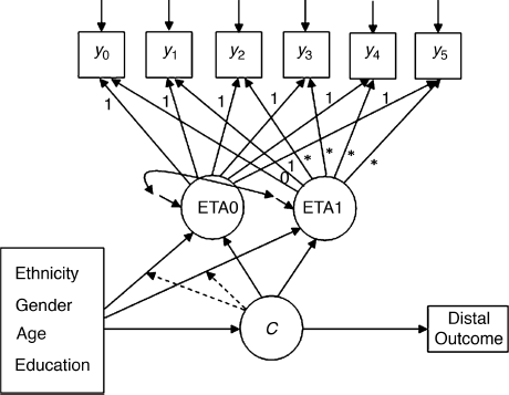
A distal outcome variable, Depression, is also included in the model that is the depression status measured at the end of the observation period (i.e., t₅, the 30-month follow-up). The influence of growth patterns of crack-cocaine use over time on the distal outcome will be examined by regressing Depression on the latent class variable C in the model.

The Mplus program for the GMM with covariates and distal outcome follows:

Mplus Program 6.9

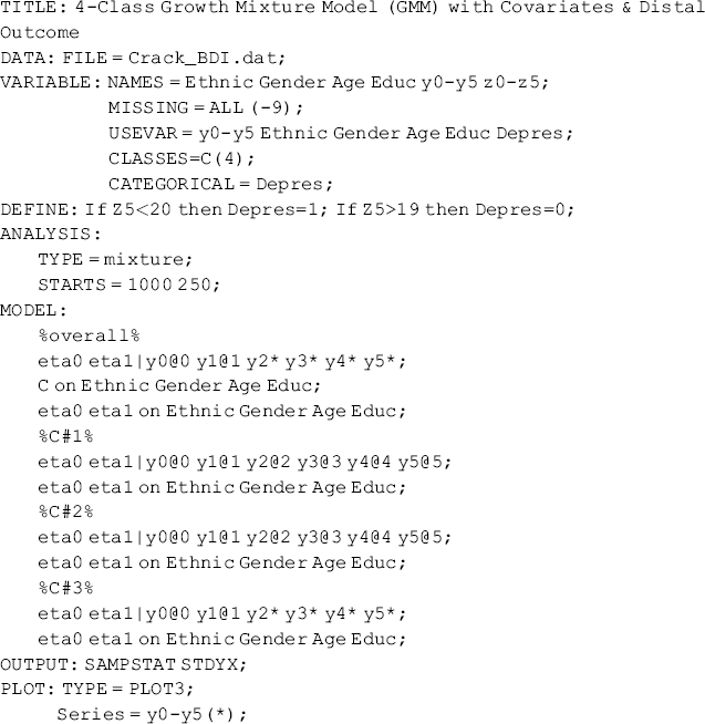
where the DEFINE command is used to create a binary variable Depres based on variable z5, which is the BDI score (see Chapter 4 for a description of BDI) measured at the end of the 30-month observation period. To model probability of having no depression at time t₅, the binary distal outcome variable was coded as 1 for no depression, and 0 otherwise. The first ON statement in the overall MODEL command specifies a multinomial logit mode regressing the latent class variable C on the covariates Ethnic, Gender, Age and Educ. Since the latent class variable has four categories, three logits will be modeled with the last category (i.e., Class 4) as the reference group by default. The second ON statement in the overall MODEL command regresses the continuous latent variables eta0 (i.e., the intercept growth factor) and eta1 (i.e., the slope growth factor) on the covariates. This linear regression statement is repeatedly specified in each of the class-specific MODEL commands to release the default equality restrictions on the regression coefficients. As no class-specific command is specified for Class 4 in the Mplus program, model specification for Class 4 is done by the overall MODEL command by default.

Note that the binary distal outcome Depres is listed in the used variables in the USEVAR statement of the VARIABLE command, but not specified in the MODEL command. Mplus will automatically estimate the proportion of each category of the binary variable Depres by class. If the distal outcome is a continuous variable, then its mean value will be estimated for each class. The effects of the covariates on the distal outcome can also be readily tested by using the ON statement in the MODEL command, specifying a regression of the distal outcome on the covariates. If we specify regression of Depres on Ethnic, Gender, Age, and Educ in the overall MODEL command, Mplus will produce the same set of regression coefficients for each class; if regressions are specified in class-specific MODEL commands, different sets of regression coefficients will be produced. In the current example model, we are only interested in the relationship between the latent class membership and the distal outcome; the effects of covariates on the distal outcome were not tested.

Selected model results are shown in Table 6.19. It is noticeable that once the model specification is modified (e.g., covariates and/or distal outcome are included in the model), the class membership classification is likely to change to some extent. In our example, the estimated outcome growth trajectories of the conditional GMM are depicted by class in Figure 6.9.¹³ The patterns of the outcome growth trajectories estimated from the GMM with covariates and distal outcome were similar to those in the unconditional GMM. Thus, the definitions of the latent classes basically remain unchanged. However, the estimated latent class counts and proportions are somewhat different between the conditional and unconditional GMMs (Tables 6.18 and 6.19). According to Muthén (2004), exclusion of covariates and distal outcome from GMM may lead to model misspecification, resulting in distorted model results. As such, the class membership classification shown in Figure 6.9 and Table 6.19 are preferable.

Figure 6.9 Latent growth trajectories by class: 4-class GMM with covariates and distal outcome.

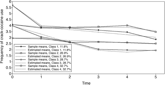
Table 6.19 Selected Mplus output: GMM with covariates and distal outcome.

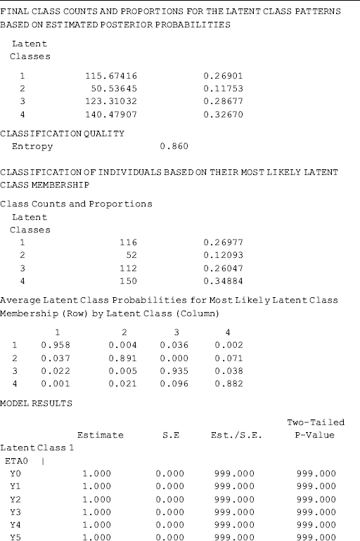
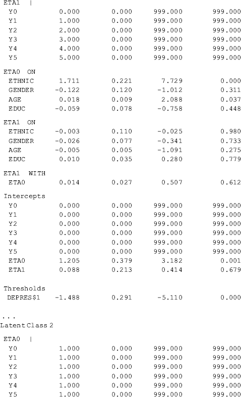
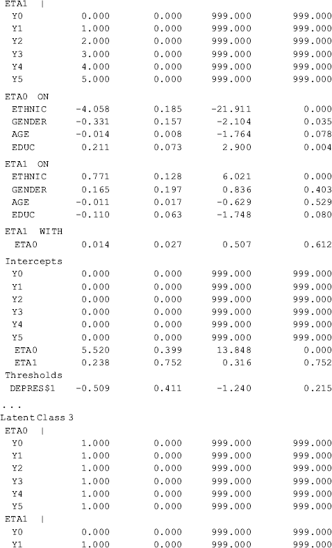
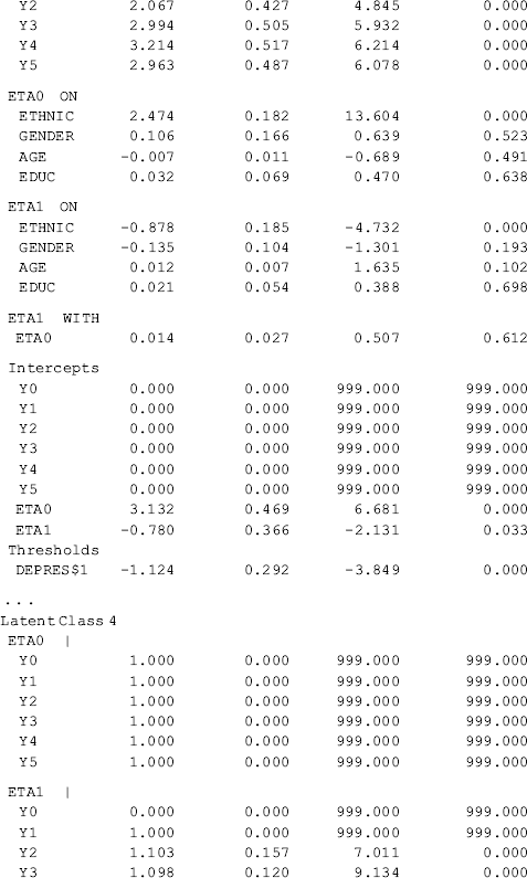
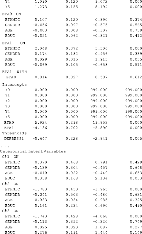
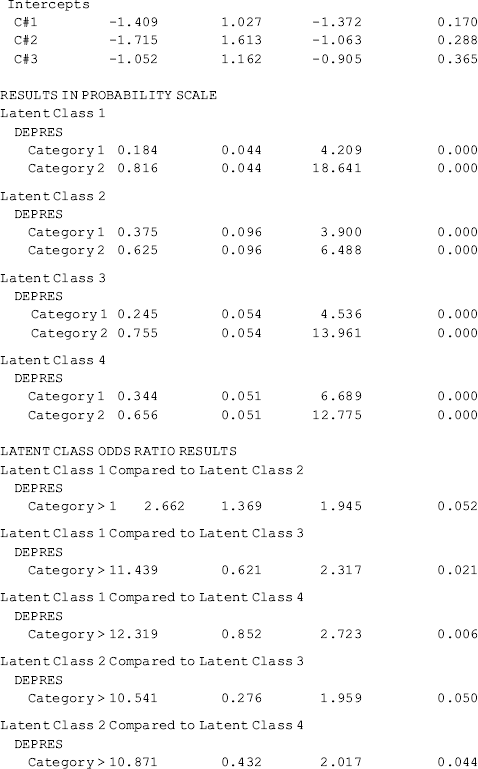
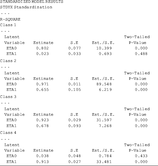
Compared with the unconditional GMM, additional parameter estimates are reported in Table 6.19 for the conditional GMM: (1) the effects of covariates (i.e., Ethnic, Gender, Age, and Educ in this example) on the latent growth factors (i.e., eta0, eta1) in each class; (2) the effects of covariates on latent class membership; and (3) the relationship between the latent class membership and the distal outcome (i.e., Depres in this example). Because regressions of the latent growth factors on covariates are specified in the overall MODEL command, as well as in class-specific MODEL commands, the effects of the covariates on the latent growth factors are allowed to vary across classes (see the MODEL RESULTS section in Table 6.19). For example, the effects of ethnicity on the rate of outcome change or the latent slope growth factor eta1are: − 0.003 (P = 0.980) in Class 1; 0.771 (P < 0.001) in Class 2; − 0.878 (P < 0.001) in Class 3; and 2.048 (P < 0.001) in Class 4. The class-varying effects of covariates imply that the latent class membership moderates the causal relationships between the covariates and the within-class growth trajectories; in other words, the covariates have interactions with the latent class membership, in regard to their effects on outcome growth trajectories.

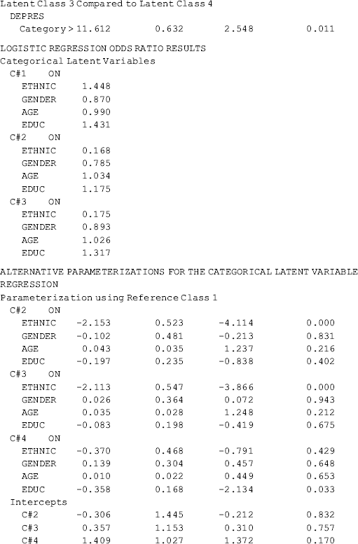
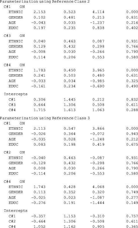
The effects of covariates on latent class membership are estimated by a multinomial logit model and the results are shown in the Categorical Latent Variables section in Table 6.19. With four latent classes, there are three logits in the multinomial logit model where the last class is treated as the reference group. The three sets of regression coefficient estimates are interpreted in the same way as in the regular multinomial logit model. The corresponding odds ratios are reported in the LOGISTIC REGRESSION ODDS RATIO RESULTS section. Additionally, regression coefficient estimates with different latent classes as the reference group are available in the ALTERNATIVE PARAMETERIZATIONS FOR THE CATEGORICAL LATENT VARIABLE REGRESSION section in Table 6.19.

Finally, the relationship between the latent class membership and the distal outcome Depres (0, BDI score ≥ 20); 1, BDI score < 20) is estimated by a binary logistic regression. In Mplus output, there is a threshold estimate for each class that is shown at the bottom of each class-specific section in Table 6.19. For example, the threshold estimates are: DEPRES$1 = −1.488 for Class 1 (P < 0.0001); DEPRES$1 = −0.509 (P = 0.215) for Class 2; DEPRES$1 = −1.124 for Class 3 (P < 0.0001); and DEPRES$1 = −0.647 (P = 0.005) for Class 4. The negative values of these threshold estimates are in fact the intercepts of the logit regression of the distal outcome Depres only on the latent class membership (see Appendix 2.D). The intercept estimates can be used to calculate the probability of having no depression at the end of the 30-month observation period by latent class:

(6.39)

(6.40)

(6.41)

(6.42)

These figures match those reported in the RESULTS IN PROBABILITY SCALE section of Table 6.19. The results show that majority of the crack-cocaine users in each class reported no depression (i.e., BID score <20). However, individuals in Class 1 had the largest probability (0.816), while Class 2 had the lowest probability (0.625), regarding having no depression at the end of the observation period. As to why drug users in Class 1, who used crack-cocaine on daily basis (y0=>4) at baseline and remained at a moderately high level of such drug use over time (see Figure 6.9), had larger likelihood of having no depression needs further study. The relationship between drug use and depression is complicated and beyond the scope of this book.

In this section we have discussed and demonstrated GMM with continuous indicator variables. Other types of indicator variables, such as censored, categorical, count, and combinations of these variable types, can be readily used for GMM (Muthén and Muthén, 1998–2010).

A special case of the GMM is the latent class growth analysis (LCGA) model (Muthén, 2002) or group-based development model (Nagin, 1999, 2005>, >). LCGA identifies distinct growth trajectories and classifies individuals into a finite number of groups, but assuming a homogeneous growth trajectory within each group. Since the GMM is a more generalized model with less restrictive assumptions, the GMM is preferred for mixture modeling with longitudinal data.