4.4 Two-Part LGM
In real research, continuous outcome measures may have a large number of observed values clustered at zero (also known as a semi-continuous outcome measure). Modeling such outcomes has long been a challenge in statistical analysis. Log-transformation cannot solve the problem of extra zeros in the measure, while recoding data into a dichotomous categorical variable (0 vs. 1) for analysis using logistic regression would discard important information. Furthermore, the two-part model developed in econometrics in the early 1980s is often used to analyze data with a concentration of zero values (Duan et al., 1983). This econometric two-part model uses one equation (usually logistic or probit regression) to model the probability of having a nonzero value, and another equation (linear regression) to model the nonzero values, assuming two separate or unconnected models (Manning, Duan, and Rogers, 1987). In most instances, however, the likelihood of having a nonzero value (vs. zero value) and the amount or frequency of nonzero values observed in an outcome are likely to be correlated. By modeling the likelihood and amount separately, the econometric two-part model ignores this correlation, and thus may introduce biases into parameter estimates (Olsen and Schafer, 2001). To deal with this problem, Tooze, Grunwald, and Jones (2002) proposed the Mixed-Effect Mixed Distribution Model and developed a SAS macro program to fit the semi-continuous outcome in longitudinal data. Alternatively, LGM can be readily applied to model the semi-continuous outcome.
In this section we introduce a two-part LGM to model semi-continuous outcome (Olsen and Schafer, 2001; Brown et al., 2005). In such a model, the original distribution of outcome measure is decomposed into two parts: likelihood and amount. These two parts are considered as two associated growth processes and are modeled simultaneously. The data used for model demonstration were collected in a natural history study (N = 249) of stimulant users in rural counties in Western Ohio between October 2002 and September 2004 (Siegal et al., 2006). Frequency of crack-cocaine use in the past 30 days measured at the baseline and every 6 months in the first 2 years of the study period were used as five repeated measures of the outcome. An unconditional two-part LGM is depicted in Figure 4.11.
Figure 4.11 Unconditional two-part LGM.
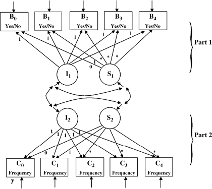
In Part 1 of the model, ‘No use’ of crack-cocaine was separated from the distribution of the observed continuous outcome measure (i.e., number of days crack-cocaine used in the past 30 days), and new binary outcome variables B0, B1, B2, B3, and B4 are created to represent ever used crack-cocaine (1, used crack-cocaine; 0, no use) in the past 30 days prior to each interview. In Part 2 of the model, new continuous outcome variables C0, C1, C2, C3, and C4 are created to represent frequency of crack-cocaine use only among those who had ever used crack-cocaine in the past 30 days. Those who did not use crack-cocaine in the past 30 days were coded as missing cases in the C variables. The LGM with the B variables in the Part 1 model and the LGM with the C variables in the Part 2 model are estimated simultaneously. Associations or causal relationships between the latent growth factors in the two models can be specified based on theory
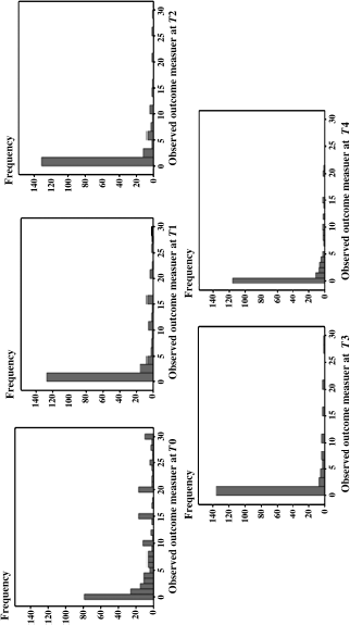
The frequency distributions of the outcome measures are shown in Figure 4.12. As we can see, the outcome measure has a large number of 0 values at each time point, indicating that the repeated outcome measures are semi-continuous variables. As such, the two-part LGM is appropriate for modeling such longitudinal data. The Mplus program for the model follows.
Figure 4.12 Frequency of crack-cocaine use in the past 30 days over time.
Mplus Program 4.14
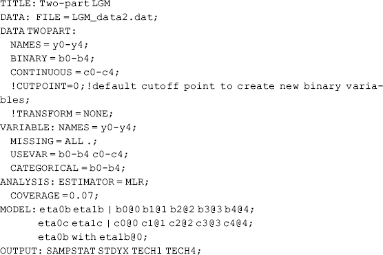
where data were read from a text file named LGM_data2.dat with five repeated measures of crack-cocaine use over time. The DATA TWOPART command is used to create the new binary (B0–B4) and the new continuous (C0–C4) variables from the observed variables (Y0–Y4). If the observed variable is greater than the cut-off point (0 by default), then a new binary variable (i.e., B0–B4) will have a value of 1 (i.e., used crack-cocaine in the past 30 days in this example), otherwise 0 (i.e., no crack-cocaine use in the past 30 days). When the observed variable is not greater than the cut-off point or the new binary variable (i.e., B0–B4) has a value of 0, a missing value will be assigned to the new continuous variable (i.e., C0–C4). If the observed variable has a missing value, a missing value will be assigned to both the new binary and continuous variables. Considering that the new continuous variable may not be normally distributed, Mplus automatically conducts a log transformation of the variable by default, unless the TRANSFORM = NONE option is specified in the DATA TWOPART command.
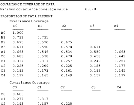
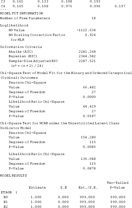
The option COVERAGE = 0.07 on the ANALYSIS command specifies 0.07 or 7% as the minimum acceptable covariance coverage value. When variables involved in the model under study have missing values Mplus provides information on the missing values in the Covariance Coverage Matrix in the Mplus output, in which the diagonal values represent the proportion of nonmissing values for each variable, while the off diagonal values are the proportions of nonmissing values for pairwise combinations of variables. Table 4.14 shows in our example sample only 7.6% of the cases have valid values for the new variables C2 and C4 that are created in Mplus Program 4.14. The explanations for such a low nonmissing value are: 81 participants in the sample did not come back for the 12-month follow-up interview; and among those who had the follow-up interview, 112 of them reported no use of crack-cocaine in the last 30 days prior to T2. As such, the percentage of missing value in the new variable C2 is very high [(81 + 112)/249) = 77.5%] (recall, nonuse of crack-cocaine was coded as missing in the C variables in the model), corresponding to the nonmissing value of 0.225 (22.5%) on the diagonal of the Covariance Coverage Matrix in Table 4.14. For the new variable C4, the nonmissing value is 0.197 (19.7%). For the pairwise combination of C2 and C4, the covariance coverage value is very low (0.076 or 7.6%), that is, less than the minimum acceptable missing value (0.10) set up in Mplus by default. If we did not specify a minimum acceptable missing value in the COVERAGE option of the ANALYSIS command that is less than 0.076, Mplus would print a warning message such as:

For the purpose of model demonstration, we specify COVERAGE = 0.07 in Mplus Program 4.14.
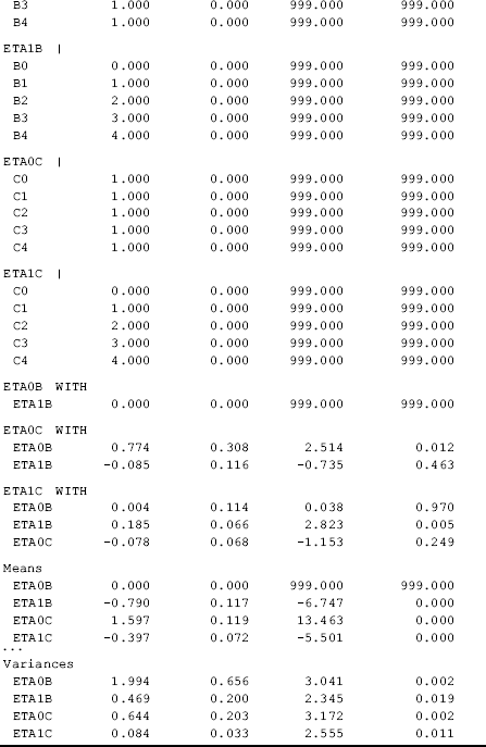
Table 4.14 Selected Mplus output: two-part LGM.
Two-part modeling requires ML estimation. In this example, the robust ML estimator MLR is applied. In the MODEL command, the first ‘|’ statement specifies a linear growth model for the binary outcome (B0–B4), and the second ‘|’ statement specifies a linear growth model for the continuous outcome (C0–C4). For the purpose of model identification, some restrictions are imposed by default: (1) the thresholds of the binary outcome measures are held equal over time to ensure measurement metric invariance; and (2) the mean of the latent intercept growth factor of the binary outcome measure in the Part 1 model is fixed at zero. In our exploratory modeling, the following warning is shown:

In order to prevent the latent variable covariance matrix (PSI) from being non positive definite, the covariance between the growth factors eta0b and eta1b is fixed at 0 by specifying eta0b with eta1b@0 in the MODEL command in Mplus Program 4.14.
The parameter estimates of the two-part LGM are interpreted in the same way as in the LGM models discussed in previous sections. Recall that the Part 1 model in our example is to model the odds of using crack-cocaine in the past 30 days prior to an interview; and the Part 2 model is to model the frequency of crack-cocaine use among those who used crack-cocaine in the past 30 days. Significance of the slope growth factor eta1b (−0.790, P < 0.001) indicates that the odds of using crack in the past 30 days significantly declined over time. In addition, the frequency of crack-cocaine use among those who reported using crack-cocaine also significantly declined (eta1c = −0.397, P < 0.001) (Table 4.14).
For the two-part LGM, Mplus does not provides the familiar model fit indices such as the RMSEA, CFI, TLI, and SRMR. Instead, Table 4.14 only shows the log-likelihood and information criteria for the overall model that can be used for model comparisons. Mplus also provides both the Pearson χ2 and the LR χ2 tests for the binary outcome measures. These two χ2 statistics are supposed to agree with each other; otherwise neither of them is trustable. These two χ2 statistics in our example are not close to each other, and thus they are not trustable.
Other two χ2 statistics in the Mplus output are to test whether data are MCAR (Little, 1988). A nonsignificant Little's MCAR test indicates that the null hypothesis of MCAR cannot be rejected. However, in this example, the Pearson χ2 and the LR χ2 statistics do not agree with each other; thus neither of the tests is trustable.
