2.3 CFA Model with Non-Normal and Censored Continuous Indicators

In Section 2.2 we have discussed and demonstrated CFA with continuous indicators. The default estimator ML requires multivariate normally distributed data for model estimation. Very often, such an assumption is violated in data for social science studies. Under the condition of non- normality, ML parameter estimates are less likely to be biased; however, when non- normality increases the standard errors of ML parameter estimates and model fit indices tend to be underestimated, and model χ ² statistics would be inflated (Browne, 1982; Satorra, 1992; West, Finch, and Curran, 1995; Finch, West, and MacKinnon, 1997). As such, dealing with non- normality is an important issue in SEM. Non- normal data violates the multivariate normality assumption mainly due to skewness, kurtosis, censoring, outlier and influential cases. In this section, we will discuss and demonstrate how to conduct CFA with non- normal and censored data. We start with testing non- normality.

2.3.1 Testing Non-Normality

Mplus allows data screening for outliers and influential cases by checking the Mahalanobis distance (Rousseeuw and Van Zomeren, 1990), log- likelihood distance influence measure (Cook and Weisberg, 1982), and Cook' s D (Cook, 1977), as well as histograms or scatterplots. However, the current version of Mplus does not provide a case- robust estimator to deal with outliers and influential cases. Once outliers and influential cases are identified, they may be deleted from the data (Muthé n and Muthé n, 1998– 2010). Here we focus on non- normality due to skewness and kurtosis.

Technical option TECH13 in Mplus OUTPUT command can be used to test non- normality. TECH13 needs to be used in conjunction with the CLASSES = C(1) statement in the VARIABLE command and TYPE = MIXTURE statement in the ANALYSIS command. The following Mplus program tests non- normality of the 18 observed indicators (x₁ − x₁₈) of the BSI- 18.

Mplus Program 2.5

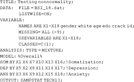
where LISTWISE = ON is required for using TECH13. This program provides two- sided univariate, bivariate, and Mardia multivariate skewness and kurtosis tests (Mardia, 1974; Mardia, Kent, and Bibby, 1979). The test results are basically identical to those estimated from the SAS macro MULTNORM.SAS that can be downloaded free from http://www.dms.umontreal.ca/~bilodeau/stt6515/programme.

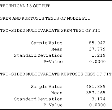
Only multivariate non- normality test results are reported here. If data have a multivariate normal distribution, it implies that each variable in the data has a univariate normal distribution and each pair of variables has a bivariate normal distribution (Hayduk, 1987). The results show that testing for both multivariate skewness and kurtosis are statistically significant (Table 2.4), indicating violation of multivariate normality assumption.

Table 2.4 Selected Mplus output: non-normality test.

2.3.2 CFA Model with Non-Normal Indicators

Some transformations, such as logarithmic transformations, power transformations, square root transformations or logarithmic transformations, are often implemented to deal with non- normal data. Although transformation makes the data more normal looking, interpretation of the model parameter estimates is not straightforward.

Several model- based approaches have been proposed to deal with non- normality and implemented in SEM computer software (West, Finch, and Curran, 1995): (1) ADF estimation method (Browne, 1984); (2) adjusting the normal theory ML χ ² and standard errors using rescaling methods (Satorra and Bentler, 1988); and (3) the bootstrap method (Beran and Srivastava, 1985; Bollen and Stine, 1992, 1993). Because ADF requires large sample size and is computationally demanding, it is not preferred. Though bootstrapping is available in Mplus, it is much more convenient to use the rescaling- based robust estimators in Mplus (e.g., MLR, MLM) to deal with non- normality in data.

Rescaling- based robust estimators, such as the robust MLR estimator and the MLM estimator, are available in Mplus (Muthé n, 1998– 2004; Muthé n and Muthé n, 1998– 2010). MLR provides standard errors and test statistic that are robust to non- normality. MLM provides robust standard errors and mean- adjusted test statistic that are equivalent to Satorra & Bentler (SB) and standard errors produced in EQS (Bentler, 2005). MLM cannot handle missing values in the current version of Mplus. With missing data, MLR is used to obtain robust estimates; it is also recommended for small and medium sample size (Yuan and Bentler, 2000; Muthé n and Asparouhov, 2002). In the following Mplus program we use the MLR estimator to handle non- normality.

Mplus Program 2.6

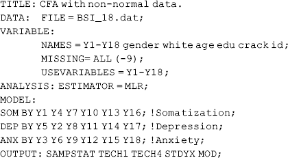
where the default estimator ML is replaced with the robust estimator MLR by specifying ESTIMATOR = MLR on the ANALYSIS command line.

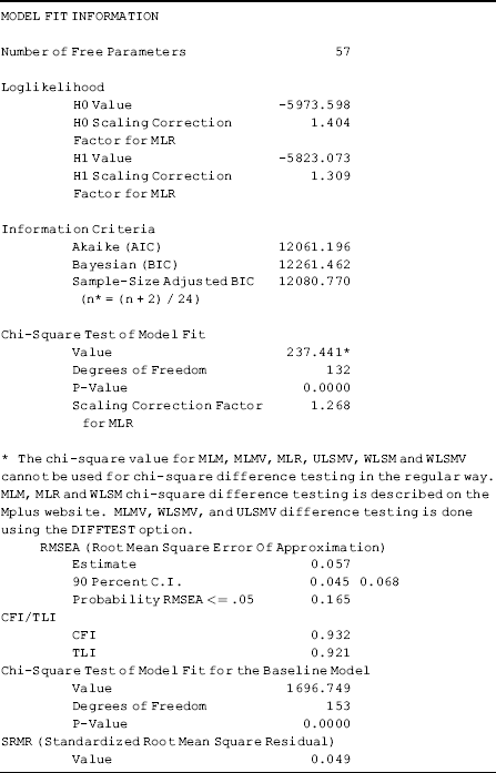
Using the robust estimator MLR, model fits data very well with no error covariance specified: RMSEA = 0.057 (90% CI: 0.045; 0.068), close- test P- value = 0.165, CFI = 0.932, TLI = 0.921, and SRMR = 0.049 (Table 2.5).

Table 2.5 Selected Mplus output: CFA using robust estimator MLR.

Using MLM, which is another robust ML estimator, the model results are very close to those shown in Table 2.5. Since MLM estimator does not allow for missing values, it has to be used in conjunction with the LISTWISE = ON statement in the DATA command. As a result, cases with any missing values would be deleted. For example, using MLM for our example model, only 243 cases would be used for modeling.

Since the ML robust estimator is easy to apply and works well under either normality or non- normality conditions, we do not have to test for non- normality before deciding whether a robust estimator should be used. As data normality assumption barely holds in social science studies, it is always safer to use robust estimators for model estimation. The robust estimators MLR is also flexible in dealing with missing values. For MLR, it is not necessary to assume that missingness is MCAR, but a much less restrictive assumption of MAR can be assumed. With MAR, missingness is allowed to be related to both the observed covariates and outcomes. This is very important for data analysis, particularly for longitudinal studies. MAR allows attrition to be related to baseline outcome level, individual characteristics, and intervention/treatment assignment. In contrast, the robust WLS estimators (e.g., WLSMV, WLSM,..) allow missingness to be a function of the observed covariates but not the observed outcomes; therefore, missingness allowed for WLS estimators is less restrictive than MCAR, but more restrictive than MAR. Note that MLM cannot deal with missing values.

Note that when a robust estimator is used for model estimation, the Mplus output alerts that model statistics estimated from the robust estimators cannot be directly used for the LR test because the difference between two model s for nested models does not follow a distribution (Muthé n and Muthé n, 1998– 2010). When estimators, such as MLM, MLR or WLSM, are used for model estimation, a scaled difference in s should be computed for nested model comparison (http://www.statmodel.com/chidiff.shtml). When MLMV, WLSMV or ULSMV is used for model estimation, a two- stage approach is available in Mplus for difference testing.

In the following Mplus program, the CFA model is rerun with equality restrictions on the factor loadings to each factor; and a LR test will be conducted to test whether the indicators of each factor are equally loaded to the underlying factor.

Mplus Program 2.7

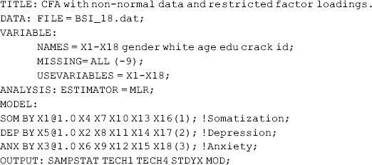
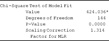
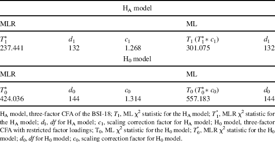
where the labels (1), (2), and (3) in the BY statements of the MODEL command constrain the factor loadings on each factor to be equal. With these restrictions, the number of free parameters will reduce by 3^* (5 − 1) = 12. Namely, the df of the model will increase by 12 from 132 to 144; and the MLR statistic increased from 237.441 to 424.036 (cf. Tables 2.5 and 2.6). Following the steps to compare two nested models estimated from a robust estimator (e.g., MLR, MLM, or WLSM) as described in the Mplus website (http://www.statmodel.com/chidiff.shtml), we can calculate the scaled difference in s for model comparison.

Table 2.6 Selected Mplus output for the restricted model.

(2.6)

where TR_d is the scaled difference in s, T₀ is the ML statistic for the H₀ model, T₁ is the ML statistic¹¹ for the H₁ model, and c_d is the difference test scaling correction.

(2.7)

where d₀ and c₀ are the df and the scaling correction factor for the H₀ model, and d₁ and c₁ are the df and the scaling correction factor for the H₁ model (Table 2.7). Substituting the corresponding values in Table 2.7 into Equations (2.6) and (2.7), we have

(2.8)

For this test, df = 144 − 132 = 12. The test is statistically significant (P < 0.001) at the 0.05 level.¹² Thus, we conclude that restricting factor loadings makes model fit significantly worse. In other words, the BSI- 18 items do not have identical factor loadings on their underlying factors.

Table 2.7 Calculating scaled difference in χ² test for nested model comparison using robust estimator.

2.3.3 CFA Model with Censored Data

Censored data are usually defined as a censored normal distribution. In social science studies, some outcomes measures are often censored. For example, when exam questions are not sufficiently difficult, thus a substantial number of students receive the total possible score, and there is no variation among the ‘ top’ students. This is called high- end censoring or above censoring. Another example is the amount of money that people spend on expensive durable goods (e.g., computer, piano, car, etc.) in a given period (e.g., a year). Among people who spend nothing on high- end durables, some of them may never buy any high- end durables (they have a real zero value), while some of them might be ready to buy, but have not done so yet. Irrespective of the underlying propensity of those individuals, the observed outcome values are ‘ zero’ for those who do not buy any high- end durables in the study period. In this case, censoring arises on the low end or the minimum of the scale – this is so- called below censoring. Of course, censoring could occur at both the low and high ends. For example, Likert scales typically provide a limited number of ordinal responses for an underlying continuous variable. For example, self- reported health status may be measured on a five- point scale: 1, very bad; 2, bad; 3, do nott know; 4, good; and 5, very good. Under some circumstances, responses might ‘ pile up’ at both ends of the spectrum of the health scale. Censoring also often comes with the way questions are asked in surveys. For example, a survey may have some lower and upper limits in its questions such as income ≤ US$ 10,000 and income ≥ US$ 100,000. In this case, censoring occurs at both the low and high ends.

When an outcome measure is censored, its distribution is distorted. Regression models that ignore the presence of censoring can produce biased coefficient estimates. The classical TOBIT regression model (Tobin, 1958; Greene, 1990) is usually used for modeling an underlying normal (uncensored) outcome measure that is censored from below or above at a known point. Mplus has the capacity of conducting the TOBIT model with above censoring only, below censoring only or both. The following Mplus program is to check the frequencies of the observed variables.

Mplus Program 2.8

where the PLOT command allows us to use the plot generator in Mplus. The statement TYPE = PLOT1 tells Mplus to create plots for observed variables. After running the program, you can view plots of the variable by clicking on Graph → View Graphs → Histograms (sample values) → View → Select Variables → OK. Mplus also allows you to export the plots with different image formats. For example, once a plot is shown on screen, you can click on Graph → Export Plot to → JPEG, then save it as a JPEG image file in your selected folder.

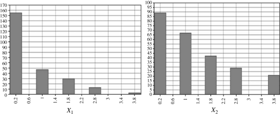
Figure 2.3 shows the frequencies of the selected indicators from the BSI- 18 data set. For both X₁ and X₂ observed values pile up at the lower end of the five- point Likert scale (0, not at all; 1, a little bit; 2, moderately; 3, quite a bit; 4, extremely).

Figure 2.3 Frequencies of selected indicators (X₁ and X₂).

For the purpose of demonstration, we treat indicators X₁ and X₂ as measures with below censoring in the following Mplus program.

Mplus Program 2.9

where x₁ and x₂ are specified as indicators with below censoring by adding the statement CENSORED = X1 X2 (b) in the VARIABLE command. When indicators are specified as censored measures, model estimation will be very time- consuming. In addition, the current version of Mplus only provides log- likelihood values and information criteria, but no model fit indices (e.g., CFI, TLI, RMSEA, SRMR, WRMR) and MIs.

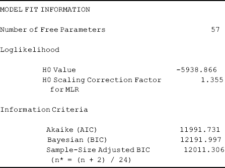
The model estimation terminated normally, and the model results show smaller log- likelihood values and smaller information criteria (Table 2.8), compared with those estimated from the CFA model without taking into account censoring.

The above model example demonstrates how to conduct CFA with censored indicators. Interested readers may try to determine how to run the traditional TOBIT model in Mplus (i.e., regressing an observed censored dependent on observed independent variables).

Table 2.8 Selected Mplus output: CFA with censored continuous indicators.