6.4 Factor Mixture Model

The GMM for longitudinal data analysis discussed in the previous section is a hybrid model that involves both continuous latent variables (i.e., the latent growth factors) and the categorical latent variable (the latent class variable). An example of cross-sectional hybrid model is the factor mixture analysis (FMA) model, which is a hybrid model of the factor analysis model (either EFA or CFA) and latent class model (Lubke and Muthén, 2005; Muthén, 2006; Muthén and Asparouhov, 2006). In a FMA, the factor analysis model clusters items on factors (continuous latent variables) and generates factor scores; and the LCA model clusters individuals/cases into groups (latent categorical variable) with different factor mean scores (Lubke and Muthén, 2005, 2007>, >). Thus, like the GMM, the FMM is a combination of a variable-centered and person-centered modeling approach.

According to Muthèn (2008), hybrid latent variable models can be categorized into four branches. The first two assume measurement invariance, while the last two assume measurement noninvariance, across classes (Muthén, 2008). In this section, we discuss on FMA models that belong to the first two branches: (1) FMA with measurement invariance and parametric factor distribution, also called mixture factor analysis (MFA); and (2) FMA with measurement invariance and nonparametric factor distribution, also called nonparametric factor analysis or latent class factor analysis (LCFA) (Muthén, 2008). The MFA model can be described as:

(6.43)

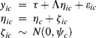
where the measurement parameters (e.g., factor loadings and indicator/item intercepts) are restricted equal across classes,¹⁴ and the factor variances and covariances are set as free parameters. In the model, the within-class item covariances are described by a CFA model and the factorial structure of the CFA model remains the same across classes; and individuals are clustered into different classes, each of which has different factor mean(s) and variance(s)/covariance(s). If we impose equality restriction on within-class factor scores (i.e., set within factor variance to 0, resulting in = 0, thus ) in Equation (6.43), then the MFA model becomes the LCFA model, in which there is no variation in factor scores within each class, but factor means are varying across classes.

The MFA and LCFA models with three latent classes are depicted in Figure 6.10a and b, respectively. The only difference in the model diagrams between the MFA and the LCFA is that the former allows a parametric factor distribution, usually assuming a normal distribution with zero means and variances (), for each class (see the right-hand side of Figure 6.10a), while the latter only estimates factor mean for each class with nonparametric distribution (on the right-hand side of Figure 6.10b, instead of parametric distribution, latent classes are represented by bars marking the factor means). On the left-hand side of Figure 6.10a there is an arrow pointing to factor in the MFA model, indicating within-class factor score variation, while the LCFA model has no such arrow (see the left-hand side of Figure 6.10b) because it assumes no within-class variation.

Figure 6.10 (a) MFA model; (b) nonparametric factor analysis model – LCFA.

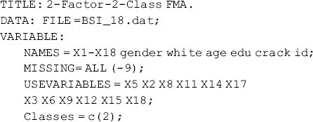
In the following, an example of a MFA model is demonstrated using the data set BSI-18.dat that was used for model demonstrations in Chapter 2. The within-class model of the MFA is a two-factor (Depression and Anxiety) CFA model; and the LCA part of the MFA classifies individuals into classes with different levels of factor means. Before we run the MFA, we first test the two-factor CFA model,¹⁵ and the results show that the model fits data very well (RMSEA = 0.056, 90% CI (0.036, 0.074), close-fit test P-value = 0.297; CFI = 0.961; TLI = 0.950; and SRMR = 0.043). After the measurement model has been confirmed, we then explore the possible unobserved population heterogeneity, in regard to factor scores of Depression and Anxiety. A 2-factor, 2-class model with measurement invariance is compared with the single class model, and the 2-class model fits data better with smaller AIC, BIC, and ABIC. Though the P-values of the LMR LR and ALMR LR tests are >0.05, the P-value of BLRT is < 0.001. The results provide evidence of unobserved population heterogeneity. As for other mixture models, to determine the finite number of the unobserved subpopulations, we need to run FMA models with an increasing number of classes and compare their model fit indices and statistics. In our example, the model estimation of the 2-factor, 3-class model did not terminate normally; therefore, the 2-factor, 2-class model is chosen for model demonstration. The corresponding Mplus program follows:

Mplus Program 6.10

where measurement parameters (item intercepts, factor loadings, and error variances), as well as the error term covariance between items x₈ and x₅, are set invariant across classes by default. In addition, the factor variances/covariances are free parameters, but are restricted to be invariant across classes by default. To reduce the computing time, we first fit the model without TECH14, and then the seed 79945 that was associated with the best log-likelihood value was specified in the OPTSEED statement of the ANALYSIS command in the Mplus Program 6.10.

Selected model results are shown in Table 6.20. Among the 248 cases in the sample, 41 (16.5%) were classified into Class 1, and the rest into Class 2. The latent class classification is adequate. Correct class membership classification counts are about 93.4% for Class 1 and 98.1% for Class 2; and entropy = 0.897, which is much higher than the cut-off point of 0.70 (Nagin, 2005).

Table 6.20 Selected Mplus output: 2-factor, 2-class MFA model.

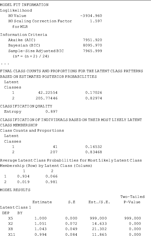
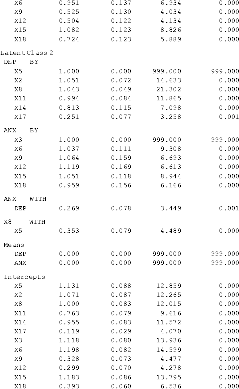
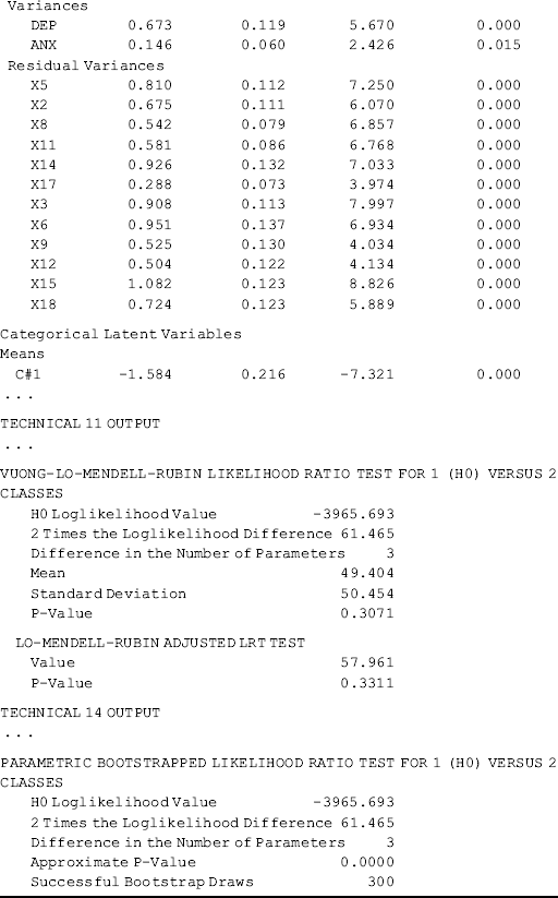
The key interest of the model is the factor mean differences between the latent classes. As usual, the last class is treated as the reference group, for which all factor mean estimates are 0 for the purpose of model identification (Chapter 5) (e.g., the mean values of both factors DEP and ANX are 0 for Class 2 in Table 6.20). Mplus output shows that the estimated factor ‘means’ of DEP and ANX for Class 1 are 1.270 and 1.816, respectively. As a matter of fact, these figures are not the means of factors DEP and ANX; instead they are the factor mean differences between Classes 1 and 2, indicating that the levels of depression and anxiety are higher among individuals in Class 1 than those in Class 2.

In the Categorical Latent Variables section in Table 6.20, we see Means C#1 = −1.584. This number is not a mean, but the log odds of being classified in Class 1. It can be converted to a probability of exp(−1.584)/[exp(−1.584) + 1] = 0.170 that matches the figure shown in the FINAL CLASS COUNTS AND PROPORTIONS FOR THE LATENT CLASS PATTERNS BASED ON ESTIMATED POSTERIOR PROBABILITIES section in Table 6.20.

Covariates can be readily included in the model to predict factors; as such, the MFA is expanded to a mixture MIMIC model; by replacing the factor covariances with causal relationships between factors, the MFA model becomes a mixture SEM model. For example, the following Mplus program estimates a simple mixture SEM model, in which covariate Gender predicts the factors ANX and DEP, while ANX predicts factor DEP within each latent class.

Mplus Program 6.11

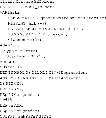
where the regressions are specified in both the overall MODEL and class-specific MODEL commands; thus the regression coefficients are allowed to vary across classes. By comparing the model χ² statistics of this model with the model χ² statistics where equality restrictions are imposed on the regression coefficients, we will be able to test causal effect invariance across the latent classes.

The model results show that Gender has a significant negative effect (−0.921, P = 0.001) on ANX only in Class 1 (i.e., the class with higher depression and anxiety levels) (Mplus output is not reported here). Again, inclusion of covariates in the model changes latent class classification to some extent. This is just like the situation where covariates are included in a LCA model or GMM.

LCFA model. As aforementioned, LCFA is a special case of MFA. By fixing the within-class factor variances to 0, the MFA model becomes a LCFA model (the model is not demonstrated here). The model results of the LCFA model are interpreted similarly to those of the FMA model. However, covariates cannot be included to predict factors, though they can be included to predict the latent class membership, because there is no within-class factor score variation in such a model.

In this chapter we have discussed and demonstrated some fundamental mixture models for both cross-sectional and longitudinal data analyses. Mixture models are a useful statistical approach to explore and analyze unobserved population heterogeneity. Although such models have not yet been widely applied in real research, they are increasingly gaining in popularity. Additionally, mixture modeling has been recently been incorporated in multilevel modeling, thus establishing a more generalized modeling framework. Interested readers are referred to Asparouhov and Muthen (2008) and Muthén and Asparouhov (2011c).