
1.1 Model Formulation
In SEM, researchers begin with the specification of a model to be estimated. There are different approaches to specify a model of interest. The most intuitive way of doing this is to describe one's model by path diagrams first suggested by Wright (1934). Path diagrams are fundamental to SEM since it allows researchers to formulate the model of interest in a direct and appealing fashion. The diagram provides a useful guide for clarifying a researcher's ideas about the relationships among variables and they can be directly translated into corresponding equations for modeling. Several conventions are used in developing a SEM model path diagram, in which the observed variables (also known as measured variables, manifest variables, or indicators) are presented in boxes, and latent variables or factors are in circles or ovals. Relationships between variables are indicated by lines; lack of line connecting variables implies that no direct relationship has been hypothesized between the corresponding variables. A line with a single arrow represents a hypothesized direct relationship between two variables, with the head of the arrow pointing toward the variable being influenced by another variable. The bidirectional arrows refer to relationships or associations, instead of effects, between variables.
An example of a hypothesized general structural equation model is specified in the path diagram shown in Figure 1.1. As mentioned above, the latent variables are enclosed in ovals and the observed variables are in boxes in the path diagram. The measurement of a latent variable or a factor is accomplished through one or more observable indicators, such as responses to questionnaire items that are assumed to represent the latent variable. In our example two observed variables (x1 and x2) are used as indicators of the latent variable ξ1, three indicators (x1 − x3) for latent variable ξ2, and three (y1 − y3) for latent variable η1. Note that η2 has a single indicator, indicating that the latent variable is directly measured by a single observed variable. This special case will be discussed later.
Figure 1.1 A hypothesized general structural equation model.
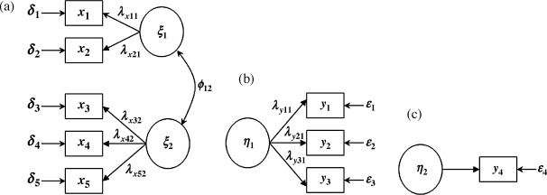
The latent variables or factors that are determined by variables within the model are called endogenous latent variables, denoted by η; the latent variables, whose causes lie outside the model, are called exogenous latent variables, denoted by ξ. In the example model, there are two exogenous latent variables (ξ1 and ξ2) and two endogenous latent variables (η1 and η2). Indicators of the exogenous latent variables are called exogenous indicators (e.g., x1 − x5), and indicators of the endogenous latent variables are endogenous indicators (e.g., y1 − y4). The former has a measurement error term symbolized as δ, and the latter has measurement errors symbolized as ε (Figure 1.1).
The coefficients ![]() and
and ![]() in the path diagram are path coefficients. The first subscript notation of a path coefficient indexes the dependent endogenous variable, and the second subscript notation indexes the causal variable (either endogenous or exogenous). If the causal variable is exogenous (ξ), the path coefficient is a γ; if the causal variable is another endogenous variable (η), the path coefficient is a β. For example, β12 is the effect of endogenous variable η2 on the endogenous variable η1; γ12 is the effect of the second exogenous variable ξ2 on the first endogenous variable η1. As in multiple regressions, nothing is predicted perfectly; there are always residuals or errors. The ζs in the model, pointing toward the endogenous variables, are structural equation residual terms.
in the path diagram are path coefficients. The first subscript notation of a path coefficient indexes the dependent endogenous variable, and the second subscript notation indexes the causal variable (either endogenous or exogenous). If the causal variable is exogenous (ξ), the path coefficient is a γ; if the causal variable is another endogenous variable (η), the path coefficient is a β. For example, β12 is the effect of endogenous variable η2 on the endogenous variable η1; γ12 is the effect of the second exogenous variable ξ2 on the first endogenous variable η1. As in multiple regressions, nothing is predicted perfectly; there are always residuals or errors. The ζs in the model, pointing toward the endogenous variables, are structural equation residual terms.
Different from the traditional statistical methods, such as multiple regressions, ANOVA, and path analysis, SEM focuses on latent variables/factors rather than on the observed variables. The basic objectives of SEM are to provide a means of estimating the structural relations among the unobserved latent variables of a hypothesized model free of the effects of measurement errors. These objectives are fulfilled through integrating a measurement model (confirmatory factor analysis, CFA) and structural model (structural equations or latent variable model) into the framework of a structural equation model. It can be claimed that a general structural equation model consists of two parts: (1) the measurement model that links observed variables to unobserved latent variables (factors); and (2) structural equations that link the latent variables to each other via a system of simultaneous equations (Jöreskog, 1973).
1.1.1 Measurement Model
A measurement model is the measurement component of a structural equation model. The main purpose of a measurement model is to describe how well the observed indicator variables serve as a measurement instrument for the underlying latent variables or factors. Measurement models are usually carried out and evaluated by CFA. As a measurement model, CFA proposes links or relations between the observed indicator variables and the underlying latent variables/factors that they are designed to measure; then, it tests them against the data to ‘confirm’ the proposed factorial structure.
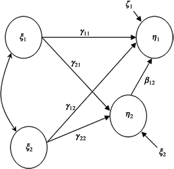
In the structural equation model specified in Figure 1.1, three measurement models can be considered (Figure 1.2a–c). In each measurement model, the λ coefficients, which are called factor loadings in the terminology of factor analysis, are the links between the observed variables and latent variables. For example, in Figure 1.2a the observed variables x1 − x5 are linked through ![]() to latent variables ξ1 and ξ2, respectively. In Figure 1.2b the observed variables y1 − y3 are linked through
to latent variables ξ1 and ξ2, respectively. In Figure 1.2b the observed variables y1 − y3 are linked through ![]() to latent variable η1. Note that Figure 1.2c can be considered as a special CFA model with a single factor η2 and a single indicator y4. Of course this model cannot be estimated separately because it is unidentified. We will discuss this issue later.
to latent variable η1. Note that Figure 1.2c can be considered as a special CFA model with a single factor η2 and a single indicator y4. Of course this model cannot be estimated separately because it is unidentified. We will discuss this issue later.
Figure 1.2 (a) Measurement model 1. (b) Measurement model 2. (c) Measurement model 3.

Factor loadings in CFA models are usually denoted by the Greek letter ![]() . The first subscript notation of a factor loading indexes the indicator, and the second subscript notation indexes the corresponding latent variable. For example,
. The first subscript notation of a factor loading indexes the indicator, and the second subscript notation indexes the corresponding latent variable. For example, ![]() represents the factor loading linking indicator x2 to exogenous latent variable ξ1; and
represents the factor loading linking indicator x2 to exogenous latent variable ξ1; and ![]() represents the factor loading linking indicator y3 to endogenous latent variable
represents the factor loading linking indicator y3 to endogenous latent variable ![]() .
.
In the measurement model shown in Figure 1.2a, there are two latent variables/factors, ξ1 and ξ2, each of which is measured by a set of observed indicators. Observed variables x1 and x2, are indicators of the latent variable ξ1, and x3 − x5 are indicators of ξ2. The two latent variables, ξ1 and ξ2, in this measurement mode are correlated with each other (ϕ12 in Figure 1.2a stands for the covariance between ξ1 and ξ2), but no directional or causal relationship is assumed between the two latent variables. If these two latent variables were not correlated with each other (i.e., ϕ12 = 0) there would be a separate measurement model for ξ1 and ξ2, respectively, where the measurement model for ξ1 would have only two observed indicators, thus it would not be identified.
For a one-factor solution CFA model, a minimum of three indicators is required for model identification. If no errors are correlated, a one-factor CFA model with three indicators (e.g., the measurement model shown in Figure 1.2b) is just identified (i.e., the number of observed variances/covariances equals the number of free parameters).1 In such a case, model fit cannot be assessed although model parameters can be estimated. In order to assess model fit, the model must be over-identified (i.e., the observed pieces of information are more than model parameters that need to be estimated). Without specifying error covariances, a one-factor solution CFA model needs at least four indicators in order to be over-identified. However, a factor with only two indicators may be acceptable if the factor is specified to be correlated with at least one of the other factors in a CFA model and no error terms are correlated with each other (Bollen, 1989a; Brown, 2006). The measurement model shown in Figure 1.2a is over-identified though factor ξ1 has only two indicators. Nonetheless, multiple indicators need to be considered to represent the underlying construct more completely since different indicators can reflect nonoverlapping aspects of the underlying construct.
Figure 1.2c shows a simple measurement model. For some single observed indicator variables (e.g., gender, ethnicity) that are less likely to have measurement errors, the simple measurement model would become like y4 = η2, where factor loading λy42 is set to 1.0 and measurement error ε4 is 0.0. That is, the observed variable y4 is a ‘perfect’ measure of construct η2. If the single indicator is not a perfect measure, measurement error cannot be modeled but rather one must specify a fixed measurement error variance based on a known reliability of the indicator (Hayduk, 1987; Wang et al., 1995). This issue will be discussed in Chapter 3.
1.1.2 Structural Model
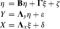
Once latent variables/factors have been assessed in the measurement models, the potential relationships among the latent variables are hypothesized and assessed in the structural model (structural equations or latent variable model) (Figure 1.3), in which path coefficients γ11, γ12, γ21, and γ22 specify the effects of the exogenous latent variables ξ1 and ξ2 on the endogenous latent variables η1 and η2, while β12 specifies the effect of η2 on η1; that is, the structural model defines the relationships among the latent variables, and it is estimated simultaneously with the measurement models. Note, if the variables in a structural model were all observed variables, rather than latent variables, the structural model would become a modeling system of structural relationships among a set of observed variables; thus, the model reduces to the traditional path analysis in sociology or simultaneous equation model in econometrics.
Figure 1.3 Structural model.
The model shown in Figure 1.3 is a recursive model. If the model allows for reciprocal or feedback effects (e.g., η1 and η2 influence each other), then the model is called a nonrecursive model. Applications of only recursive models will be discussed in this book. Readers who are interested in nonrecursive models are referred to Berry (1984) and Bollen (1989a).
1.1.3 Model Formulation in Equations
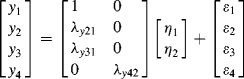
When the covariance structure is analyzed, the general structural equation model can be expressed by three basic equations:
These three equations are expressed in matrix format. Definitions of the variable matrices involved in the three equations are shown in Table 1.1.
Table 1.1 Definitions of the variable matrices in the three basic equations of the general structural equation model.
| Variable | Definition | Dimension |
| η (eta) | Latent endogenous variable | m × 1 |
| ξ (xi) | Latent exogenous variable | n × 1 |
| ζ (zeta) | Residual term in equations | m × 1 |
| y | Endogenous indicators | p × 1 |
| x | Exogenous indicators | q × 1 |
| ε (epsilon) | Measurement errors of y | p × 1 |
| δ (delta) | Measurement errors of x | q × 1 |
| Note: m and n represent the number of latent endogenous and exogenous latent variables, respectively; p and q are the number of endogenous and exogenous indicators, respectively, in the sample. | ||
The first equation in Equation (1.1) represents the structural model which establishes the relationships or structural equations among latent variables. The components of ![]() are endogenous latent variables; and the components of
are endogenous latent variables; and the components of ![]() are exogenous latent variables. The endogenous and exogenous latent variables are connected by a system of linear equations with coefficient matrices
are exogenous latent variables. The endogenous and exogenous latent variables are connected by a system of linear equations with coefficient matrices ![]() (beta) and
(beta) and ![]() (gamma), as well as a residual vector
(gamma), as well as a residual vector ![]() (zeta), where
(zeta), where ![]() represents effects of exogenous latent variables on endogenous latent variables,
represents effects of exogenous latent variables on endogenous latent variables, ![]() represents effects of some endogenous latent variables on other endogenous latent variables, and
represents effects of some endogenous latent variables on other endogenous latent variables, and ![]() represents the regression residual terms.
represents the regression residual terms.
The second and third equations in Equation (1.1) represent measurement models which define the latent variables from the observed variables. The second equation links the endogenous indicators – the observed y variables – to endogenous latent variables (i.e., ηs), while the third equation links the exogenous indicators – the observed x variables – to the exogenous latent variables (i.e., ξs). The observed variables y and x are related to the corresponding latent variables η and ξ by factor loadings ![]() y (lambda y) and
y (lambda y) and ![]() x. The ε and δ are the measurement errors associated with the observed variables y and x, respectively. It is assumed that E(ε) = 0, E(δ) = 0, Cov (ε, ξ) = 0, Cov (ε, η) = 0, Cov (δ, η) = 0, Cov (δ, ξ) = 0, and Cov (ε, δ) = 0, but Cov(εi, εj) and Cov (ηi, ηj) (i ≠ j) might not be zero.
x. The ε and δ are the measurement errors associated with the observed variables y and x, respectively. It is assumed that E(ε) = 0, E(δ) = 0, Cov (ε, ξ) = 0, Cov (ε, η) = 0, Cov (δ, η) = 0, Cov (δ, ξ) = 0, and Cov (ε, δ) = 0, but Cov(εi, εj) and Cov (ηi, ηj) (i ≠ j) might not be zero.
Note that no intercepts are specified in the above SEM equations. This is because the deviations from means of the original observed variables are usually used in structural equation model specification for simplicity. The original observed variables will be used for model estimation when estimates of intercepts, the means, and thresholds of variables are involved in a model. We will discuss this issue in later chapters on modeling categorical outcomes and multi-group modeling.
In the three basic equations shown in Equation (1.1), there are a total of eight parameter matrices in LISREL notation:2 ![]() x,
x, ![]() y,
y, ![]() ,
, ![]() ,
, ![]() ,
,![]() ,
, ![]() and
and ![]() (Jöreskog and Sörbom, 1981). A SEM model is fully defined by the specification of the structure of the eight matrices. In the early stages of SEM, a SEM model was specified in matrix format using the eight-parameter matrix. Although this is no longer the case in current SEM programs/software, information about parameter estimates in the parameter matrices are reported in the output of Mplus and other SEM computer programs. Understanding these notations is helpful for researchers to check the estimates of specific parameters in the output.
(Jöreskog and Sörbom, 1981). A SEM model is fully defined by the specification of the structure of the eight matrices. In the early stages of SEM, a SEM model was specified in matrix format using the eight-parameter matrix. Although this is no longer the case in current SEM programs/software, information about parameter estimates in the parameter matrices are reported in the output of Mplus and other SEM computer programs. Understanding these notations is helpful for researchers to check the estimates of specific parameters in the output.
A summary of these matrices is presented in Table 1.2. The first two matrices, ![]() and
and ![]() , are factor loading matrices that link the observed indicators to latent variables η and ξ, respectively. The next two matrices,
, are factor loading matrices that link the observed indicators to latent variables η and ξ, respectively. The next two matrices, ![]() (beta) and Γ (gamma), are structural coefficient matrices. The
(beta) and Γ (gamma), are structural coefficient matrices. The ![]() matrix is an m × m coefficient matrix representing the relationships among latent endogenous variables. The model assumes that (I −
matrix is an m × m coefficient matrix representing the relationships among latent endogenous variables. The model assumes that (I − ![]() ) must be nonsingular, thus, (I −
) must be nonsingular, thus, (I − ![]() )−1 exists so that model estimation can be done. A zero in the
)−1 exists so that model estimation can be done. A zero in the ![]() matrix indicates the absence of an effect of one latent endogenous variable on another. For example, η12 = 0 indicates that the latent variable η2 does not have an effect on η1. Note that the main diagonal of matrix
matrix indicates the absence of an effect of one latent endogenous variable on another. For example, η12 = 0 indicates that the latent variable η2 does not have an effect on η1. Note that the main diagonal of matrix ![]() is always zero; that is, a latent variable η cannot be a predictor of itself. The Γ matrix is an m × n coefficient matrix that relates latent exogenous variables to latent endogenous variables.
is always zero; that is, a latent variable η cannot be a predictor of itself. The Γ matrix is an m × n coefficient matrix that relates latent exogenous variables to latent endogenous variables.
Table 1.2 Eight fundamental parameter matrices for the general structural equation model.
| Matrix | Definition | Dimension |
| Coefficient matrices | ||
| Factor loadings relating y to η | p × m | |
| Factor loadings relating x to ξ | q × n | |
| Coefficient matrix relating η to η | m × m | |
| Γ (gamma) | Coefficient matrix relating ξ to η | m × n |
| Variance/covariance matrices | ||
| Φ (phi) | Variance/covariance matrices of ξ | n × n |
| Ψ (psi) | Variance/covariance matrices of ζ | m × m |
| Θε (theta-epsilon) | Variance/covariance matrices of ε | p × p |
| Θδ (theta-delta) | Variance/covariance matrices of δ | q × q |
| Note: p is the number of y variables, q is the number of x variables, n is the number of ξ variables, and m is the number of η variables. | ||
There are four parameter variance/covariance matrices for a general structural equation model: Φ (phi), Ψ (psi), Θε (theta-epsilon), and Θδ (theta-delta).3 All four variance/covariance matrices are symmetric square matrices; that is, the number of rows equals the number of columns in each of the matrices. The elements in the main diagonal of each of the matrices are the variances that should always be positive; the elements in the off-diagonal are covariances of all pairs of variables in the matrices. When all the variables, both observed variables (i.e., indicators of latent variables) and latent variables are standardized, each of the variance/covariance matrices would become a correlation matrix in which the diagonal values would all become 1, and the off-diagonal values would become correlations. The n × n matrix Φ is the variance/covariance matrix for the latent exogenous variable ξs. Its off-diagonal element ϕij (i.e., the element in the ith row and jth column in matrix Φ) is the covariance between the latent exogenous variables ξi and ξj (i ≠ i). If ξi and ξj were not hypothesized to be correlated with each other in the model, ϕij = 0 should be set up when specifying the model. The m × m matrix Ψ is the variance/covariance matrix of the residual terms ζ of the structural equations. In simultaneous equations of econometrics, the disturbance terms in different equations are often assumed to be correlated with each other. This kind of correlation can be readily set up in matrix Ψ and estimated in SEM. The last two variance/coviances matrices (i.e., the p × p Θε and q × q Θδ) are variance/covariance matrices of the measurement errors for the observed variables y and x, respectively. In longitudinal studies, the autocorrelations can be easily handled by correlating specific error terms with each other.
SEM model specification is actually to formulate a set of model parameters contained in the eight matrices. Those parameters can be specified as either fixed or free. Fixed parameters are not estimated from the model and their values are typically fixed at zero (e.g., zero covariance or zero slope indicating no relationship or no effect) or 1.0 (e.g., fixing one of the factor loadings to 1.0 for the purpose of model identification). Free parameters are estimated from the model.
The hypothesized model shown in Figure 1.1 can be specified in matrix notation based on the three basic equations. First, the equation ![]() can be expressed as:
can be expressed as:
where the free parameters are represented by symbols (e.g., Greek letters). The fixed parameters (e.g., whose values are fixed) represent restrictions on the parameters, according to the model. For example, ![]() is fixed to zero, indicating that
is fixed to zero, indicating that ![]() is not specified to be influenced by
is not specified to be influenced by ![]() in the hypothetical model. The diagonal elements in the matrix
in the hypothetical model. The diagonal elements in the matrix ![]() are all fixed to zero as a variable is not supposed to influence itself. The elements in matrix
are all fixed to zero as a variable is not supposed to influence itself. The elements in matrix ![]() are the structural coefficients that express endogenous latent variable
are the structural coefficients that express endogenous latent variable ![]() as a linear function of other endogenous latent variables; elements in matrix
as a linear function of other endogenous latent variables; elements in matrix ![]() are the structural coefficients that express endogenous variable
are the structural coefficients that express endogenous variable ![]() as a linear function of exogenous latent variables. From Equation (1.2), we have the following two structural equations:
as a linear function of exogenous latent variables. From Equation (1.2), we have the following two structural equations:
(1.3) ![]()
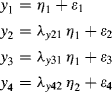
The measurement equation ![]() can be expressed as:
can be expressed as:
where the ![]() matrix decides which observed endogenous y indicators are loaded onto which endogenous
matrix decides which observed endogenous y indicators are loaded onto which endogenous ![]() latent variables. The fixed value of 0 indicates the corresponding indicators are not loaded onto the corresponding latent variables, while the fixed value of 1 is used for the purpose of model identification and defining the scale of the latent variable. We will discuss this issue in detail later in Chapter 2.
latent variables. The fixed value of 0 indicates the corresponding indicators are not loaded onto the corresponding latent variables, while the fixed value of 1 is used for the purpose of model identification and defining the scale of the latent variable. We will discuss this issue in detail later in Chapter 2.
From Equation (1.4) we have the following four measurement structural equations:
As the second endogenous latent variable ![]() has only one indicator (i.e., y4), thus
has only one indicator (i.e., y4), thus ![]() should be set to 1.0, thus
should be set to 1.0, thus ![]() . As it is hard to estimate the measurement error in such an equation in SEM, the equation is usually set to
. As it is hard to estimate the measurement error in such an equation in SEM, the equation is usually set to ![]() , assuming that the latent variable
, assuming that the latent variable ![]() is perfectly measuring the single indicator y4. However, if the reliability of y4 is known, based on empirical finding or estimated from item reliability study, the variance of
is perfectly measuring the single indicator y4. However, if the reliability of y4 is known, based on empirical finding or estimated from item reliability study, the variance of ![]() in the equation
in the equation ![]() can be estimated and specified in the model to take into consideration the effect of measurement errors in y4. We will demonstrate how to do this in Chapter 3.
can be estimated and specified in the model to take into consideration the effect of measurement errors in y4. We will demonstrate how to do this in Chapter 3.
Another measurement equation ![]() can be expressed as:
can be expressed as:
Thus,
(1.7) 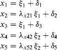
Among the seven random variable vectors (![]() ,
, ![]() ,
, ![]() , x, y,
, x, y, ![]() , and
, and ![]() ), x, y,
), x, y, ![]() , and
, and ![]() are usually used together with the eight-parameter matrices to define a SEM model; the others are error terms or model residuals. It is assumed that E (ζ) = 0, E (ε) = 0, and E (δ) = 0, Cov (ζ,ξ) = 0, Cov (ε,η) = 0, and Cov (δ,ξ) = 0. In addition, multivariate normality is assumed for the observed and latent variables.
are usually used together with the eight-parameter matrices to define a SEM model; the others are error terms or model residuals. It is assumed that E (ζ) = 0, E (ε) = 0, and E (δ) = 0, Cov (ζ,ξ) = 0, Cov (ε,η) = 0, and Cov (δ,ξ) = 0. In addition, multivariate normality is assumed for the observed and latent variables.