7 Visual Cryptography and Random Grids

A random grid was defined by Kafri and Keren in 1987 [7] as a transparency comprising a two-dimensional array of pixels. Each pixel is either fully transparent or simply opaque and the choice between the alternatives is made by a coin-flip procedure. Thus, there is no correlation between the values of different pixels in the array.

We could encrypt binary pictures or shapes into two random grids such that only the areas containing information in the two grids are intercorrelated, while the others are purely random. When the two grids are superimposed together, the correlated areas will be resolved from the random background due to the difference in light transmission so that the secret picture or shape can be seen visually. Just like conventional schemes in visual cryptography, the decoding process is done by the human visual system where no computation is needed; however, no extra pixel expansion is required using random grids.

Observing the interesting features of random grids in image encryption, which were discussed right before Naor and Shamir's visual cryptographic scheme (VCS) [9], Shyu [12, 13] generalized the random grids-based approaches into visual cryptograms of random grids (VCRG) for achieving visual secret sharing recently. The most appealing benifits using random grids lie in that the pixel expansion needed is merely one and no basis matrix is needed. With the same contrast in the reconstructed results, the optimal pixel expnasion in (n, n)-VCS is 2ⁿ⁻¹; while that in (n, n)-VCRG is still 1.

We study the random grids-based schemes, analyze the performances, and demonstrate their feasibilities in this chapter. The rest of the chapter is organized as follows. The fundamental characteristics of random grids are discussed in Section 7.2. Section 7.3 discusses how to apply visual cryptograms of random grids in visual cryptography where the formal definition of VCRG is given, and the designs, analyses, and implementations of (2, 2)-VCRGs and (n, n)-VCRGs for binary, gray-level and color images are examined. Section 7.4 exhibits some concluding remarks.

7.2 Random Grids

7.2.1 Random Pixel, Random Grid, and Average Light Transmission

We refer to a binary pixel r as a random pixel if the choice for r to be transparent or opaque in R is totally random; or equivalently, the probability for r to be transparent is equal to that for r to be opaque,

P r o b (r = 0) = P r o b (r = 1) = \frac{1}{2}, (7.1)

$P r o b (r = 0) = P r o b (r = 1) = \frac{1}{2}, (7.1)$

where 0 (1) denotes a transparent (opaque) pixel. Since a transparent pixel lets through the light while an opaque one stops it, the average light transmission of random pixel r is $\frac{1}{2}$ $\frac{1}{2}$ , denoted as

t (r) = \frac{1}{2} . (7.2)

$t (r) = \frac{1}{2} . (7.2)$

Definition 1 R is a binary random grid if each pixel r in R is a binary random pixel.

Regarding a random grid R, the number of transparent pixels is probabilistically the same as that of opaque ones so that the average light transmission of R is also $\frac{1}{2}$ $\frac{1}{2}$ , denoted as

J (R) = \frac{1}{2} . (7.3)

$J (R) = \frac{1}{2} . (7.3)$

7.2.2 Superimposition of Random Grids

Let ⊗ denote the generalized ”or” operation, which describes the relation of the superimposition of two random pixels or grids pixel by pixel. It is obvious that r ⊗ r (R ⊗ R) is entirely the same as r (R), that is

t (r \otimes r) = \frac{1}{2} or J (R \otimes R) = \frac{1}{2} (7.4)

$t (r \otimes r) = \frac{1}{2} or J (R \otimes R) = \frac{1}{2} (7.4)$

for each pixel r in R.

Let R₁ and R₂ be two independent random grids with the same size. When R₁ and R₂ are superimposed pixel by pixel, each pixel (either transparent or opaque) in R₁ has an equal possibility to be stacked by a transparent pixel or an opaque pixel in R₂.We call r₁ = R₁[i,j] the corresponding pixel of r₂ = R₂[i′, j′] if and only if i = i′ and j = j′ (the positions of r₁ at R₁ and r₂ at R₂ are the same). It is easy to see that the order of the two random grids does not affect the superimposed result, i.e.,

R_{1} \otimes R_{2} = R_{2} \otimes R_{1} . (7.5)

$R_{1} \otimes R_{2} = R_{2} \otimes R_{1} . (7.5)$

Indeed, ⊗ is a commutative operation.

Table 7.1 Results of the superimposition of two random pixels.

r₁	r₂	r₁ ⊗ r₂
0	0	0
0	1	1
1	0	1
1	1	1

Table 7.1 shows the superimposed results of the corresponding random pixels r₁ and r₂. There is only one outcome among the four possible combinations of r₁ ⊗ r₂ showing transparency. Since the four possible combinations occur with an equal probability, the probability for r₁ ⊗ r₂ to be transparent is $\frac{1}{4}$ $\frac{1}{4}$ . That is, the average light transmission of the superimposition of R₁ and R₂ (r₁ and r₂) is $\frac{1}{4}$ $\frac{1}{4}$ .

We summarize the aforementioned properties in Lemma 1.

Lemma 1 If R₁ and R₂ are two independent random grids with J(R₁) = J (R₂) = 1/2,

J(R₁ ⊗ R₂) = J(R₂ ⊗ R₁) = 1/4;
J(R₁ ⊗ R₁) = 1/2.

We define $\bar{R}$ $\bar{R}$ to be the inverse random grid of R if and only if

r^{'} = \bar{r}

$r^{'} = \bar{r}$

for each r′ in $\bar{R}$ $\bar{R}$ where r is the corresponding pixel of r′ in R and r̄ denotes the inverse of r. It is easy to see that r ⊗ r̄ = 1 and $R \otimes \bar{R} = 1$ $R \otimes \bar{R} = 1$ (1 denotes a grid in which all pixels are opaque), that is

t (r \otimes \bar{r}) = 0 and J (R \otimes \bar{R}) = 0 (7.6)

$t (r \otimes \bar{r}) = 0 and J (R \otimes \bar{R}) = 0 (7.6)$

For each pixel r′ in $\bar{R}$ $\bar{R}$ , since $P r o b (r^{'} = 0) = P r o b (\bar{r} = 0) = P r o b (r = 1) = \frac{1}{2}$ $P r o b (r^{'} = 0) = P r o b (\bar{r} = 0) = P r o b (r = 1) = \frac{1}{2}$ , we obtain

t (\bar{r}) = \frac{1}{2} and J (\bar{R}) = \frac{1}{2} (7.7)

$t (\bar{r}) = \frac{1}{2} and J (\bar{R}) = \frac{1}{2} (7.7)$

In general, the relationship of the average light transmissions of R ∈ R is given in Lemma 2.

Lemma 2 If R is a random grid with J(R) = λ, $J (\bar{R}) = 1 - λ$ $J (\bar{R}) = 1 - λ$ .

Proof From J(R) = λ, we know that for any pixel r ∈ R Prob (r = 0) = λ and Prob(r = 1) = 1 − λ. Let $r^{'} \in \bar{R}$ $r^{'} \in \bar{R}$ be the corresponding pixel of r. Thus, Prob(r′ = 1)= Prob(r = 1) = 1 − λ and Prob(r′ = 1) = Prob(r = 1) = λ. We have $J (\bar{R}) = 1 - λ$ $J (\bar{R}) = 1 - λ$ . ■

Consider two independent random grids X and Y. There is another important property called the principle of combination : if we cut a section, say A, from X and replace it with section B (with the same size as A) from Y, the result, denoted as Z = (X A) ∩ B, is another random grid, i.e.,

J (Z) = J (X) = J (Y) = \frac{1}{2} (7.8)

$J (Z) = J (X) = J (Y) = \frac{1}{2} (7.8)$

We shall expose how to use the aforemnetioned characteristics of random grids to accomplish visual secret sharing in the next section.

7.3 Visual Cryptograms of Random Grids

First of all, we give a formal definition to VCRG for binary images in Section 7.3.1. Section 7.3.2 presents three algorithms for producing (2, 2)-VCRGs for binary images. The implementation results of these algorithms are reported in Section 7.3.3. Section 7.3.4 evaluates the performances of these algorithms in terms of light contrast. Then, algorithms for producing (n, n)-VCRGs for binary images are discussed in Section 7.3.5. Further, those for gray-level and color images are examined in Section 7.3.6. Section 7.3.7 reports the experimental results of (n, n)-VCRGs. The correctness of these algorithms would be proved and the corresponding light contrasts would be analyzed accordingly.

7.3.1 Definition of VCRG

Consider a set of n random grids E = {R₁, R₂,…, R_n}, which are encrypted to share a a secret image B such that R₁ ⊗ R₂ ⊗… ⊗ R_n reveals B to our eyes while any group of less than n grids obtains no information about B. We call E a set of visual cryptograms of random grids with respect to B.

Let B(0) (B(1)) denote the area of white (black) pixels in B and S^E [B(0)] (S[B(1)]) denotes the area of pixels in S^E corresponding to B(0) (B(1)) where S^E = R₁ ⊗ R₂ ⊗⋯⊗R_n. Formally, a set of (n, n) visual cryptograms of random grids for a binary image is now defined as follows.

Definition 2 Given a binary image B, n random grids {R₁, R₂,…, R_n} comprise a set of visual cryptograms, referred to as (n, n)-VCRG of B if the following conditions hold:

R_i is a random grid with J(R_i) = 1/2 for 1 ⩽ i ⩽ n;
J(S^D[B(0)]) = J(S^D[B(1)]) where $S^{D} = R_{i_{1}} \otimes R_{i_{2}} \otimes \dots \otimes R_{i_{d}}$ $S^{D} = R_{i_{1}} \otimes R_{i_{2}} \otimes \dots \otimes R_{i_{d}}$ which is the superimposed result of some set $D = {R_{i_{1}}, R_{i_{2}}, \dots, R_{i_{d}}}$ $D = {R_{i_{1}}, R_{i_{2}}, \dots, R_{i_{d}}}$ of d distinct random grids in E, i.e., D ⊂ E, 2 ⩽ d ⩽ n − 1 and 1 ⩽ i₁ < i₂ < ⋯< i_d ⩽ n; and
J(S^E[B(0)]) > J(S^E[B(1)]) where S^E = R₁ ⊗ R₂ ⊗ … ⊗ R_n and E = {R₁, R₂, … , R_n}.

Both Conditions 1 and 2 are ”security” conditions which ensure that each individual grid and the superimposed result of any group of less than n random grids are merely random grids so that no information of B can be obtained. Condition 3 is the ”contrast” condition, which claims that once the light transmission of S^E[B(0)] is larger than that of S^E [B(1)], our visual perception is able to distinguish B(0) from B(1) by observing S^E due to the difference of their light transmissions in S^E.

Note that this definition is different from that in Naor and Shamir’s model. Suppose that C₁ and C₂ are the two encoded shares produced by some (2, 2)-VCS using basis matrices M⁰ and M¹ with respect to binary image B. Then the security condition in (2, 2)-VCS is w(M^b[1]) = (M^b[2]) for b ∈ {0, 1} where M^b[i] is the ith row of M^b for i ∈ {1, 2}, while the contrast condition becomes w(M¹[1]or M¹[2]) − (M⁰[1] or M⁰[2]) > 0. Let c₁ in C₁ and c₂ in C₂ be the corresponding pixels of b in B. Let d = c₁ ⊗ c₂ where d is in D = C₁ ⊗ C₂. Let b(0) (b(1)) denote the pixel of b = 0(1) and d[b(0)] (d[b(1)]) denote such d corresponding to b(0) (b(1)). Since each b = 0 (1) is encoded according to M⁰ (M¹ ), the contrast condition in (2, 2)-VCS assures w(d[b(1)])−w(d[b(0)]) > 1 so that d(1) can be identified from d(0) for all d(0)’s and d(1)’s in D. However, VCRG only demands J(S[B(0)]) −J(S[B(1)]) > 0, or equivalently, t(s[b(0)]) − t(s[b(1)]) > 0.

7.3.2 (2, 2)-VCRG Algorithms for Binary Images

Let random_pixel(0, 1) be a function that returns a binary value 0 or 1 to represent a transparent or opaque pixel, respectively, by a coin-flip procedure and $R_{1} [i, j]$ $R_{1} [i, j]$ denote the complement of R₁[i, j]. Each of the following three algorithms successfully encodes a secret binary image B into two random grids R₁ and R₂ which constitute a set of (2, 2)-VCRG.

Algorithms 1–3. Sharing a binary image by two random grids

Input: A w × h binary image B where B[i, j] ∈ {0, 1} (white or black), 1⩽i⩽w and 1⩽j⩽h

Output: Two shares of random grids R₁ and R₂ which reveal B when superimposed where R_k[i, j] ∈ {0, 1} (transparent or opaque), 1⩽i⩽w, 1⩽j ⩽h and k ∈ {1, 2}

Encryption(B)

Algorithm 1.

1. Generate R₁ as a random grid, J(R₁) = 1/2

// for (each pixel R₁[i, j], 1⩽i⩽w, and 1⩽j⩽h) do

// R₁[i,j] = random_pixel (0, 1)

2. for (each pixel B[i, j], 1⩽i ⩽w and 1⩽j ⩽h) do

2.1 { if (B[i, j]=0) then R₂[i,j] = R₁[i,j]

else $R_{2} [i, j] = \bar{R_{1} [i, j]}$ $R_{2} [i, j] = \bar{R_{1} [i, j]}$

3. output(R₁, R₂)

Algorithm 2.

1. Generate R₁ as a random grid, J(R₁) = 1/2

2. for (each pixel B[i, j], 1⩽i⩽w and 1⩽j⩽h) do

2.1 { if (B|i, j|=0) then R₂|i, j| = R₂|i, j|

else R₂[i, j] = random_pixel(0, 1)

}

3. output(R₁, R₂)

Algorithm 3.

1. Generate R₁ as a random grid, J(R₁) = 1/2

2. for (each pixel B[i, j], 1⩽i⩽w and 1⩽j⩽h) do

2.1 { if (B[i, j] = 0) then R₂[i, j] = random_pixel(0, 1)

else $R_{2} [i, j] = \bar{R_{1} [i, j]}$ $R_{2} [i, j] = \bar{R_{1} [i, j]}$

}

3. output(R₁, R₂)

The three algorithms are capsulated into a generic procedure named Encryption so that when Encryption(B) is called, each of Algorithms 1, 2, or 3 can be applied onto B. Also note that in this paper, 0 (1) denotes a white (black) pixel in the secret binary image or a transparent (opaque) pixel in the encrypted share interchangeably.

Table 7.2 summarizes the encoding process of pixel b in secret image B into r₁ and r₂ by Algorithms 1, 2, and 3 respectively, the result of r₁ ⊗ r₂ and its average light transmission.

Let B(0) (B(1)) denote the area of all of the transparent (opaque) pixels in B, that is, pixel b is in B(0) (B(1)) if and only if b = 0 (b = 1) where B = B(0) ∪ B(1) and B(0) ∩ B(1) = Ø. We denote the area of pixels in random grid R corresponding to B(0) (B(1)) by R[B(0)] (R[B(1)]), that is, pixel r is in R[B(0)] (R[B(1)]) if and only if r’s corresponding pixel b is in B(0) (B(1)). Surely, R = R[B(0)] ∪ R[B(1)] and R[B(0)] ∩ R[B(1)] = Ø.

Based upon the above notations, we have the following theorem.

Theorem 1 Given a binary image B, {R₁, R₂} produced by Algorithms 1−3, respectively, is a set of (2, 2)-VCRG of B.

Images

Table 7.2 Encoding b into r₁ and r₂ and results of s = r₁ ⊗ r₂ by Algorithms 1, 2, and 3.

Proof To prove that R₁ and R₂ constitute a set of (2, 2)-VCRG, we should validate whether the following two conditions (setting n = 2 in Definition 2) hold:

J(R₁) = J(R₂) $\frac{1}{2}$ $\frac{1}{2}$ ; and
J(S[B(0)]) > J(S[B(1)]) where S = R₁ ⊗ R₂.

Let us examine Algorithm 1 first. Let R₁ [B(b)] denote the area of pixels in R₁ that corresponds to B(b) for b = 0 or 1. Note that R₁ = R₁[B(0)] ∪ R₁[B(1)] where R₁[B(0)] ∩ R₁[B(1)] = Ø. Since Step 1 in Algorithm 1 composes R₁ as a random grid with J(R₁) =1/2, we have R₁(R₁) = R(R₁[B(0)]) = J(R₁[B(1)]) = 1/2. When B[i, j] = 0, we have R₂[i, j] = R₁[i, j]. That means J(R₂ |B(0)|) = J(R₁[B(0)]) = 1/2. Moreover, when B[i, j] = 1, $R_{2} [i, j] = \bar{R_{1} [i, j]}$ $R_{2} [i, j] = \bar{R_{1} [i, j]}$ . By Lemma 2, we have $J (R_{2} [B (1)]) = J ({\bar{R}}_{1} [B (1)]) = 1 - J (R_{1} [B (1)]) = 1 - 1 / 2 = 1 / 2$ $J (R_{2} [B (1)]) = J ({\bar{R}}_{1} [B (1)]) = 1 - J (R_{1} [B (1)]) = 1 - 1 / 2 = 1 / 2$ . Due to the facts that R₂ = R₂[B(0)] ∪ R₂[B(1)] and J(R₂[B(0)]) = J(R₂[B(1)]) = 1/2, we have J(R₂) = 1/2 by the principle of combination. Therefore both of R₁ and R₂ are merely random grids and none of them individually leaks any information about B. Jhe security condition of Definition 2 is met.

Consider B(0) (the ares of transparent pixels in B). Since R₂[i, j] = R₁[i, j] for each B[i, j] = 0 (or B[i, j] ∈ B(0)), thus S[B(0)] = R₁[B(0)] ⊗ R₂[B(0)] = R₁[B(0)]. Jhus J(S[B(0)]) = 1/2. Regarding B(1), $R_{2} [i, j] = \bar{R_{1} [i, j]}$ $R_{2} [i, j] = \bar{R_{1} [i, j]}$ for each B[i, j] = 1 (or B[i, j] ∈ B(1)). We have S|B(1)| = R₁[B(1)] ⊗ R₂[B(1)] = 1 (an area with all opaque pixels), i.e., J(S[B(1)]) = 0. Jhus J(S[B(0)]) > J(S[B(1)]). Jhe light contrast condition of Definition 2 is satisfied. Jherefore, {R₁, R₂} produced by Algorithm 1 is a set of (2, 2)-VCRG of B and (J(S[B(0)]), J(S[B(1)])) = (1/2, 0).

For Algorithm 2, we have J(R₂[B(0)]) = J(R₁[B(0)]) = 1/2 and R₂[B(1)] is purely a random grid with J(R₂[B(1)]) = 1/2. Jhus, R₂ is a random grid with J(R₂) = 1/2. Since R₂[B(0)] = R₁[B(0)], J(S[B(0)]) = J(R₁|B(0)| ⊗ R₂|B(0)| = J((R₁|B(0)|) = 1/2; while R₁|B(1)| and R₂|B(1)| are two independent random grids so that J(S[B(1)]) = J(R₁[B(1)] ⊗ < R₂[B(1)]) = J(R₁[B(1)]) × J(R₂[B(1)]) = 1/4 (by Lemma 1(1)). We obtain J(S[B(0)]) > J(S[B(1)]).

For Algorithm 3, J(R₂[B(0)]) = 1/2 because R₂[B(0)] is a purely random grid and $J (R_{2} [B (1)]) = J (\bar{R_{2}} [B (1)]) = 1 - J ((R_{1} [B (1)]) = 1 / 2$ $J (R_{2} [B (1)]) = J (\bar{R_{2}} [B (1)]) = 1 - J ((R_{1} [B (1)]) = 1 / 2$ . We have J(R₂) = 1/2. Further, due to the fact that R₁ [B(0)] and R₂[B(0)] are independent, J(S[B(0)]) = J(R1[B(0)] ⊗ J R₂[B(0)]) = J(R₁[B(0)]) × J(R₂[B(0)]) = 1/4; on the other hand, since $R_{2} [B (1)] = \bar{R_{1}} [B (1)]$ $R_{2} [B (1)] = \bar{R_{1}} [B (1)]$ , S[B(1)] = R₁ [B(1)] ⊗ (R₂[B(1)] = 1, i.e. J(S[B(1)] = 0. We have J(S[B(0)]) > J(S[B(1)]).

Based upon the above statements, we realize that both security and contrast conditions in Definition 2 hold for all of the three algorithms. We conclude that no information of B can be obtained from random grids R₁ or R₂ individually, while S reveals B in our visual system for all of the three algorithms. Jheorem 1 is proved.

The following corollary is an immediate consequence from the statements in the proof of Jheorem 1.

Corollary 1 (J(S[B(0)]), J(S[B(1)])) = (1/2, 0), (1/2, 1/4) or (1/4, 0) for Algorithms 1–3, respectively where S = R₁ ⊗ R₂ and {R₁, R₂} is a set of (2, 2)-VCRG produced by Algorithms 1–3 with respect to secret image B.

7.3.3 Experiments for (2, 2)-VCRG

Figure 7.1 illustrates the results of the implementation of the above three algorithms. Figure 7.1(a) is secret binary image B, Figures 7.1(b) and (c) present the two random grids produced by Algorithm 1 and Figure 7.1(d) is the superimposed result of these two shares ((b) and (c)). Figures 7.1(e)–g) illustrate the corresponding results by Algorithm 2, while Figures 7.1(h)–(j) are the corresponding results by Algorithm 3. It can be easily seen from Figure 7.1 that the encrypted shares (see Figure 7.1(b), (c), (e), (f), (h), and (i)) are merely random pictures and no information about B can be obtained. Only when the two shares are superimposed (see Figures (d), (g), and (j)), can we see B by our visual system. It is worthy of notifying that there is no extra pixel expansion in Figures 7.1(b)–(j).

Figure 7.2 shows the reconstructed results by using Naor and Shamir’s approach for encrypting B in Figure 7.1(a). The pixel expansion of Figure 7.2(a) is 2, while that of Figure 7.2(b) is 4 ( by applying $S^{0} = [\begin{array}{l} 0 & 1 & 0 & 1 \\ 0 & 1 & 0 & 1 \end{array}]$ $S^{0} = [\begin{array}{l} 0 & 1 & 0 & 1 \\ 0 & 1 & 0 & 1 \end{array}]$ and $S^{1} = [\begin{array}{l} 0 & 1 & 0 & 1 \\ 1 & 0 & 1 & 0 \end{array}])$ $S^{1} = [\begin{array}{l} 0 & 1 & 0 & 1 \\ 1 & 0 & 1 & 0 \end{array}])$ . Jhe former does not retain the aspect ratio with respect to B, while the latter does. Both sizes of the results in Figure 7.2 are larger than that of B.

7.3.4 Definition of Light Contrast and Performance Evaluation

To evaluate the relative difference of the light transmissions between the transparent and opaque pixels in reconstructed image S by these random grid-based algorithms, we define the light contrast of S with respect to B as follows.

Definition 3 Jhe light contrast of a set E of VCRG produced by an encryption algorithm for a binary image B is defined as

c (ℰ) = \frac{J (S [B (0)]) - J (S [B (1)])}{1 + J (S [B (1)])}

$c (ℰ) = \frac{J (S [B (0)]) - J (S [B (1)])}{1 + J (S [B (1)])}$

where S is the superimposed result of all visual cryptograms in E.

Let E₁, E₂, and E₃ denote the three sets of (2, 2)-VCRG produced by Algorithms 1–3, respectively. By Definition 3, the light contrasts of E₁, E₂, and E₃ are c(E₁) = 1/2 (= (1/2 − 0)/(1 + 0)), c(E₂) = 1/5 (= (1/2 − 1/4)/(1 + 1/4)), and c(E₃) = 1/4 (= (−1/4 − 0)/(1 + 0)). Jhat is, Algorithm 1 achieves the highest light contrast among the three. Jhis outcome can also be observed by comparing the reconstructed images in Figures 7.1(d), (g), and (j) in which (d) is more recognizable than (g) and (j). Note that 1 + J(S[B(1)]) is introduced as the denominator of c(E) in favor of a less J(S[B(1)]) (than a larger one) when two schemes have a same numerator (i.e., J(S[B(0)]) − T(S[B(1)])). For instance, both of E₂ and E₃ have the same result of J(S[B(0)]) − T(S[B(1)])), yet their J(S[B(1)])’s are 1/4 and 0, respectively. Jhus, c(E₃) > c(E₂) according to Definition 3. As we can see, the reconstructed image by E₃ (Figure 7.1(j)) is indeed more recognizable than that by E₂ (Figure 7.1(g)) by our visual system. In general, we prefer a set of VCRG with a larger light contrast that helps our visual perception to recognize the result. Thus, Algorithm 1 is more preferable than the other two.

Images

FIGURE 195.7
Implementation results of Algorithms 1, 2, and 3 for encrypting binary image B: (a) B; (b), (c), and (d) two encrypted shares and reconstructed image by Algorithm 1; (e), (f), and (g) two encrypted shares and reconstructed image by Algorithm 2; (h), (i), and (j) two encrypted shares and reconstructed image by Algorithm 3.

Images

FIGURE 196.7
Reconstructed results by Naor and Shamir’s approach for binary image B in Figure 7.1(a): (a) m = 2, (b) m = 4.

We summarize the reconstructed light contrasts by these three algorithms in Jable 7.3.

Table 7.3 Light contrasts by Algorithms 1–3 in producing VCRG-2.

E	J (S[B(0)])	J (S[B(1)])	c(E)
Algorithm 1	$\frac{1}{2}$ $\frac{1}{2}$	0	$\frac{1}{2}$ $\frac{1}{2}$
Algorithm 2	$\frac{1}{2}$ $\frac{1}{2}$	$\frac{1}{4}$ $\frac{1}{4}$	$\frac{1}{5}$ $\frac{1}{5}$
Algorithm 3	$\frac{1}{4}$ $\frac{1}{4}$	0	$\frac{1}{4}$ $\frac{1}{4}$

It is noticed that various definitions of contrast in [9, 14, 1] all depend on pixel expansion so that they are not suitable any more to measure the effectiveness of our schemes. On the contrary, since we consider the light transmissions through different areas of the transparency, the measurement of light contrast is more generalized and can be applied to all kinds of schemes.

We discuss how to generate (n, n)-VCRG in the next subsection.

7.3.5 Algorithms of (n, n)-VCRG for Binary Images

Consider an h × w binary image B and n random grids R₁, R₁, …, R_n with the same dimension. We call r₁, r₂, …, r_n the corresponding pixels of b ∈ B if all r_k’s in R_k’s for 1 ⩽ k ⩽ n have the same coordinates as b (if b = B[i, j], then r_k = R_k [i, j] where 1 ⩽ i ⩽ h and 1 ⩽ j ⩽ w).

By extending the idea of Algorithm 2 directly, we may obtain a set of two out of n visual cryptograms of random grids where any pair of two out of the n shares can reveal the secret when superimposed. Given a binary image B, we first find a random grid R₁ with J(R₁) = 1/2. Jhen, we define R_k for 2 ⩽ k ⩽ n as follows:

r^{k} = {\begin{array}{l} r_{1} & if b = 0; \\ r a n d o m_p i x e l () & otherwise, \end{array} (7.9)

$r^{k} = {\begin{array}{l} r_{1} & if b = 0; \\ r a n d o m_p i x e l () & otherwise, \end{array} (7.9)$

for each pixel r_k ∈ R_k where r₁, r₂, …, r_n are corresponding pixels of b ∈ B. It is easy to see that all R_k’s are random grids and when b = 0, t(r_j ⊗ r_j) = t/(r₁ ⊗ r₁) = t(r₁) = 1/2; while b =1, t(r_i ⊗ r_j) = 1/4 by Lemma 1 for each pair of i and j where 1 ⩽ i ≠ j ⩽ n. Jhat is, J(R_i[B(0)] ⊗ R_j[B(0)]) = 1/2 > 1/4= J(R_i[B(1)] ⊗ R_j [B(1)]). As a result, {R₁, R₂, …, R_n} produced in this way is a set of two out of n visual cryptograms of random grids. Yet, it is not a set of (n, n)-VCRG, since Condition 2 in Definition 2 fails.

Let us extract some informative features from the idea in Algorithm 1. Let B = {0, 1} be a binary set. We introduce a function f : B × B → B defined as follows to transcribe the basic idea in Algorithm 1:

f (x, s) = {\begin{array}{l} s & if x = 0; \\ \bar{s} & otherwise, \end{array} (7.10)

$f (x, s) = {\begin{array}{l} s & if x = 0; \\ \bar{s} & otherwise, \end{array} (7.10)$

for x, s, $\bar{S}$ $\bar{S}$ ∈ B where $\bar{S}$ $\bar{S}$ is the inverse value of s. We may say that function f(x, s) preserves the value of s if x = 0, and reverses it otherwise (x = 1). In the subject of sequential circuits, the behavior of f(x, s) is equivalent to that of a T flip-flop where s, x and f(x, s) are the current state, toggle input, and next state, respectively. In the area of logical operations, f(x, s) can be implemented by using the Exclusive-OR operation (⊕), that is, f(x, s) = x ⊕ s.

Let B be a binary image and R₁ be a random grid with J(R₁) = 1/2. By introducing function f, the essential idea of Algorithm 1 for generating each pixel r₂ ∈ R₂ corresponding to r₁ ∈ R₁ and b ∈ B can be formulated as

r_{2} = f (b, r_{1}) . (7.11)

$r_{2} = f (b, r_{1}) . (7.11)$

Note that when b = 0, r₂ = r₁; while b = 1, $r_{2} = \bar{r_{1}}$ $r_{2} = \bar{r_{1}}$ . This is exactly the same as the manipulation of Step 2 in Algorithm 1.

This critical observation is emphasized as a corollary as follows.

Corollary 2 If R₁ is a random grid with J(R₁) = 1/2 and the corresponding pixel r₂ ∈ R₂ of r_i ∈ R₁ is obtained by r₂ = f(b, r₁) for each r₁ ∈ R₁ with any b ∈ B, then R₂ is a random grid with J(R₂) = 1/2.

By using function f, our first construction of a set of (n, n)-VCRG (E = {R₁, R₂, ..., R_n}) with respect to B is now introduced as follows. We first generate n − 1 random grids R₁, R₂, ..., R_n−1 independently with J(R_k) = 1 / 2 for 1 ⩽ k ⩽ n − 1. Jhat is, for every pixel b ∈ B its n − 1 corresponding pixels r₁, r₂, …,r_{n − 1} are totally random where r_k ∈ R_k for 1 ⩽ k ⩽ n − 1. Based upon r₁, r₂, …,r_k, we compute a_k for 1 ⩽ k ⩽ n − 1 by using the recursive formula:

a_{k} = {\begin{array}{l} r_{1} & if k = 1; \\ f (r_{k}, a_{k - 1}) & otherwise . \end{array} (7.12)

$a_{k} = {\begin{array}{l} r_{1} & if k = 1; \\ f (r_{k}, a_{k - 1}) & otherwise . \end{array} (7.12)$

Then, we find r_n according to b and α_n−1 by

r_{n} = f (b, a_{n - 1}) . (7.13)

$r_{n} = f (b, a_{n - 1}) . (7.13)$

It is noticed that formula (7.11) is a special case of formula (7.13) by setting n = 2. After all r_n’s ∈ R_n corresponding to all b’s ∈ B are computed, we obtain R_n. Then, E = {R₁, R₂,…, R_n} is reported as a set of (n, n)-VCRG of B. The whole idea is formally illustrated in Algorithm 4.

Algorithm 4. Encrypting a secret image into a set of (n, n)-VCRG

Input: an h × w binary image B and an integer n

Output: E = {R₁, R₂,…, R_n} constituting (n, n)-VCRG of B

1. for (1 ⩽ k ⩽ n − 1) do

{ generate R_k as a random grid, J(R_k) = 1/2

2. for (each pixel B[i, j], 1 ⩽ i ⩽ h and 1 ⩽ j ⩽ w) do

2.1 { a₁ = R₁[i,j]

2.2 for (2 ⩽ k ⩽ n − 1) do

{a_k = f(R_k [i, j], a_k−1) //f(x, s) is defined in formula (7.10)

2.3 R_n[i,j]= f(B[i,j],a_n−1)

3. output(R₁, R₂,…, R_n)

Before we prove that E = {R₁,R₂,…,R_n} generated by Algorithm 4 with respect to B is indeed a set of (n, n)-VCRG of B, we explore more useful features among multiple random grids in the following.

It is easy to see that two independent random grids produce another random grid as they are superimposed even when their light transmission is not 1/2. We formalize this in Lemma 3, which is a generalized version of Lemma 1.

Lemma 3 Given two independent random grids R₁ and R₂ with J(R₁) = λ₁ and J(R₂) = λ₂, R₁ ⊗ R₂ is a random grid with J(R₁ ⊗ R₂) = λ₁λ₂.

Proof For any pixel r₁ ∈ R₁ and its corresponding pixel r₂ ∈ R₂, we have Pwb(r₁ = 0) = λ₁ and Pwb(r₂ =0) = λ₂. r₁ ⊗ r₂ is transparent if and only if both of r₁ and r₂ are transparent, that is, Pwb(r₁ ⊗ r₂ = 0) = Pwb(r₁ = 0) × Pwb(r₂ = 0) = λ₁λ₂. Therefore, J(R₁ ⊗ R₂) = J(R_i) × J(R₂) = λ₁λ₂.

The theme of Lemma 3 can be extended for more than two random grids.

Lemma 4 If U = {R₁, R₂, …, R_u} is a set of u ≥ 2 independent random grids with J(R_i) = λ for 1 ≤ i ≤ u, then S^U is a random grid with J(S^U) = λ^u where S^U = R₁ ⊗ R₂ ⊗ ⋯ ⊗ R_u.

Proof We prove by mathematical induction. Consider the case of V = {R₁, R₂}. The statement (i.e., J(S^V) = λ²) is true by Lemma 3. Assume that the statement holds for the case of V = {R₁, R₂,…, R_u−1}, that is, S^V is a random grid with J(S^V) = λ^u−1 where S^V = R₁ ⊗ R₂ ⊗ ⋯ ⊗ R_u−1. Then, we further consider U = {R₁, R₂,…, R_u} = V ∪ {R_u}. S^U is simply the superimposed result of S^V and R_u, i.e., S^U = S^V ⊗ R_u. By Lemma 3, we have J(S^U) = J(S^V ⊗ R_u) = J(S^V) × J(R_u) = (λ^u−1) × λ = λ^u.

Since the superimposition operation ⊗ is commutative, it is not hard to obtain that the results of different superimposing orders of R₁, R₂,…, R_u are all the same (i.e., S^U). As a matter of fact, the superimposed result of any subset of U is also a random grid as indicated in Lemma 5.

Lemma 5 Let U = {R₁, R₂, …, R_u} be a set up u ≥ 2 independent random grids and $V = {R_{i_{1},} R_{i_{2}, \dots,} R_{i_{v},}} \subset U$ $V = {R_{i_{1},} R_{i_{2}, \dots,} R_{i_{v},}} \subset U$ where 1 ≤ i₁ < i₂ < ⋯ < i_v ≤ u and J(R_i) = λ for 1 ≤ i ≤ u. S^V is a random grid with J(S^V) = λ^v where $S^{V} = R_{i_{1}} \otimes R_{i_{2}} \otimes \dots \otimes R_{i_{v}}$ $S^{V} = R_{i_{1}} \otimes R_{i_{2}} \otimes \dots \otimes R_{i_{v}}$ .

The proof of Lemma 4 can be easily applied to prove Lemma 5. Consider a set of u independent random grids U = {R₁, R₂,…, R_u} where J(R_k) = 1/2 for 1 ≤ k ≤ u. We may generate a set of u binary images A = {A₁, A₂,…, A_u} with respect to U in such a way that each pixel a_k ∈ A_k is defined by formula (7.12), that is,

a_{k} = {\begin{array}{l} r_{1} & if k = 1; \\ f (r_{k}, a_{k - 1}) & otherwise, \end{array}

$a_{k} = {\begin{array}{l} r_{1} & if k = 1; \\ f (r_{k}, a_{k - 1}) & otherwise, \end{array}$

where a_k ∈ A_k and r_k ∈ R_k are corresponding pixels for 1 ≤ k ≤ u. Lemma 6 claims that all of A₁, A₂,…, A_u are random grids with J(A_k) = 1/2 for 1 ≤ k ≤ u.

Lemma 6 For A = {A₁, A₂,…, A_u} generated by formula (7.12) with respect to U = {R₁, R₂,…, R_u} where J(R_k) = 1/2, A_k is a random grid with J(A_k) = 1/2 for 1 ≤ k ≤ u.

Proof We prove by mathematical induction. For the case of |A| = 1 (i.e., u = 1), since a₁ ∈ A₁ is equal to r₁ ∈ R₁ by formula (7.12), A₁ is exactly the same as R₁. Thus, A₁ is a random grid with J(A₁) = J(R₁) = 1/2. Assume that the statement holds for the case of |A| = u − 1, that is, A₁, A₂,…, A_u−1 are random grids with J(A_k) = 1/2 for 1 ≤ k ≤ u − 1. Due to the reasons that r_u(∈ R_u) = 0 or 1, J(A_u−1) = 1/2, and for each pixel a_u ∈ A_u, a_u = f(r_u, a_u−1), we obtain that A_u is also a random grid with J(A_k) = 1/2 by Corollary 2.

According to formula (7.12), for each pixel a_k ∈ A_k,

\begin{array}{l} a_{k} = f (r_{k}, a_{k - 1}) = f (r_{k}, f (r_{k - 1}, a_{k - 2})) \\ = \dots = f (r_{k}, f (r_{k - 1}, f (\dots, f (r_{2}, a_{1}) \dots))) \\ = f (r_{k}, f (r_{k - 1}, f (\dots, f (r_{2}, r_{1}) \dots))) . \end{array}

$\begin{array}{l} a_{k} = f (r_{k}, a_{k - 1}) = f (r_{k}, f (r_{k - 1}, a_{k - 2})) \\ = \dots = f (r_{k}, f (r_{k - 1}, f (\dots, f (r_{2}, a_{1}) \dots))) \\ = f (r_{k}, f (r_{k - 1}, f (\dots, f (r_{2}, r_{1}) \dots))) . \end{array}$

That is, the value of a_k is determined by its k corresponding pixels r₁ , r₂ , … , r_k for 1 ≤ k ≤ u. From Lemma 6, we know that a_k ∈ A_k for 1 ≤ k ≤ u is a random pixel with $t (α_{k}) = \frac{1}{2}$ $t (α_{k}) = \frac{1}{2}$ .

Let $V = {R_{i_{1},} R_{i_{2}, \dots} R_{i v}}$ $V = {R_{i_{1},} R_{i_{2}, \dots} R_{i v}}$ be a set of v random grids randomly selected from U, (i.e. v ⊂ U) where 1 ≤ v ≤ u. Let S^U(0)(S(0)) denote the area of transparent pixels in S^U(S^V) where $S^{U} = R_{1} \otimes R_{2} \otimes \dots \otimes R_{u} = (S^{V} = R_{i_{1}} \otimes R_{i_{2}} \otimes \dots \otimes R_{i v})$ $S^{U} = R_{1} \otimes R_{2} \otimes \dots \otimes R_{u} = (S^{V} = R_{i_{1}} \otimes R_{i_{2}} \otimes \dots \otimes R_{i v})$ . Now we would like to examine the light transmission of the area of pixels in A_u corresponding to S^U(0)(S(0)), referred to as A_u[S^U(0)] (A_u[S^V(0)]).

Lemma 7

J(A_u[S^U(0)]) = 1;
J(A_u[S^V(0)]) = 1/2.

Proof

(1) From Lemma 4, we have J(S^U) = 1/2^U. Consider pixel s = 0(or s ∈ S^U(0)). The only chance for s = 0 is that its corresponding pixels r₁, r₂,…,r_u should all be transparent, i.e., r₁ = r₂ = ⋯ = r_u =0. Under this circumstance, by formula (7.14) s’s corresponding pixel a_u in A_u becomes

\begin{array}{l} a_{u} = f (r_{u}, f (r_{u - 1}, f (\dots, f (r_{2}, r_{1}) \dots))) \\ = f (0, f (0, f (\dots, f (0, 0) \dots))) \\ = 0. \end{array}

$\begin{array}{l} a_{u} = f (r_{u}, f (r_{u - 1}, f (\dots, f (r_{2}, r_{1}) \dots))) \\ = f (0, f (0, f (\dots, f (0, 0) \dots))) \\ = 0. \end{array}$

That is, if s = 0 (or s ∈ S^U(0)). then a_u = 0. As a result, J(A_u[S^U(0)]) = 1.

(2) Let $U - V = W = {R_{j_{1}}, R_{j_{2}}, \dots, R_{j_{w}}}$ $U - V = W = {R_{j_{1}}, R_{j_{2}}, \dots, R_{j_{w}}}$ where w = u − v (i.e., {j₁, j₂,…, j_w} = {1, 2, … ,u} — {i₁, i₂, …, i_v}). From Lemma 5, we know that both S^V and S^W are random grids with J(S^V) = 1/2^v and J(S^W) = 1/2^u−v. Since the order of random grids does not affect the result of superimposition, without losing generality, let (j₁, j₂, …, j_w) = (1, 2, … , w) and i₁, i₂,…, i_v) = (w + 1, w + 2,…, u). That is, W = {R₁, R₂,…, R_w} and V = {R_w+1, R_w+2,…, R_u}. (This can easily be done by renaming all of the random grids.) We focus on pixel t = 0 in S^v (or t ∈ S^v(0)) only. Its corresponding pixels r_w+1 ∈ R_w+1, r_w+2 ∈ R_w+2,…, r_u ∈ R_u should all be transparent, i.e., r_w+1 = r_w+2 = ⋯ = r_u =0. Consequently, its corresponding pixel a_u ∈ A_u becomes

\begin{array}{l} a_{u} = f (r_{u}, f (r_{u - 1}, \dots, f (r_{w + 1}, f (r_{w}, f (r_{w - 1}, \dots, f (r_{2}, r_{1})) \dots)))) \\ = f (0, f (0, \dots f (0, f (r_{w}, f (r_{w - 1}, \dots, f (r_{2}, r_{1})) \dots)))) \\ = f (r_{w}, f (r_{w - 1}, \dots, f (r_{2}, r_{1}) \dots)) . \end{array}

$\begin{array}{l} a_{u} = f (r_{u}, f (r_{u - 1}, \dots, f (r_{w + 1}, f (r_{w}, f (r_{w - 1}, \dots, f (r_{2}, r_{1})) \dots)))) \\ = f (0, f (0, \dots f (0, f (r_{w}, f (r_{w - 1}, \dots, f (r_{2}, r_{1})) \dots)))) \\ = f (r_{w}, f (r_{w - 1}, \dots, f (r_{2}, r_{1}) \dots)) . \end{array}$

From Lemma 6, we have t(a_u) = 1/2. In summary, if t = 0 in S^v (or t ∈ v(0)), then t(a_u) = 1/2; therefore, J(A_u[S^v(0)]) = 1/2.

Lemmas 5–7 investigate the properties of u random grids in U = {R₁, R₂, … , R_u} and another u random grids A₁, A₂, … , A_u produced by formula (7.12) with respect to U for u ≥ 2. Now we pay attention to Algorithm 4. Give a secret image B and n participants, Algorithm 4 first produces a set of n − 1 independent random grids, namely R = {R₁, R₂,…, R_n−1}, based upon which A₁, A₂,…, A_n−1 are generated, and then R_n is produced according to A_n−1 and B. We claim that R_n is a random grid and the superimposed result of any group of less than n shares is also a random grid.

Lemma 8 Give a secret image B and a set of independent random grids R = {R₁, R₂,…, R_n−1},

R_n generated by formula (7.13) is a random grid with J(R_n) = 1/2; and
S^D is a random grid with J(S^D) = 1/2^d where $D = {R_{i_{1}}, R_{i_{2}}, \dots, R_{i_{d}}} \subset R \cup {R_{n}}$ $D = {R_{i_{1}}, R_{i_{2}}, \dots, R_{i_{d}}} \subset R \cup {R_{n}}$ and $S^{D} = R_{i_{1}} \otimes R_{i_{2}} \otimes \dots \otimes R_{i_{d}}$ $S^{D} = R_{i_{1}} \otimes R_{i_{2}} \otimes \dots \otimes R_{i_{d}}$ .

Proof

By setting u = n − 1 in Lemma 6, we know that A_n−1 is a random grid with J(A_n−1) = 1/2 (or t(a_n−1) = 1/2) for a_n−1 ∈ A_n−1• For r_n ∈ R_n[B(0)], r_n = f(0,a_n−1) = a_n−1; while r_n ∈ R_n[B(1)], r_n = f(1, a_n−1) = ā_n−1. It implies that both R_n[B(0)] and R_n[B(1)] are areas of random grids with R_n[B(0)] = 1/2 = R_n[B(1)]. By the principle of combination, R_n is a random grid with J(R_n) = 1/2.

Since the generation of R_n is different for R₁, R₂,…, R_n−1 (in fact, R_n is generated from B and A_n−1 which depends upon R₁, R₂,…, R_n−1 (see formulae (7.12) and (7.13))), there are two cases with regard to the constituents of D : Case 1: R_n ∉ D; and Case 2: R_n ∈ D.

For Case 1, since all random grids in D are independently generated, S^D is a random grid according to Lemma 5 with J(S^D) = J(S^D[B(0)]) = J(S^D[B(1)]) = 1/2^d.

Regarding Case 2, assume that $D = {R_{i_{1}}, R_{i_{2}}, \dots, R_{i_{d - 1}}, R_{n}}$ $D = {R_{i_{1}}, R_{i_{2}}, \dots, R_{i_{d - 1}}, R_{n}}$ . Let $L = {R_{i_{1},} R_{i_{2}, \dots,} R_{i_{d - 1}}}$ $L = {R_{i_{1},} R_{i_{2}, \dots,} R_{i_{d - 1}}}$ (i.e., D = L ∪{R_n}) and $S^{L} = R_{i_{1}} \otimes R_{i_{2}} \otimes \dots \otimes R_{i_{d - 1}}$ $S^{L} = R_{i_{1}} \otimes R_{i_{2}} \otimes \dots \otimes R_{i_{d - 1}}$ . From Lemma 5, we realize that S^L is a random grid with J(S^L) = 1/2^d−1. Besides, by setting u = n − 1 and v = d − 1 in Lemma 7(2), we obtain J(A_n−1[S^D(0)]) = 1/2. Consider any pixel a_n−1 ∈ A_n−1[S^D(0)] and its corresponding pixels s^t ∈ S^D(0) (i.e., $S^{l} = r_{i_{1}} \otimes r_{i_{2}} \otimes \dots \otimes r_{i_{d - 1}} = 0$ $S^{l} = r_{i_{1}} \otimes r_{i_{2}} \otimes \dots \otimes r_{i_{d - 1}} = 0$ where $r_{i_{k}} \in R_{i_{k}}$ $r_{i_{k}} \in R_{i_{k}}$ for 1 ≤ k ≤ d − 1), b G B and r_n ∈ R_n. If b = 0, r_n = f(b, a_n−1) = f(0, a_n−1) = a_n−1; otherwise (b = 1), r_n = f(1, a_n−1) = ā_n−1. We obtain that t(r_n) = 1/2 on condition that s^t ∈ S^D(0). It means that J(R_n[S^D(0)]) = 1/2.

To explore the light transmission of S^D (= S^D ⊗ R_n = (S^D (0) ⊗ R_n[S^D(0)]) ∪ (S^D(1) ⊗ R_n[S^D(1)])), we only need to consider the light transmission of S^D(0) ⊗ R_n[S^D(0)], since no light can pass through the area of S^D(1) ⊗ R_n[S^D(1)] (note that S^D(1) is the area of opaque pixels in S^D). Due to the facts that J(S^D) = 1/2^d−1 = J(S^D(0))(by Lemma 5) and J(R_n[S^D(0)]) = 1/2 (proved previously). We have J(S^D) = J(S^D(0) ⊗ R_n[S^D(0)]) = J(S^D(0)) × J(R_n[S^D(0)]) = (1/2^d−1) × (1/2) = 1/2^d by Lemma 3.

Based upon the above discussions, we prove the correctness of Algorithm 4 in Theorem 2.

Theorem 2 Given a binary image B, ℰ = {R₁, R₂, …, R_n} produced by Algorithm 4 with respect to B is a set of(n, n)-VCRG of B.

Proof We prove that ℰ = {R₁, R₂,…, R_n} meets the three conditions in Definition 2 respectively in the following.

From Step 1 of the algorithm, we realize that R = {R₁, R₂,…, R_n−1} are truly random grids with J(R_i) = 1/2 for 1 ≤ i ≤ n − 1. From Lemma 8(1), R_n is also a random grid with J(R_n) = 1/2. Thus, all of R₁, R₂,…, R_n are random grids with a light transmission of 1/2. Condition 1 of Definition 2 holds.
Regarding any subset of ℰ with d(< n) random grids, namely $D = {R_{i_{1}}, R_{i_{2}}, \dots, R_{i_{d}}} \subset ε$ $D = {R_{i_{1}}, R_{i_{2}}, \dots, R_{i_{d}}} \subset ε$ , 1 ≤ i₁ < i₂ < ⋯ < i_d ≤ n, we have that S^D is a random grid with J(S^D) = 1/2^d from Lemma 8(2). Condition 2 holds.
Let R = {R₁, R2,…, R_n−1}, S^R = R₁ ⊗ R₂ ⊗ ⋯ ⊗ R_n-i and s^r ∈ S^R, r_n ∈ R_n, b ∈ B as well as r_i ∈ R_i for 1 ≤ i ≤ n − 1 be corresponding pixels. By Lemma 4, we know J(S^R) = J(S^R[B(1)]) = J(S^R[B(0)]) = 1/2ⁿ⁻¹. We focus on pixel s^r ∈ S^R that is transparent. The only case for s^r = 0 is r₁ = r₂ = ⋯ = r_n−1 = 0. In this case, their corresponding pixel a_n−1 ∈ A_n−1 is also 0 (or J(A_n−1[S^R(0)]) = 1, see also Lemma 7(1) by setting u = n − 1 and U = R). Thus, when b = 0, r_n = f(p, a_n−1) = f(0,0) = 0, while b =1, r_n = f(p, a_n−1) = f(1, 0) = 1. We obtain that r₁ ⊗ r₂ ⊗ ⋯ ⊗ r_n−1 ⊗ r_n = s^r ⊗ r_n = s^r ⊗ 0 = s^r for b = 0; while r₁ ⊗ r₂ ⊗•⋯ ⊗ r_n−1 ⊗ r_n = s^r ⊗ r_n = s^r ⊗ 1 = 1 for b =1. That is, J(S^ℰ[B(0)]) = J(S^R[B(0)]) = 1/2ⁿ⁻¹ > J(S^E[B(1)]) = 0. Condition 3 holds.

Since all of the three conditions in Definition 2 hold, we conclude that E = {R₁, R₂,…, R_n} generated by Algorithm 4 is a set of (n, n)-VCRG of B.

Corollary 3 is an immediate result from Theorem 2.

Corollary 3 (J(S^ℰ[B(0)]), J(S^ℰ[B(1)])) = (1/2ⁿ⁻¹, 0) where ℰ = {R₁, R₂, …, R_n} is produced by Algorithm 4 with respect to B and S^ℰ = R₁ ⊗ R₂ ⊗ ⋯ R_n.

We give a simple example for n = 3 to explain the relationship among corresponding pixels b ∈ B, r₁ ∈ R₁, r₂ ∈ R₂, r₃ ∈ R₃, a₁ ∈ A₁, and a₂ ∈ A₂ in Algorithm 4.

Example 1. Consider n = 3 and a secret image B. Algorithm 4 first generates R₁ and R₂ independently; then produces A₁ and A₂ by formula (7.12); at last finds R₃ depending on B and A₂ according to formula (7.13). Let ℰ = {R₁, R₂, R₃}. Table 7.4 summarizes all of the possible combinations of corresponding pixels b ∈ B, r₁ ∈ R₁ , and r₂ ∈ R₂; and their corresponding results of a₁(= r₁) ∈ A₁, a₂(= f(r₂, a₁)) ∈ A₂, and r₃(= f(b, a₂)) ∈ R₃; as well as the superimposed results of r₁ ⊗ r₂, r₁ ⊗ r₃, r₂ ⊗ r₃, and r₁ ⊗ r₂ ⊗ r₃. Table 7.5 lists the light transmissions of the corresponding results in Table 7.4.

It is seen from Tables 7.4 and 7.5 that all of R₁, R₂, R₃, A₁, A₂ are random grids with a light transmission of 1/2. Besides, J(S^D[B(0)]) = J(S^D[B(1)]) = 1/4 and J(S^D[B(0)]) = 1/4 > 0 = J(S^D[B(1]) where D(⊂ ℰ) = {R₁, R₂}, {R₁, R₃} or {R₂, R₃}. It means that each group of two random grids obtains no information about B(0) or B(1) when superimposed (thus, no information about the colors of pixels in B can be found), while B(0) and B(1) can be identified from S^ℰ due to the difference of their light transmissions, that is, we see B out of S^ℰ because of J(S^ℰ[B(0)]) > J(S^ℰ[B(1)]).

Table 7.4 All possible combinations of b, r₁, and r₂, the corresponding results of a₁(= r₁), a₂ = f(r₂, a₁), r₃ = f(b, a₂), and r₁ ⊗ r₂, r₁ ⊗ r₃, r₂ ⊗ r₃ as well as r₁ ⊗ r₂ ⊗ r₃ by Algorithm 4 for (3, 3)-VCRG.

Images

Algorithm 4 can be viewed as the generalization from the idea in Algorithm 1. Such knowledge can be easily adapted to generalize the ideas in Algorithms 2 and 3. Algorithms 5 and 6 are the results accordingly.

Table 7.5 Light transmissions of the corresponding pixels in Table 7.3.

b	t(r₁)	t(a₁)	t(r₂)	t(a₂)	t(r₃)
0	1/2	1/2	1/2	1/2	1/2
1	1/2	1/2	1/2	1/2	1/2

t(r₁ ⊗ r₂)	t(r₁ ⊗ r₃)	t(r₂ ⊗ r₃)	(r₁ ⊗ r₂ ⊗ r₃)
1/4	1/4	1/4	1/4
1/4	1/4	1/4	0

Algorithm 5–6. Encrypting a secret image into n random grid as a set of (n, n)-VCRG (based upon Algorithms 2 and 3, respectively)

Input: an h × w binary image B and an integer n

Output: a set of n random grids ℰ = {R₁, R₂, …, R_n} constituting (n, n)-VCRG of B

Algorithm 5.

1. for (1 ≤ k ≤ n − 1) do

{generate R_k as a random grid, J(R_k) = 1/2

2. for (each pixel B[i, j], 1 ≤ i ≤ h and 1 ≤ j ≤ w) do

2.1 {a₁ = R₁[i, j]

2.2 for (2 ≤ k ≤ n − 1) do

{^a_k = f(R_k[i, j], ^a_k−1)

2.3 if (B[i, j] = 0) then Rn[i, j] = f(B[i, j], a_n−1)

( = f(0, a_n−1) = a_n−1)

else R_n[i, j] =random_pixel()

}

3. output(R₁, R₂, …, R_n)

Algorithm 6.

1. for (1 ≤ k ≤ n − 1) do

{generate R_k as a random grid, J(R_k) = 1/2

2. for (each pixel B[i, j], 1 ≤ i ≤ h and 1 ≤ j ≤ w) do

2.1 {a₁ = R₁[i, j]

2.2 for (2 ≤ k ≤ n − 1) do

{ a_k = f(R_k[i, j],a_k−1)

}

2.3 if (B[i, j] = 0) then R_n[i, j] =random_pixel()

else $R_{n} [i, j] = f (B [i, j], a_{n - 1}) (= f (1, a_{n - 1})) = {\bar{a}}_{n - 1}$ $R_{n} [i, j] = f (B [i, j], a_{n - 1}) (= f (1, a_{n - 1})) = {\bar{a}}_{n - 1}$

3. output(R₁, R₂, …, R_n)

Theorem 3 declares the validity of Algorithm 5 and 6 in producing (n, n)-VCRG.

Theorem 3 Given a secret binary image B, ℰ = {R₁, R₂, …, R_n} produced by Algorithms 5 or 6 with respect to B is a set of (n,n)-VCRG of B.

The statements in the proof of Theorem 2 can be easily applied to prove Theorem 3. We omit the details here.

In Algorithm 5, if b = 0, r_n = f(b, a_n−1) = f(0, a_n−1) = a_n−1, otherwise (b = 1) r_n =random_pixel( ). Consequently, we obtain J(S^ℰ[B(0)]) = 1/2ⁿ⁻¹ by Corollary 3 and J(S^ℰ[B(0)]) = 1/2ⁿ because all pixels in R_k[B(1)] are random pixels for 1 ≤ k ≤ n. Regarding Algorithm 6, if b = 0, r_n =random_pixel(); otherwise (b = 1), r_n = f(p, a_n−1) = f(1, a_n−1) = ā_n−1. Thus, we have J(S^ℰ [B(0)]) = 1/2ⁿ since J(S_k[B(0)]) =J(R_k) = 1/2 for 1 ≤ k ≤ n, and J(S^ℰ [B(1)]) = 0 since the only condition for r₁ ⊗ r₂ ⊗ … ⊗r_n to let through the light (i.e., r₁ = r₂ = … = r_n−1 = r_n = 0) would never occur (once r₁ = r₂ = … = r_n−1 = 0, we have a_n−1 = 0; but b = 1 causes r_n = ā_n−1 = 1). We obtain the following corollary.

Corollary 4 (J(S^ℰ[B(0)]), J(S^ℰ[B(1)])) = (1/2ⁿ⁻¹, 1/2ⁿ) or (1/2ⁿ, 0) where ℰ = {R₁, R₂, … , R_n} is produced by Algorithms 5 or 6, respectively, with respect to B and S^ℰ = R₁ ⊗ R₂ ⊗ … ⊗ R_n.

The light contrasts of Algorithms 4–6 in point of Definition 3 are summarized in Table 7.6. It is seen from Table 7.6 that among the three approaches, the light contrast obtained by Algorithm 4 is the best.

Table 7.6 Light contrasts by Algorithms 4-6 for ( n, n)-VCRG.

ℰ	J(S[B(0)])	J(S [B(1)])	c(ℰ)
Algorithm 4	1/2ⁿ⁻¹	0	1/2ⁿ⁻¹
Algorithm 5	1/2ⁿ⁻¹	1/2ⁿ	1/(2ⁿ + 1)
Algorithm 6	1/2ⁿ	0	1/2ⁿ

7.3.6 Algorithms of (n, n)-VCRG for Gray-Level and Color Images

In Shyu [12], the encryption algorithms of (2, 2)-VCRG for gray-level and color images were generalized from those for a binary image. We apply the same reasoning and skills adopted by Shyu in [12] to extend the binary (n, n)-VCRG algorithms to cope with gray-level and color images.

According to Ref. [12], we simply transform a gray-level image G into its binary version H by some halftone technology and encrypt the binary equivalent by using the aforementioned algorithms directly. Let Encryption_VCRG(B, n) denote the procedure of applying Algorithms 4, 5, or 6 to obtain (n, n)-VCRG with respect to binary image B. Algorithm 7 describes the idea formally.

Algorithm 7. Encrypting a gray-level image into a set of (n, n)-VCRG

Input: an h × w gray-level image G and an integer n

Output: a set of n random grids ℰ = {R₁, R₂, …, R_n} constituting a VCRG-n of G

1. H = ℋ(G) // ℋ(G) is a halftone function with respect to G

2. (R₁, R₂,…, R_n) =Encryption_VCRG(H, n)

// Encrypt H by Algorithms 4, 5, or 6 directly

3. output(R₁, R₂, …, R_n)

Regarding the (n, n)-VCRG for a color image, we follow the experience from Ref. [12] where the binary (2, 2)-VCRG encryption algorithms were extended to their color versions by utilizing skills including color decomposition, halftoning, and color composition. Specifically, we decompose a color image P into the c, m and y components (which are the primitive colors in the sub-tractive model), namely P_C, P_m, and P_y; halftone each of them to be P^c, P^m, and P^y such that each pixel p^x ∈ P^x is either x or 0 where x ∈ {c, m, y} and encrypt the three halftone images into $(R_{1}^{c}, R_{2}^{c}, \dots, R_{n}^{c}), (R_{1}^{m}, R_{2}^{m}, \dots, R_{n}^{m})$ $(R_{1}^{c}, R_{2}^{c}, \dots, R_{n}^{c}), (R_{1}^{m}, R_{2}^{m}, \dots, R_{n}^{m})$ , and $(R_{1}^{y}, R_{2}^{y}, \dots, R_{n}^{y})$ $(R_{1}^{y}, R_{2}^{y}, \dots, R_{n}^{y})$ by using any of Algorithms 4, 5, or 6 where the corresponding sets of binary colors are {c, 0}, {m, 0}, and {y, 0}, respectively (instead of {1,0}). Let R_i denote the image composed by $R_{i}^{c}, R_{i}^{m}$ $R_{i}^{c}, R_{i}^{m}$ and $R_{i}^{y}$ $R_{i}^{y}$ , i.e., $R_{i} = (R_{i}^{c}, R_{i}^{m}, R_{i}^{y})$ $R_{i} = (R_{i}^{c}, R_{i}^{m}, R_{i}^{y})$ for 1 ≤ i ≤ n. Then, ℰ = {R₁, R₂,…, R_n} can be reported as a set of color (n, n)-VCRG of P. It means that only when all R_i’s are superimposed can we see P , while any group of less than n shares obtains nothing but a color random grid.

Let Encrypt_cVCRG(P^x, x, n) denote the procedure of encrypting P^x into n shares $R_{1}^{x}, R_{2}^{x}, \dots, R_{n}^{x}$ $R_{1}^{x}, R_{2}^{x}, \dots, R_{n}^{x}$ in terms of binary color set {x, 0} where x ∈ {c, m, y}. It is easy to implement Encrypt_cVCRG(P^x by using Algorithms 4, 5, or 6 as long as we take 0 and x as the inverse to each other and modify random_pixel() to return 0 or x randomly. Algorithm 8 summarizes the whole idea of producing color (n, n)-VCRG for a color image.

Algorithm 8. Encrypting a color image into a set of (n, n)-VCRG

Input: an h × w color image P and an integer n

Output: a set of n color random grids ℰ = {R₁, R₂,..., R_n} constituting a (n, n)-VCRG of P

1. Decompose P into (P^c, P^m, P^y)

2. for (x ∈ {c, m, y}) do P^x = ℋ(P^x)

// ℋ(P^x) is an x-colored halftone function so that for each p^x ∈ P^x, p^x = x or 0

3. for (x ∈ {c, m, y}) do $(R_{1}^{x}, R_{2}^{x}, \dots, R_{n}^{x}) = E n c r y p t_c V C R G (P^{x}, x, n)$ $(R_{1}^{x}, R_{2}^{x}, \dots, R_{n}^{x}) = E n c r y p t_c V C R G (P^{x}, x, n)$

4. for (1 ≤ i ≤ n) do $R_{i} = (R_{i}^{c}, R_{i}^{m}, R_{i}^{y})$ $R_{i} = (R_{i}^{c}, R_{i}^{m}, R_{i}^{y})$

// color composition of $R_{i}^{c}, R_{i}^{m}$ $R_{i}^{c}, R_{i}^{m}$ , and $R_{i}^{y}$ $R_{i}^{y}$

5. output(R₁, R₂, …, R_n)

Based upon the statements in the proofs of Theorems 2 and 3 as well as those for color (2, 2)-VCRG in Ref. [12], we have the following consequence.

Theorem 4 Given a color image P, ℰ = {R₁, R₂, …, R_n} produced by Algorithm 8 with respect to P is a set of color (n, n)-VCRG of P.

7.3.7 Experiments for (n, n)-VCRG

We designed four experiments by computer simulations to verify the feasibility and applicability of the VCRG algorithms. Experiment 1 was designed to test Algorithms 4, 5, and 6 to obtain sets of VCRG-3 for a binary image. Experiments 2 and 3 focused on producing sets of VCRG-3 for gray-level and color images, respectively. The sets of VCRG-4 were tested in Experiment 4. All computer programs in these experiments were coded in Borland C++ Builder and run in a PC with Windows.

Experiment 1: Encrypting a binary image to obtain VCRG-3.

In this experiment, we adopted Algorithms 4, 5, and 6 to produce three sets of VCRG-3, respectively, for binary image B as in Figure 7.3. Figure 7.4 illustrates the implementation results of Algorithm 4 where (a), (b), and (c) are the three random grids produced, namely $R_{1}^{4}, R_{2}^{4}$ $R_{1}^{4}, R_{2}^{4}$ , and $R_{3}^{4}$ $R_{3}^{4}$ , respectively; (d), (e) and (f) are the superimposed results of $R_{1}^{4} \otimes R_{2}^{4}, R_{1}^{4} \otimes R_{3}^{4}$ $R_{1}^{4} \otimes R_{2}^{4}, R_{1}^{4} \otimes R_{3}^{4}$ , and $R_{2}^{4} \otimes R_{3}^{4}$ $R_{2}^{4} \otimes R_{3}^{4}$ , respectively; and (g) is the result of $R_{1}^{4} \otimes R_{2}^{4} \otimes R_{3}^{4}$ $R_{1}^{4} \otimes R_{2}^{4} \otimes R_{3}^{4}$ .

Images

FIGURE 7.3
Binary image B in Experiment 1.

We see from Figure 7.4 that (a)–(f), including $R_{1}^{4}, R_{2}^{4}, R_{3}^{4}$ $R_{1}^{4}, R_{2}^{4}, R_{3}^{4}$ and the superimposed results of all groups of two out of the three shares, are merely random grids from which no secret can be obtained, whereas (g) $R_{1}^{4} \otimes R_{2}^{4} \otimes R_{3}^{4}$ $R_{1}^{4} \otimes R_{2}^{4} \otimes R_{3}^{4}$ , the superimpositiion of the three random grids, reveals B to our visual system. As a result, ${R_{1}^{4}, R_{2}^{4}, R_{3}^{4}}$ ${R_{1}^{4}, R_{2}^{4}, R_{3}^{4}}$ produced by Algorithm 4 is indeed a set of VCRG-3 of B. It is lucid that Figure 7.4 provides some visualized evidence to Theorem 2.

Figures 7.5 and 7.6 show the corresponding results of Algorithms 5 and 6 for VCRG-3 with respect to B where ${R_{1}^{5}, R_{2}^{5}, R_{3}^{5}}$ ${R_{1}^{5}, R_{2}^{5}, R_{3}^{5}}$ and ${R_{1}^{6}, R_{2}^{6}, R_{3}^{6}}$ ${R_{1}^{6}, R_{2}^{6}, R_{3}^{6}}$ are the two sets of random grids produced by Algorithms 5 and 6, respectively. It is seen from Figure 7.5 and 7.6, ${R_{1}^{5}, R_{2}^{5}, R_{3}^{5}}$ ${R_{1}^{5}, R_{2}^{5}, R_{3}^{5}}$ and ${R_{1}^{6}, R_{2}^{6}, R_{3}^{6}}$ ${R_{1}^{6}, R_{2}^{6}, R_{3}^{6}}$ are surely two sets of VCRG-3 of B. The correctness of Theorem 3 is visually shown here.

In summary, based upon Figures 7.4-6, $R_{i}^{a}$ $R_{i}^{a}$ and $R_{i}^{a} \otimes R_{i}^{a}$ $R_{i}^{a} \otimes R_{i}^{a}$ are random grids with $J (R_{i}^{a}) = 1 / 2$ $J (R_{i}^{a}) = 1 / 2$ (see Figures 7.4(a)–(c), 7.5(a)–(c), and 7.6(a)–(c)) and $J (R_{i}^{a} \otimes (R_{j}^{a}) = 1 / 4$ $J (R_{i}^{a} \otimes (R_{j}^{a}) = 1 / 4$ (see Figures 7.4(d)–(f), 7.5(d)–(f), and 7.6(d)–(f)) for 1 ≤ i ≠ j ≤ 3 and a ∈ {4, 5, 6}. By comparing the reconstructed images, i.e., $R_{1}^{4} \otimes R_{2}^{4} \otimes R_{3}^{4}, R_{1}^{5} \otimes R_{2}^{5} \otimes R_{3}^{5}$ $R_{1}^{4} \otimes R_{2}^{4} \otimes R_{3}^{4}, R_{1}^{5} \otimes R_{2}^{5} \otimes R_{3}^{5}$ and $R_{1}^{6} \otimes R_{2}^{6} \otimes R_{3}^{6}$ $R_{1}^{6} \otimes R_{2}^{6} \otimes R_{3}^{6}$ (see Figures 7.3(g), 7.4(g), and 7.5(g), respectively), we realize that $R_{1}^{4} \otimes R_{2}^{4} \otimes R_{3}^{4}$ $R_{1}^{4} \otimes R_{2}^{4} \otimes R_{3}^{4}$ (by Algorithm 4) attains the highest light contrast, while $R_{2}^{5} \otimes R_{3}^{5}$ $R_{2}^{5} \otimes R_{3}^{5}$ (by Algorithm 5) the lowest. In fact, these results are foretold by Table 7.6: c(ℰ₄) = 1/4, c(ℰ₅) = 1/9, c(ℰ₆) = 1/8 for n = 3 where $ℰ_{a} = {R_{1}^{a}, R_{2}^{a}, R_{3}^{a}}$ $ℰ_{a} = {R_{1}^{a}, R_{2}^{a}, R_{3}^{a}}$ for a ∈ {4, 5, 6}.

Experiment 2: Encrypting a gray-level image to obtain VCRG-3.

Figure 7.7 illustrates the experimental results of applying Algorithm 7 to produce a set of VCRG-3 for a gray-level image. Figure 7.7(a) is the gray-level image G to be encrypted; (b) shows the halftone version H of G by using the error diffusion technology; (c), (d), and (e) present the outcomes of Algorithm 7 where Encryption_VCRG(H, 3) was implemented by Algorithm 4, namely $R_{1}^{4}, R_{2}^{4}$ $R_{1}^{4}, R_{2}^{4}$ and $R_{3}^{4}$ $R_{3}^{4}$ , respectively; (f), (g), and (h) give the superimposed results of $R_{1}^{4} \otimes R_{2}^{4}, R_{1}^{4} \otimes R_{3}^{4}$ $R_{1}^{4} \otimes R_{2}^{4}, R_{1}^{4} \otimes R_{3}^{4}$ and $R_{2}^{4} \otimes R_{3}^{4}$ $R_{2}^{4} \otimes R_{3}^{4}$ , respectively; and (i) depicts that of $R_{1}^{4} \otimes R_{2}^{4} \otimes R_{3}^{4}$ $R_{1}^{4} \otimes R_{2}^{4} \otimes R_{3}^{4}$ . As seen from Figure 7.7, $R_{1}^{4}, R_{2}^{4}, and R_{3}^{4}$ $R_{1}^{4}, R_{2}^{4}, and R_{3}^{4}$ and the superimposed results from any two out of them are nothing but random pictures, where $R_{1}^{4} \otimes R_{2}^{4} \otimes R_{3}^{4}$ $R_{1}^{4} \otimes R_{2}^{4} \otimes R_{3}^{4}$ reveals H, and consequently G. We realize that ${R_{1}^{4}, R_{2}^{4}, R_{3}^{4}}$ ${R_{1}^{4}, R_{2}^{4}, R_{3}^{4}}$ is a set of VCRG-3 with respect to G.

Images

FIGURE 209.7
Implementation results of Algorithm 4 for VCRG-3 with respect to B: (a) $R_{1}^{4}$ $R_{1}^{4}$ , (b) $R_{2}^{4}$ $R_{2}^{4}$ , (c) $R_{3}^{4}$ $R_{3}^{4}$ ; (d) $R_{1}^{4} \otimes R_{2}^{4}$ $R_{1}^{4} \otimes R_{2}^{4}$ , (e) $R_{1}^{4} \otimes R_{3}^{4}$ $R_{1}^{4} \otimes R_{3}^{4}$ , (f) $R_{2}^{4} \otimes R_{3}^{4}$ $R_{2}^{4} \otimes R_{3}^{4}$ ; (g) $R_{1}^{4} \otimes R_{2}^{4} \otimes R_{3}^{4}$ $R_{1}^{4} \otimes R_{2}^{4} \otimes R_{3}^{4}$ .

Images

FIGURE 210.7
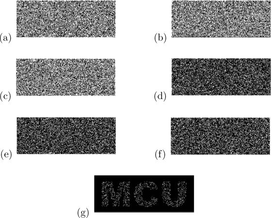
Implementation results of Algorithm 5 for VCRG-3 with respect to B: (a) $R_{1}^{5}$ $R_{1}^{5}$ , (b) $R_{2}^{5}$ $R_{2}^{5}$ , (c) $R_{3}^{5}$ $R_{3}^{5}$ ; (d) $R_{1}^{5} \otimes R_{2}^{5}$ $R_{1}^{5} \otimes R_{2}^{5}$ , (e) $R_{1}^{5} \otimes R_{3}^{5}$ $R_{1}^{5} \otimes R_{3}^{5}$ , (f) $R_{2}^{5} \otimes R_{3}^{5}$ $R_{2}^{5} \otimes R_{3}^{5}$ ; (g) $R_{1}^{5} \otimes R_{2}^{5} \otimes R_{3}^{5}$ $R_{1}^{5} \otimes R_{2}^{5} \otimes R_{3}^{5}$ .

Images

FIGURE 211.7
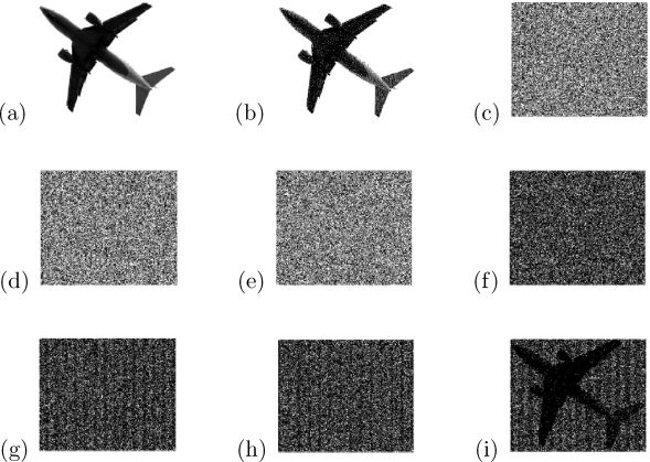
Implementation results of Algorithm 6 for VCRG-3 with respect to B: (a) $R_{1}^{6}$ $R_{1}^{6}$ , (b) $R_{2}^{6}$ $R_{2}^{6}$ , (c) $R_{3}^{6}$ $R_{3}^{6}$ ; (d) $R_{1}^{6} \otimes R_{2}^{6}$ $R_{1}^{6} \otimes R_{2}^{6}$ , (e) $R_{1}^{6} \otimes R_{3}^{6}$ $R_{1}^{6} \otimes R_{3}^{6}$ , (f) $R_{2}^{6} \otimes R_{3}^{6}$ $R_{2}^{6} \otimes R_{3}^{6}$ ; (g) $R_{1}^{6} \otimes R_{2}^{6} \otimes R_{3}^{6}$ $R_{1}^{6} \otimes R_{2}^{6} \otimes R_{3}^{6}$ .

Images

FIGURE 7.7
Results of Algorithm 7 where Encryption_VCRG (H, 3) was implemented by Algorithm 4 with respect to gray-level image G in Experiment 2: (a) G; (b) halftone version H of G; (c) $R_{1}^{4}$ $R_{1}^{4}$ , (d) $R_{2}^{4}$ $R_{2}^{4}$ , (e) $R_{3}^{4}$ $R_{3}^{4}$ ; (f) $R_{1}^{4} \otimes R_{2}^{4}$ $R_{1}^{4} \otimes R_{2}^{4}$ , (g) $R_{1}^{4} \otimes R_{3}^{4}$ $R_{1}^{4} \otimes R_{3}^{4}$ , (h) $R_{2}^{4} \otimes R_{3}^{4}$ $R_{2}^{4} \otimes R_{3}^{4}$ ; (i) $R_{1}^{4} \otimes R_{2}^{4} \otimes R_{3}^{4}$ $R_{1}^{4} \otimes R_{2}^{4} \otimes R_{3}^{4}$ .

Let ${R_{1}^{5}, R_{2}^{5}, R_{3}^{5}}$ ${R_{1}^{5}, R_{2}^{5}, R_{3}^{5}}$ and ${R_{1}^{6}, R_{2}^{6}, R_{3}^{6}}$ ${R_{1}^{6}, R_{2}^{6}, R_{3}^{6}}$ denote the outcomes of Algorithm 7 when Encryption_VCRG(H, 3) was implemented by Algorithms 5 and 6, respectively, with respect to G. Figures 7.8(a) and (b) are the superimposed results of $R_{1}^{5} \otimes R_{2}^{5} \otimes R_{3}^{5}$ $R_{1}^{5} \otimes R_{2}^{5} \otimes R_{3}^{5}$ and $R_{1}^{6} \otimes R_{2}^{6} \otimes R_{3}^{6}$ $R_{1}^{6} \otimes R_{2}^{6} \otimes R_{3}^{6}$ , respectively. It is noted that the three encrypted shares and the superimposed result of any group of two out of the three shares are indeed random grids that are omitted here.

The feasibility and applicability for Algorithm 7 to encrypt a gray-level image into VCRG-3 are demonstrated in a visual sense from Figures 7.7 and 7.8. Obviously, implementing Encryption_VCRG (H, 3) based upon Algorithm 4 makes Algorithm 7 achieve the highest contrast (while that based upon Algorithm 5 is the worst).

Experiment 3: Encrypting a color image to obtain color VCRG-3.

We tested Algorithm 8 with respect to a color image for obtaining color VCRG-3 in this experiment. Figure 7.9(a) is the color image P to be encrypted; (b), (c), and (d) are P^c, P^m, and P^y, which are the c, m, and y components of P, respectively; (e), (f), and (g) are P^c, P^m, and P^y which are the c-, m-, and y-colored halftone images (by error diffusion) of P^c, P^m and P^y, respectively.

Images

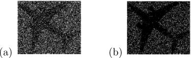
FIGURE 7.8
Reconstructed results of VCRG-3 with respect to G : (a) $R_{1}^{5} \otimes R_{2}^{5} \otimes R_{3}^{5}$ $R_{1}^{5} \otimes R_{2}^{5} \otimes R_{3}^{5}$ (b) $R_{1}^{6} \otimes R_{2}^{6} \otimes R_{3}^{6}$ $R_{1}^{6} \otimes R_{2}^{6} \otimes R_{3}^{6}$

By Step 3 of Algorithm 8, P^x would be encrypted into ${R_{1}^{x}, \otimes R_{2}^{x}, \otimes R_{3}^{x}}$ ${R_{1}^{x}, \otimes R_{2}^{x}, \otimes R_{3}^{x}}$ by Eycrypt_cVCRG(P^x, x, 3) for x ∈ {c, m, y}. When Eycrypt_cVCRG(P^m, m, 3) was based upon Algorithm 4, Figure 7.10 evidences the effectiveness of ${R_{1}^{m}, \otimes R_{2}^{m}, \otimes R_{3}^{m}}$ ${R_{1}^{m}, \otimes R_{2}^{m}, \otimes R_{3}^{m}}$ for being a set of m-colored VCRG-3 with respect to P^m in which (a)–(f) are the results of $R_{1}^{m}, R_{2}^{m}, R_{3}^{m}, R_{1}^{m} \otimes R_{2}^{m}, R_{1}^{m} \otimes R_{3}^{m}$ $R_{1}^{m}, R_{2}^{m}, R_{3}^{m}, R_{1}^{m} \otimes R_{2}^{m}, R_{1}^{m} \otimes R_{3}^{m}$ , and $R_{2}^{m} \otimes R_{3}^{m}$ $R_{2}^{m} \otimes R_{3}^{m}$ , respectively; and (g) is that of $R_{1}^{m} \otimes R_{2}^{m} \otimes R_{3}^{m}$ $R_{1}^{m} \otimes R_{2}^{m} \otimes R_{3}^{m}$ . Regarding P^c and P^y, the corresponding results are similar to Figure 7.10 so that we simply omit them.

The encrypted monochromatic-colored shares $P_{i}^{c}, P_{i}^{m}$ $P_{i}^{c}, P_{i}^{m}$ and $P_{i}^{y}$ $P_{i}^{y}$ were further composed to obtain color random grid $R_{i} = {P_{i}^{c}, P_{i}^{m}, P_{i}^{y}}$ $R_{i} = {P_{i}^{c}, P_{i}^{m}, P_{i}^{y}}$ for 1 ≤ i ≤ 3 in Step 4 of Algorithm 8. We show the corresponding results in Figure 7.11 where (a)–(c) are color random grids R₁, R₂, R₃; (d)–(f) give results of R₁ ⊗ R₂, R₁ ⊗ R₃, R₂ ⊗ R₃, respectively; and (g) shows that of R₁ ⊗ R₂ ⊗ R₃. When we implemented Eycrypt_cVCRG(P^x, x, 3) is based upon Algorithm 4, 5, or 6. The correctness of Theorem 4 holds in a visual sense from the results of Figures 7.8-10.

Experiment 4: Obtaining VCRG-4.

From the above analytic and experimental results, we know that Algorithm 4 achieves the higher light contrast as compared to Algorithms 5 and 6 for binary and gray-level images, so does Algorithm 8 based upon Algorithm 4 as compared to those based upon Algorithms 5 and 6 for a color image. We only tested Algorithm 4 for binary VCRG-4 and Algorithm 8 based upon Algorithm 4 for color VCRG-4 here. Figure 7.12 summarizes the results of binary VCRG-4 where (a) is the binary image B encrypted; (b)–(e) are R₁, R₂, R₃, R₄ produced by Algorithm 4; (f) presents the result of R₁ ⊗ R₂; (g) shows that of R₁ ⊗ R₂ ⊗ R₃; and (h) gives that of R₁ ⊗ R₂ ⊗ R₃ ⊗ R₄. Even though the superimposed results from other groups of less than four shares are not shown here, they are really random grids as expected. It is seen from Figure 7.12 that only when all four shares are superimposed can we see B, while no group of less than four shares tells anything about B. {R₁, R₂, R₃, R₄} is indeed a set of VCRG-4.

Images

FIGURE 214.7
(See color insert.) Results of Steps 1 and 2 of Algorithm 8 for VCRG-3 with respect to color image P in Experiment 3: (a) P; (b) P^c, (c) P^m, (d) P^y; (e) P^c, (f) P^m, (g) P^y.

Images

FIGURE 215.7
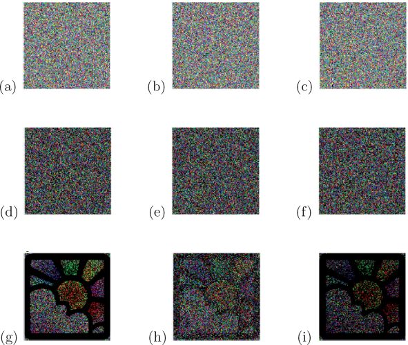
(See color insert.) Results of Step 3 of Algorithm 8 with respect to P^m where Eycrypt_cVCRG(P^m, m, 3) was based upon Algorithm 4: (a) $R_{1}^{m}$ $R_{1}^{m}$ , (b) $R_{2}^{m}$ $R_{2}^{m}$ , (c) $R_{3}^{m}$ $R_{3}^{m}$ ; (d) $R_{1}^{m} \otimes R_{2}^{m}$ $R_{1}^{m} \otimes R_{2}^{m}$ , (e) $R_{1}^{m} \otimes R_{3}^{m}$ $R_{1}^{m} \otimes R_{3}^{m}$ (f) $R_{2}^{m} \otimes R_{3}^{m}$ $R_{2}^{m} \otimes R_{3}^{m}$ (g) $R_{1}^{m} \otimes R_{2}^{m} \otimes R_{3}^{m}$ $R_{1}^{m} \otimes R_{2}^{m} \otimes R_{3}^{m}$ .

Images

FIGURE 216.7
(See color insert.) Results of Algorithm 8 for VCRG-3 with respect to P: (a) R₁, (b) R₂, (c) R₃; (d) R₁ ⊗ R₂, (e) R₁ ⊗ R₃, (f) R₂ ⊗ R₃; (g) R₁ ⊗ R₂ ⊗ R₃ (based upon Algorithm 4); (h) ${R^{'}}_{1} \otimes {R^{'}}_{2} \otimes {R^{'}}_{3}$ ${R^{'}}_{1} \otimes {R^{'}}_{2} \otimes {R^{'}}_{3}$ (based upon Algorithm 5); (i) ${R^{″}}_{1} \otimes {R^{″}}_{2} \otimes {R^{″}}_{3}$ ${R^{″}}_{1} \otimes {R^{″}}_{2} \otimes {R^{″}}_{3}$ (based upon Algorithm 6).

Images

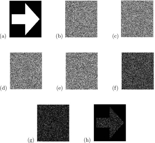
FIGURE 7.12
Results of Algorithms 4 for VCRG-4 with respect to binary image B: (a) B; (b) R₁, (c) R₂, (d) R₃, (e) R₄; (f) R₁ ⊗ R₂; (g) R₁ ⊗ R₂ ⊗ R₃; (h) R₁ ⊗ R₂; (g) R₁ ⊗ R₂ ⊗ R₃ ⊗ R₄.

Since n = 4 in this experiment, we have J(R_i) = 1/2 (see Figures 7.12(b)– (e)), J(R_i ⊗ R_j) = 1/4 (see (f)), and J(R_i ⊗ R_j ⊗ R_k) = 1/8 (see (g)) for 1 ≤ i ≠ j ≠ k ≤ 4. Further, from Table 7.6 we know that the light contrast of Algorithm 4 is c(ℰ₄) = 1/8 for n = 4. Figure 7.13 gives some experimental results of Algorithm 8 for color VCRG-4 where Eycrypt_cVCRG(P^x, x, 4) was based upon Algorithm 4 with respect to P (see Figure 7.9(a)). Figures 7.13(a)–(d) are the color random grids R₁, R₂, R₃, R₄ produced; (e) presents the result of R₁ ⊗ R₂; (f) shows that of R₁ ⊗ R₂ ⊗ R₃; and (g) gives that of R₁ ⊗ R₂ ⊗ R₃ ⊗ R₄. As seen from Figure 7.13, we realize that {R₁ ⊗ R₂ ⊗ R₃ ⊗ R₄} is a set of color VCRG-4 of P.

The results of the above four experiments are visualized evidences to the correctness of Theorems 2-4. The proposed schemes (Algorithms 4-8) in producing VCRG-n for a secret image are feasible and applicable. Among the approaches, Algorithm 4 (Algorithm 8 based upon Algorithm 4) is the most effective scheme in terms of light contrast for binary or gray-level (color) images.

Images

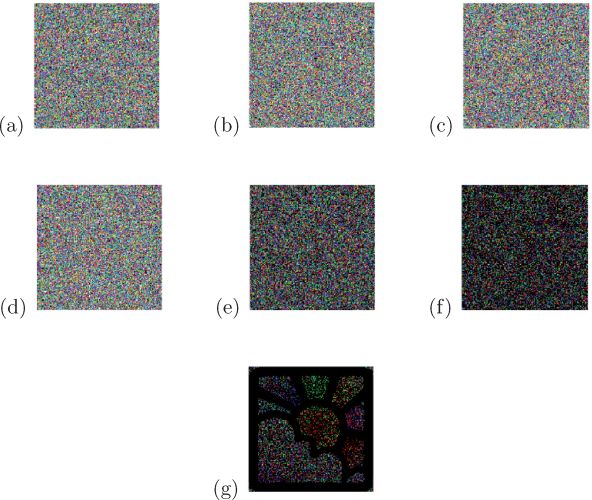
FIGURE 218.7
(See color insert.) Results of Algorithms 8 where Encrypt-cVCRG(P^x, x, 4) was based upon Algorithm 4 for VCRG-4 with respect to P (Figure 7.9(a)): (a) R₁, (b) R₂, (c) R₃, (d) R₄; (e) R₁ ⊗ R₂; (f) R₁ ⊗ R₂ ⊗ R₃; (g) R₁ ⊗ R₂ ⊗ R₃ ⊗ R₄.

It is noticed that when we adopt the light contrast to measure the reconstructed result for a conventional n out of n visual secret sharing scheme [9], the best result is 1/2ⁿ⁻¹. That means that Algorithm 4 achieves the same best light contrast. Moreover, it is so appealing that these schemes neither induce any extra pixel expansion nor require encoding basis matrix. Those approaches in conventional visual cryptography suffer from the disadvantage of the inevitable pixel expansion, which increases exponentially as n increases (and additionally increases as c or [log₂c] for the color cases where c is the number of colors in the secret image), in the basis matrices. Table 7.7 summarizes the pixel expansions needed by some efficient n out of n visual cryptographic schemes in the literature and our (n, n)-VCRG schemes. Owing to the reason that the size of the encrypted shares and reconstructed image would not be expanded, our schemes based upon random grids are more attractive than those in conventional visual cryptography for both theoretical concerns and practical applications.

Table7_7 Comparison of pixel expansions for conventional (n, n) visual cryptographic and (n, n)-VCRG schemes.

binary		color
Naor and Shamir [9]	Shyu [13]	Blundo et al. [3]	Shyu [11]	Shyu [13]
2ⁿ⁻¹	1	${\begin{matrix} (c - 1) 2^{n - 1} - c + 2 \\ if n is odd; \\ c (c - 1) 2^{n - 2} - c \\ otherwise \end{matrix}$ ${\begin{matrix} (c - 1) 2^{n - 1} - c + 2 \\ if n is odd; \\ c (c - 1) 2^{n - 2} - c \\ otherwise \end{matrix}$	[log₂c] × 2ⁿ⁻¹	1

7.4 Concluding Remarks

In this chapter, we propose novel schemes for visual secret sharing using random grids. At first, we give a new definition for the visual cryptograms of n(≥ 2) random grids with respect to a binary image. Based upon the definition, we design effective algorithms, prove their correctness formally, analyze the light contrast in the reconstructed image, and demonstrate their feasibility by computer simulations. By exploiting the skills of halftone and color decomposition in Ref. [12], the enhanced algorithms are also developed and verified to deal with gray-level and color images.

The proposed schemes incorporate human visual intelligence with information security in such a way that no computation but only human vision is needed in the decryption process. They provide cost effective, handy, and portable solutions to image encryption or sharing even for inexperienced users, especially for circumstances where no computer can be accessed. Since a secret image can be encrypted/shared among n(≥ 2) participants (instead of only two), our approaches extend and generalize the studies in Refs. [12, 7] such that the applicability of image encryption or sharing can be broadened to a greater extent.

The n shares of random grids generated by our VCRG-n algorithms work well just like those shares by the conventional n out of n visual secret sharing schemes based upon the definition of Naor and Shamir [9]. However, the pixel expansion in our schemes is 1 for both of the binary and color images, while that in Ref. [9] is 2ⁿ⁻¹ for the binary case and that in Ref. [11] is [log₂c] × 2ⁿ⁻¹ for the color image containing c colors. Therefore, the size of the encoded shares by our schemes would be much smaller (the same as the secret image). Further, the sophisticated encoding basis matrices in Refs. [9, 5, 4, 8, 14, 2, 1, 3, 10, 6, 11] are no more needed in our schemes. Regarding the visual perception in the reconstructed images, our Algorithm 4 achieves the same light contrast as good as the best n out of n visual secret sharing scheme devised in Ref. [9]. These clarify the superiority of our schemes.

Our encryption algorithms can be easily hardwired by incorporating a 0/1 random number generator with T flip-flops or Exclusive-OR gates. It would be an interesting challenge to design a special VCRG hardware for image encryption. In fact, many research topics in conventional visual cryptography could be reexamined in view of random grids.

Bibliography

[1] C.N. Yang and C.S. Laih. New colored visual secret sharing schemes. Des. Codes Cryptogr., 20:325–335, 2000.

[2] C. Blundo, A. De Santis, and D.R. Stinson. On the contrast in visual cryptography schemes. J. Cryptogr, 12:261–289, 1999.

[3] C. Blundo, A. De Santis, and D.R. Stinson. Improved schemes for visual cryptography. Des. Codes Cryptogr., 24:255–278, 2001.

[4] S. Droste. New results on visual cryptography. in: N. Koblitz (Ed.), Advances in Cryptology: CRYPTO96, Lecture Notes in Computer Science, 1109:401–415, 1996.

[5] G. Ateniese, C. Blundo, A. De Santis, and D. R. Stinson. Constructions and bounds for visual cryptography. in: F.M. der Heide, B. Monien (Eds.), Automata, Languages and Programming: ICALP’96, Lecture Notes in Computer Science, 1099, Springer, Berlin: 416–428, 1996.

[6] Y.C. Hou. Visual cryptography for color images. Pattern Recognition, 36:1619–1629, 2003.

[7] O. Kafri and E. Keren. Encryption of pictures and shapes by random grids. Opt. Lett, 12:377–379, 1987.

[8] M. Naor and B. Pinkas. Visual authentication and identification. in: B.S. KaliskiJr. (Ed.), Advances in Cryptology: CRYPTO97, Lecture Notes in Computer Science, 1294:322–336, 1997.

[9] M. Naor and A. Shamir. Visual cryptography. in: A. De Santis (Ed.), Advances in Cryptology: Eurpocrypt’94, Lecture Notes in Computer Science, 950:1–12, 1995.

[10] P.A. Eisen and D.R. Stinson. Threshold visual cryptography schemes with specified whiteness levels of reconstructed pixels. Des. Codes Cryptogr., 25:15–61, 2002.

[11] S.J. Shyu. Efficient visual secret sharing scheme for color images. Pattern Recognition, 39:866–880, 2006.

[12] S.J. Shyu. Image encryption by random grids. Pattern Recognition, 40:1014–1031, 2007.

[13] S.J. Shyu. Image encryption by multiple random grids. Pattern Recognition, 42:1582–1596, 2009.

[14] E.R. Verheul and H.C.A. Van Tilborg. Constructions and properties of k out of n visual secret sharing schemes. Designs Codes Cryptography, 11:179–196, 1997.

..................Content has been hidden....................

You can't read the all page of ebook, please click here login for view all page.

Table of Contents for
7 Visual Cryptography and Random Grids

7

Visual Cryptography and Random Grids

CONTENTS

7.1 Introduction

7.2 Random Grids

7.2.1 Random Pixel, Random Grid, and Average Light Transmission

7.2.2 Superimposition of Random Grids

7.3 Visual Cryptograms of Random Grids

7.3.1 Definition of VCRG

7.3.2 (2, 2)-VCRG Algorithms for Binary Images

7.3.3 Experiments for (2, 2)-VCRG

7.3.4 Definition of Light Contrast and Performance Evaluation

7.3.5 Algorithms of (n, n)-VCRG for Binary Images

7.3.6 Algorithms of (n, n)-VCRG for Gray-Level and Color Images

7.3.7 Experiments for (n, n)-VCRG

7.4 Concluding Remarks

Bibliography

Table of Contents for 7 Visual Cryptography and Random Grids

Create new playlist

Sign In

Sign Up

CONTENTS

Table of Contents for
7 Visual Cryptography and Random Grids