
13
Steganography in Halftone Images
Oscar C. Au, Yuanfang Guo and John S. Ho
Hong Kong University of Science and Technology, China
CONTENTS
13.1 Introduction
While gray-scale images can be readily displayed in computer monitors and other light-emitting displays, they also need to be displayed routinely in other reflective media such as newspaper, magazines, books, and other printed documents. However, in reflective media, the application of ink on the reflective media implies that only 1-bit images (with two tones: black and white) can be displayed. A problem arising from this is that straightforward 1-bit quantization on an image would lose most of the important image details. With such constraints, there is a class of image processing technique called image halftoning that converts an 8-bit image into an 1-bit image, which resembles the 8-bit image when viewed from a distance. Such 1-bit images are called halftone images [1]. Halftone image technologies are widely used in printed matters.
There are two main kinds of halftoning methods: ordered dithering [1] and error diffusion [2]. Ordered dithering uses straightforward 1-bit quantization with fixed pseudo-random threshold patterns to give halftone images with reasonable visual quality. Error diffusion also performs simply 1-bit quantization but allows the 1-bit quantization error to be fed back to the system and thus can achieve higher visual quality than ordered dithering.
Sometimes it is desirable to hide watermarking data in halftone images. Some halftone image watermarks are designed to be fragile and are useful for authentication and tamper detecting of the halftone images. Some halftone image watermarks are designed to be robust and are useful for copyright protection. In some applications, the data are to be embedded into a single halftone image and some special method can be used to read the hidden data. In other applications, visual patterns are hidden in two or more halftone images such that, when they are overlaid, the hidden visual patterns can be revealed. This kindly visual pattern hiding is also called visual cryptography. This chapter is about visual cryptography in error diffused halftone images.
The chapter is organized as follows. Section 13.2 introduces the basic error diffusion technique. Section 13.3 introduces a visual cryptography method for error diffused images called Data Hiding by Stochastic Error Diffusion (DHSED) [3]. Section 13.4 introduces an improved method called Data Hiding by Conjugate Error Diffusion (DHCED) [4]. Section 13.5 gives theoretical and empirical analysis of DHSED and DHCED. At last, Section 13.6 will give a summary of this chapter.
13.2 A Review of Error Diffusion
In this section, we will briefly introduce a halftoning method called Error Diffusion. The method that we will describe is by no means the only way to achieve halftoning, but is a popular approach that gives good visual quality while maintaining reasonable complexity. The error diffusion process converts a multitone image to a halftone one by distributing the error introduced at the current pixel to a neighborhood of yet unprocessed pixels. The neighborhood, as well as the weights in the distribution, is described by a set of positions and weights known as an error kernel. This diffusion of error across a region allows the local intensity of the halftone image to be preserved approximately.
Consider a multitone image with pixels defined over the range of 0 (black) to 255 (white). Let h(k, l) be an error kernel defined over a neighborhood N. For example, the common Steinberg kernel [2] is
defined over the neighborhood N = {(0,1), (1, – 1), (1,0), (1,1)}. Here we have used * to indicate the location of the current pixel. Let (i, j) be the current pixel location. Let x(i, j) be the current multitone pixel to be processed. A modified pixel value u(i, j) will be derived from x(i, j) and 1-bit quantization is applied to u(i, j) to give the output halftoned pixel value y(i, j). Let e(i, j) be the error between u(i, j) and y(i, j). In error diffusion, the error e(i, j) is distributed to future pixels in its neighborhood. For the case of error diffusion using the Steinberg kernel, a portion of e(i, j) will be distributed to (i, j + 1) corresponding to (0,1) in N. Similarly, of e(i, j) goes to (i + 1, j – 1), of it goes to (i + 1, j), and of it goes to (i + 1, j + 1).
For location (i, j), an offset term a(i, j) is defined as
which is the total error propagated from past pixels to the current pixel. For the error at location (i – k, j – l), a portion h(k, l) of it is passed to the current pixel according to the error kernel. The modified pixel value u(i, j) is then defined as
The output halftone value y(i, j) is defined as
and the error e(i, j) is
These steps are summarized in Figure 13.1, in which the block Q(·) is the 1-bit quantization and the block hk,l is the error kernel applied to past errors in the neighborhood to generate the current offset a(i, j).
Consider the special case of X being of constant intensity A in a neighborhood around (i, j). As error diffusion can preserve the average image intensity, the probability distribution of a halftone pixel y(i, j) is
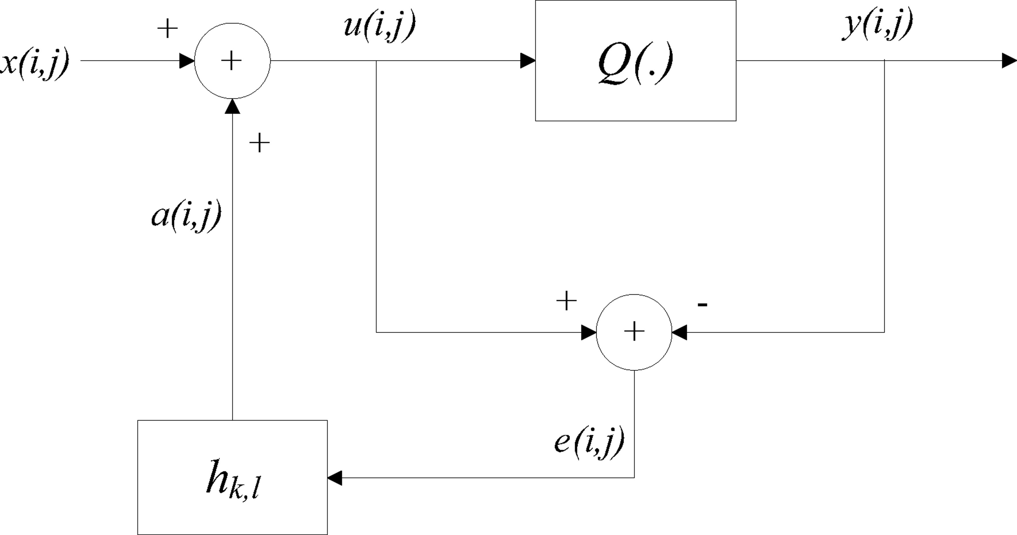
FIGURE 13.1
Error diffusion process.
such that
Typically, the percentages of white and black pixels in X are A/255 • 100% and (255 – A)/255 • 100% respectively, distributed evenly in X. In a way, one can argue that
such that
Another common error diffusion kernel is the Jarvis kernel [5]

FIGURE 13.2
Original multitone ”Lena” (X).

FIGURE 355.13
Halftone image generated by error diffusion with the Steinberg kernel.

FIGURE 13.4
Halftone image generated by error diffusion with the Jarvis kernel (Y1).
which has a larger support than the Steinberg kernel. A typical image, Lena, is shown in Figure 13.2. The corresponding halftone images generated by Steinberg and Jarvis kernels are shown in Figures 13.3 and 13.4 respectively. It can be observed that different error diffusion kernels give rise to different textures in the halftone images. In general, Jarvis gives images with higher contrast while the Steinberg kernal gives smoother texture. Both are capable of generating halftone images that mimic the original images when viewed afar, though tiny details of the original image such as Lena’s hair tend to be masked by the halftone image texture generated by the error kernel.
The size of all the images in this chapter are 512 × 512. Due to limited space, all remaining halftone figures are generated by the Jarvis kernel only, though the methods described in the chapter are applicable to any error diffusion kernels.
13.3 Data Hiding by Stochastic Error Diffusion (DHSED)
Data Hiding for halftone images is quite different from that for multitone images due to the fact that halftone pixels can take on only two values: 0 and 255. They contain high frequency noise but resemble the original multitone images when viewed afar. As such, normal data hiding techniques such as least significant bit (LSB) embedding technique [6] would not work on them because the resulting stego-images will be effectively the watermark image and would not resemble the original multitone images even when viewed afar. Thus, it is necessary to develop special data hiding techniques for halftone images. Although several data hiding technologies for halftone images have been proposed before, Data Hiding by Stochastic Error Diffusion (DHSED) is the first visual cryptography method based on error diffusion.
DHSED is a method that embeds a binary secret pattern into two halftone images derived from the same underlying multitone image. The binary pattern should be revealed when the two halftone images are superimposed. The idea of DHSED is to stochastically create a texture phase shift between the two halftone images at locations where the watermark is ”active” or black (binary pattern value being zero). The resulting mismatch allows the watermark to become visible while maintaining the original halftone background. Let X be the original multitone image and W the binary secret pattern of the same size. Let Y1 be a halftone image obtained by applying regular error diffusion to X. Let Y2 be the halftone image obtained through DHSED. The problem, then, is to obtain Y2 such that W is revealed when Y1 and Y2 are overlaid. We denote the individual pixels at location (i, j) of both halftone images as y1(i,j) and y2(i,j), respectively.
The second image Y2 is generated by applying regular error diffusion to certain areas in X, but with different error conditions. These areas are obtained by referencing both Y1 and W. Let Wb be the collection of the locations of all the black pixels in W, and Ww the collection of the white pixel locations. In constructing Y2, we will force the pixel value at all locations belonging to Ww to be identical to Y1. In other words, values at these locations are merely copied from Y1 to Y2. That is,
For the remaining pixels in Wb, Y2 needs to look natural and thus DHSED applies error diffusion with the same error kernel. However, DHSED seeks to make Y2 different from Y1 statistically so that when they are overlaid, pixels in Wb would tend to be darker. To achieve this, DHSED first morphologically dilate, Wb with a structuring element D consisting of a (2L +1) × (2L + 1) matrix. We denote the dilated Wb as C.
which can be interpreted as a L-pixel expansion of Wb in all directions.
For the pixels outside C, DHSED copies Y2 from Y1 using (13.10) but forces the error for Y2 to be zero, i.e. e2(i, j) = 0 for (i, j) ∉ C. Note that the error for Y1 are nonzero in general for the same locations.
Let E = C – Wb = C ∩ Ww be the ”border” of the secret pattern, obtained by removing Wb from the expanded region C. For the pixels in E, (13.1) and (13.2) are still applied while (13.3) and (13.4) are not. (13.10) will be used to replace (13.3) since E ⊂ Ww and Y2 pixels in Ww are copied from Y1. We will use (13.12) to replace (13.4).
which is basically (13.4) with a limiter. As Y2 pixels in E are copied from Y1 with artificial zero error outside C, there are chances that u2(i, j) – y2(i, j) is outside ± 127. The limiter would then help to make the e2(i, j) reasonable.
For the pixels in Wb, DHSED uses regular error diffusion to generate Y2 so that region Wb in Y2 still has the same characteristic texture as regular error diffusion. But the ”phase” of the texture will be different compared to the corresponding region in Y1 since the error outside the region C is different in Y1 and Y2.
The overlaying operation is equivalent to applying the logical AND operation between images Y1 and Y2. Since the pixels in region Ww of Y1 and Y2 have been forced to be identical, the overlaid pixel values are simply the regular error diffused pixel values. However, in region Wb, although the texture in Y1 and Y2 maintains the same characteristic, there is an artificially introduced phase shift such that collocated Y1 and Y2 pixels tend to be statistically independent. As a result, the overlaying operation tends to give darker local intensity thus revealing the secret pattern W. A more detailed analysis of this will be given in Section 13.4.
Using Lena as the test image and Figure 13.5 as the secret binary pattern W, Figure 13.4 is Y1 and Figure 13.6 is Y2 generated using DHSED with respect to Y1 and W. A threshold L = 5 is used. Note that Figure 13.6 looks like Figure 13.4, which verifies that DHSED can give halftone images with good visual quality. Figure 13.7 shows the image obtained by overlaying Figure 13.6 and Figure 13.4. The secret pattern W is clearly visible in Figure 13.7 verifying that DHSED is an effective visual cryptography method.

FIGURE 13.5
Secret pattern ”UST” to be embedded in the halftone image (W).

FIGURE 13.6
DHSED-generated Y2 (L = 5) of Lena with respect to X in Figure 13.2, W in Figure 13.5, and Y1 in Figure 13.4.

FIGURE 359.13
Image Y obtained by overlaying Y1 in Figure 13.4 and Y2 in Figure 13.6.
13.4 Data Hiding by Conjugate Error Diffusion (DHCED)
DHSED as outlined in the previous section is both computationally and conceptually simple, but suffers from three major problems. First, Y1 and Y2 must be obtained from the same X. In other words, DHSED cannot embed a binary secret pattern in two halftone images obtained from two different multitone images. Second, when the images are overlaid, the contrast of the revealed secret pattern is relatively low. Third, occasional boundary artifacts may happen in Y2 especially towards the right and bottom sides of the secret pattern where error is not diffused properly across the Wb boundary. Such boundary artifacts can lower the visual quality of Y2 considerably.
In this section, we will introduce another method called Data Hiding by Conjugate Error Diffusion (DHCED) that addresses these three problems.

FIGURE 360.13
The DHCED (Data Hiding by Conjugate Error Diffusion) process.
The block diagram of DHCED is shown in Figure 13.8. Unlike DHSED, the problem now contains two original multitone images X1 and X2, where X1 and X2 may or may not be identical. Two halftone images Y1 and Y2 are to be generated from X1 and X2, respectively such that when Y1 and Y2 are overlaid, the binary secret pattern W is revealed. Similar to DHSED, Y1 is generated using regular error diffusion on X1. Then the DHCED process in Figure 13.8 is used to generate Y2.
To explain the detailed operation of DHCED, we assign logical ”1” to pixel value 255 and logical ”0” to pixel value 0. The conjugate of a pixel is then equivalent to logical NOT, or toggling of the value. Recall that Ww and Wb are the collections of white and black pixel locations in W, respectively. As Y1 is already generated by regular error diffusion, the secret pattern W at location (i, j) can be naively inserted in Y2 as follows
where (·)c denotes logical NOT. This is equivalent to logical XNOR between Y1 and W. The resulting Y2 will look like X1 in Ww and the negative of X1 in Wb because
But Y2 should resemble X2 instead of X1 and thus this naive method does not work. Even if X1 and X2 are the same image, this naive method does not work in Wb as Y2 should resemble X1 instead of the negative of X1.
Although this naive method does not work, DHCED follows a similar logic except that it favors, instead of forces, Y2 to take on the values in (13.13). In other words, it treats the value in (13.13) as the favored value of y2(i, j).
Consider Figure 13.8 and any location (i, j) ∈ Wb. Basically, DHCED applies error diffusion on x2(i, j) including (13.1) to calculate α2(i, j), (13.2) to calculate u2(i,j) and, in the first Q(·) block, (13.3) to calculate the trial halftone value y2(i, j). In the N(·) block, the trial value is compared with the favored value that is obtained by XNOR of w(i, j) and y1(i, j). If they are equal, no change needs to be done to x2(i, j) and u2(i, j) such that u′2(i, j) = u2(i, j). If they are not equal, DHCED considers the possibility of forcing trial y2(i, j) to toggle to achieve the favored value. Recognizing that forced toggling is equivalent to applying a distortion to x2(i, j) followed by regular error diffusion, DHCED will execute the forced toggling only if the required distortion is not excessive.
Here are the details. Note that forcing the trial halftone value to toggle is equivalent to adding an offset value Δu(i, j) to u2(i, j). If the trial value should be toggled from 0 to 255, then u2(i, j) < 128 initially and we need an offset Δu(i, j) such that the resulting value, which we called u′2(i, j), is u2(i, j) ≡ u2(i,j) + Δu(i, j) ≥ 128. Thus, there is a lower bound for Δu(i, j): Δu(i, j) ≥ 128 – u2(i, j) > 0.
Likewise, if we want to toggle from 255 to 0, then u2(i, j) ≥ 128 initially and we need an offset Δu(i, j) such that u′2(i, j) ≡ u2(i, j) + Δu(i, j) ≤ 127. There is thus an upper bound for Δu(i, j): Δu(i, j) ≤ 127 – u2(i, j) < 0.
The smallest Δu(i, j) (in terms of magnitude) needed to achieve toggling is
We further note that adding a distortion Δu(i, j) to u2(i,j) may be interpreted as a distortion to the original multitone image pixel x2(i, j). Defining Δx(i, j) = Δu(i, j), the input to the normal quantizer u′2(i, j) may be written as
The interpretation of (13.18) is that the output halftone image using DHCED in fact represents , not X2, in the sense of that it can be obtained from directly using standard error diffusion. Thus, |Δx| can be treated as a measure of the distortion introduced by the DHCED process. To control this distortion, we define a threshold T that determines whether or not the pixel should be toggled, allowing a trade-off between distortion and visual quality of the watermarked halftone image. If |Δx| is less than T, the pixel toggling will be performed, and vice versa. If T decreases, the visual quality of the watermarked image Y2 will improve at the price of lower contrast of the secret pattern when the two halftone images are superimposed.
Consider any location (i, j) ∈ Ww. If X1 and X2 are the same image, DHCED would copy y1 (i, j) to y2 (i, j) so that Y2 values are effectively obtained by applying error diffusion to X1. The error e2 (i, j) will be computed as in normal error diffusion. When Y1 and Y2 are overlaid, the regular error diffused value y1(i, j) will be revealed. The overlaying operation will reveal a local intensity similar to the local intensity of X1, which is typical for regular error diffusion.
If X1 and X2 are different, DHCED would not force y2(i, j) to be identical to y1(i, j) at (i, j) ∈ Ww. Instead, it merely treats y1(i, j) as the favored value of y2(i, j). And DHCED performs the same operation as in Wb.
The proposed DHCED for the case of identical X1 and X2 is simulated. Using Lena as the test image and Figure 13.5 as the secret binary pattern W, Figure 13.4 is Y1 and Figure 13.9 is Y2 generated using DHCED with respect to Y1 and W. A threshold of T – 10 is used. Note that Figure 13.9 looks like Figure 13.4 which verifies that DHCED can give halftone images with good visual quality. Figure 13.10 shows the image obtained by overlaying Figure 13.9 and Figure 13.4. The secret pattern W is clearly visible in Figure 13.7 verifying that DHSED is an effective visual cryptography method.

FIGURE 363.13
DHCED-generated Y2 (T = 10) of Lena with respect to X in Figure 13.2, W in Figure 13.5, and Y1 in Figure 13.4.
Comparing DHSED and DHCED, it can be observed that DHSED in Figure 13.6 has strong boundary artifacts along the embedded watermark especially on the right and bottom edges of W. With DHCED, the boundary artifacts are reduced considerably. In addition, the watermark in Figure 13.10 is significantly more visible than Figure 13.7 in terms of contrast, when Y1 and Y2 are overlaid.
DHCED for the case of different X1 and X2 is also simulated. Here Lena is used as X1 and Pepper is used as X2. The Y1 with respect to X1 is simply the one in Figure 13.4. The DHCED generated Y2 from X2 with respect to Y1 and W is shown in Figure 13.12. A threshold of T = 10 is used. The overlaid image of Y1 and Y2 is shown in Figure 13.13. As expected, traces of both Lena and Pepper can be observed in the overlaid image. More importantly, the watermark W is revealed also, though the contrast of W in Figure 13.13 is not as good as in Figure 13.10.
13.5 Performance Analysis
In this section, we give an indepth analysis of both DHSED and DHCED. We will show theoretically why DHCED has better performance than DHSED.

FIGURE 364.13
Image Y obtained by overlaying Y1 in Figure 13.4 and Y2 in Figure 13.9.

FIGURE 13.11
Original multitone ”Pepper” (X2).

FIGURE 365.13
DHCED-generated Y2 (T = 10) of Pepper with respect to X2 in Figure 13.11, W in Figure 13.5, and Y1 in Figure 13.4.

FIGURE 13.13
Image Y obtained by overlaying Y1 in Figure 13.4 and Y2 in Figure 13.12.
Consider the case when X1 and X2 are the same image X. Consider a rectangular region R of constant intensity A in X. Suppose that the left half of R is in the white region Ww of W and the right half in the black region Wb of W. We assume that error diffusion is effective in both the left and right halves of R such that the average image intensity is preserved. Thus, the probability distribution of a halftone pixel y1 (i, j) in the region R of Y1 is
such that the expected value is
for (i, j) ∈ R. Typically, the percentage of white and black pixels in Y1 in R are A/255 • 100% and (255 – A)/255 • 100% respectively, distributed evenly in R.
The generation of Y2 using DHCED is effectively the application of error diffusion to the equivalent noisy multitone image. And the error diffusion should be effective, as usual. The distortion Δx(i, j) introduced by DHCED is equally likely to be positive and negative and its magnitude is bounded by T. The average intensity in R should still be approximately A. Thus, the probability distribution of a halftone pixel y2(i, j) in the region R of Y2 is approximately
such that
for (i, j) ∈ RA.
Let y(i, j) = y1(i, j) ∩ y2(i, j) be the output pixel obtained by overlaying Y1 and Y2. The y(i, j) would be white only if both y1(i, j) and y2(i, j) are white. For the proposed DHCED, the y1(i, j) and y2(i, j) are designed to be dependent.
In the left half of R, which is in Ww, DHCED would simply copy y1(i, j) as y2(i, j) such that P[y2(i, j) = y1(i, j)] = 1. Then
such that
In other words, y(i, j) = y1(i, j)) = y2(i, j) for the region Ww and the overlay operation does not change the halftone pixel values at all.
In the right half of R which is in Wb, the y1(i, j) and y2(i, j) are favored to be conjugate to each other (y2(i, j) ≈ y1(i, j)) such that y1(i, j) and y2(i, j) tend not to be black at the same time. To investigate the behavior of y(i, j), we consider two different cases: (1) 255 ≥ A > 127 and (2) 127 ≥ A ≥ 0.
For the case of 255 ≥ A > 127, there are more white pixels than black pixels in R of Y1. The percentage of black pixels in the right half of R of Y1 is about (255 – A)/255 • 100%. For example, if A = 190, about 25% of the pixels in the right half of R of Y1 should be black. As y1(i, j) and y2(i, j) tend not to be black at the same time, the black pixels in the right half of R of Y2 tend to be at different locations from those in Y1. Consequently, the percentage of black pixels in the right half of R of Y tends to be doubled to 2 • (255 – A)/255 • 100%. In our example of A = 190, the approximately 25% black pixels in the right half of R of Y1 and those of Y2 tend to be at different locations such that there are about 50% black pixels in the right half of R of Y. Thus,
such that
In other words, the expected value should increase approximately linearly with A, from 1 (for A = 128) to 255 (for A = 255). The difference between the average intensity of the left and right halves of R for 255 ≥ A > 127 is
For the case of 127 ≥ A ≥ 0, there are fewer white pixels than black pixels in the right half of R of Y1. Again the y1(i, j) and y2(i, j) tend not to be black at the same time in DHCED. This implies that the black pixels in the right half of R of Y2 tend to fill up all the white pixel locations in the right half of R of Y1, leading to all y(i, j) being black. Thus, P(y(i, j) = 0) ≈ 1 and
for 127 ≥ A ≥ 0. And the difference between the average intensity of the left and right halves of R is, for 127 ≥ A ≥ 0,
Consequently, the contrast between the left and right halves of R of Y can be expressed as, for 255 ≥ A > 127,
and, for 127 ≥ A ≥ 0,
To summarize, for any (i, j) in the right half of R that is in Wb, the expected value of y(i, j) is
The difference in average intensity of the left half and right half of R is
and the contrast between the left half and right half of R is
To verify these, we simulate DHCED using an artificial image called ”Ramp” shown in Figure 13.14 as X = X1 = X2, in which the image intensity decreases gradually and linearly from 255 at the top row to 0 at the bottom row. The hidden pattern to be embedded is called ”Column” and is black at the center and white on the left and right, as shown in Figure 13.15. The DHCED generated Y1 and Y2 are shown in Figures 13.16 and 13.17, respectively. The row-wise average intensity of Y1 and Y2 are plotted against the average intensity of the corresponding row in X in Figure 13.22. As expected, the row-wise average intensity of Y1 and Y2 are very similar to the corresponding intensity in X, which verifies (13.21) and (13.24).
Figure 13.18 is the overlaid image Y. We note that in the Ww region, Y is identical to Y1 and Y2, with intensity decreasing from top to bottom. In the Wb region, the intensity of Y is as high as X at the top. But as the intensity of X decreases from the top to bottom, we observe that the intensity of Y decreases at a fast pace to about the middle of the image (where intensity is about 127), and remains low in the lower half of the image.
To show the exact behavior of Y in the Wb region, we compute the average intensity in the Wb for each row of Y and plot it against the average intensity of the corresponding row in X in Figure 13.19. Three such curves are obtained with 3 values of T, namely T = 5, 10, 15. Also shown in the figure is the theoretical behavior as predicted by (13.35). It can be observed from the figure that as T increases, the average intensity curves appear to converge to the theoretical curve, as expected.

FIGURE 13.14
Original multitone image ”Ramp” (X).

FIGURE 13.15
Secret pattern ”Column” to be embedded in the halftone image (W).

FIGURE 370.13
Halftone images generated by error diffusion with the Jarvis kernel (Y1).
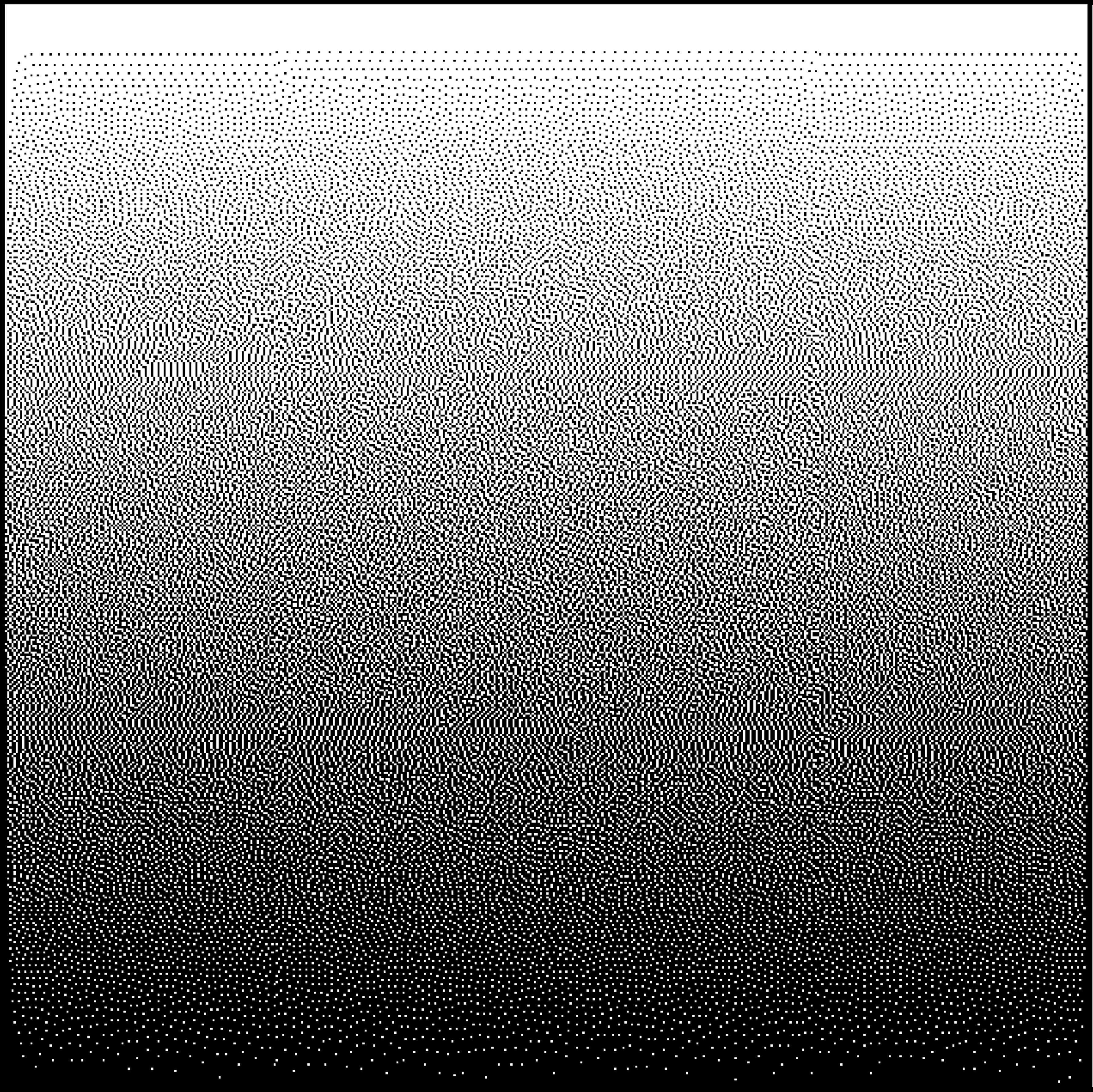
FIGURE 13.17
DHCED-generated Y2 (T = 10) of Ramp with respect to X in Figure 13.14, W in Figure 13.15, and Y1 in Figure 13.16.

FIGURE 371.13
Image Y obtained by overlaying Y1 in Figure 13.16 and Y2 in Figure 13.17.
We also compute the difference between the average intensity in the W5 and the Ww regions for each row of Y, and plot this Δintensity against the average intensity of the corresponding row in X in Figure 13.20. Similarly, the contrast is computed and plotted in Figure 13.21. Also shown in the two figures are the theoretical behavior predicted by (13.36) and (13.37). It can be observed that as T increases, the Δintensity curves and the contrast curves appear to converge to the corresponding theoretical curves, as expected.
Next, we analyze DHSED and make a comparison with DHCED. Since DHSED forces Y1 and Y2 to be identical in Ww, both y1(i, j) and y2(i, j) are identical in the left half of R and the probability distribution is
such that E[y(i, j)] = A. For any (i, j) in Wb, the corresponding pixel values in Y1 and in Y2 are error diffused with relative random phase. Thus, the local intensity for Y1 and Y2 is

FIGURE 372.13
Row-wise average intensity of Wb in Y in Figure 13.18 vs row-wise average intensity of X in Figure 13.14 (Ramp).

FIGURE 13.20
Row-wise Δintensity of Y in Figure 13.18 vs row-wise average intensity of X in Figure 13.14 (Ramp).
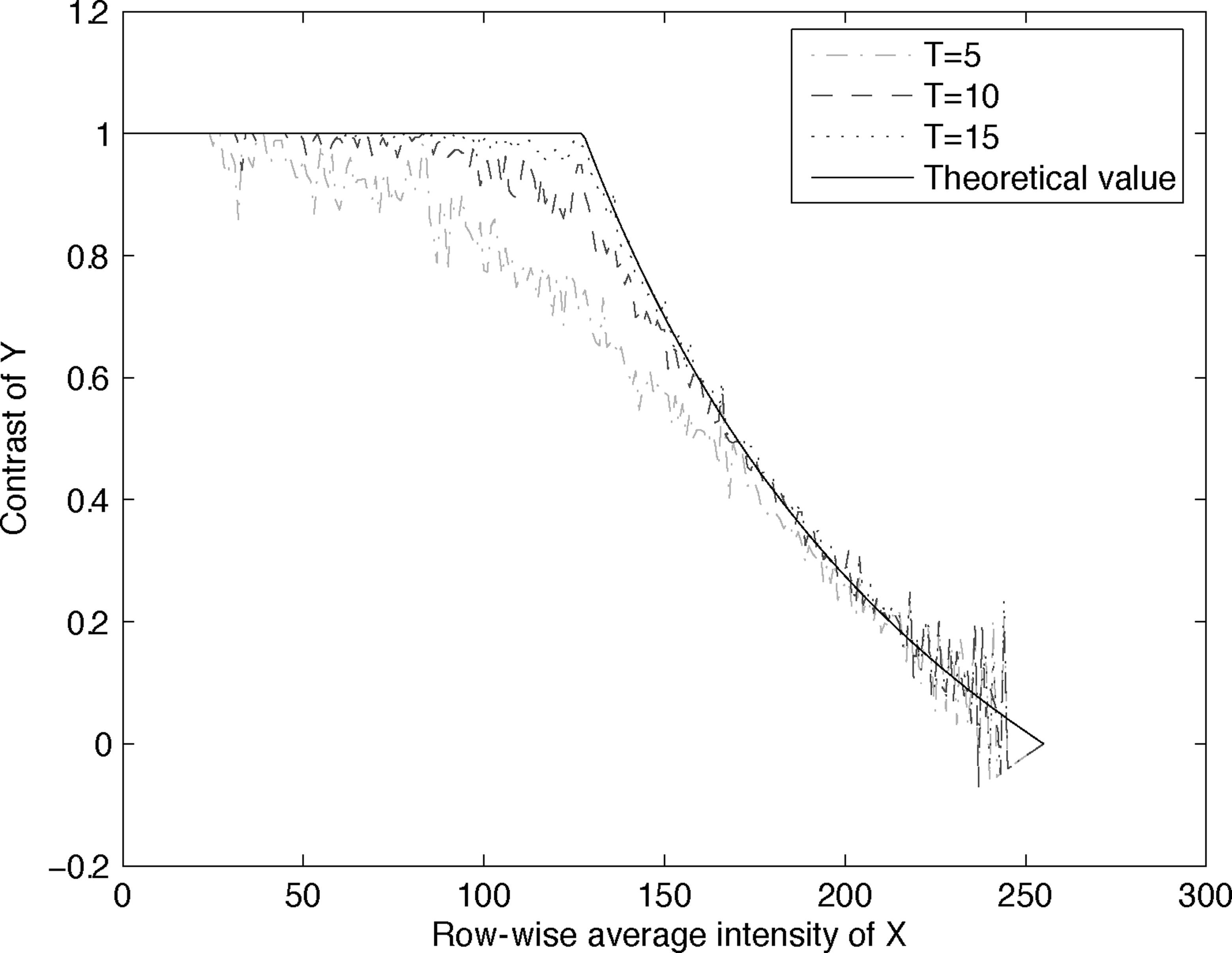
FIGURE 373.13
Contrast of Y in Figure 13.18 vs row-wise average intensity of X in Figure 13.14 (Ramp).
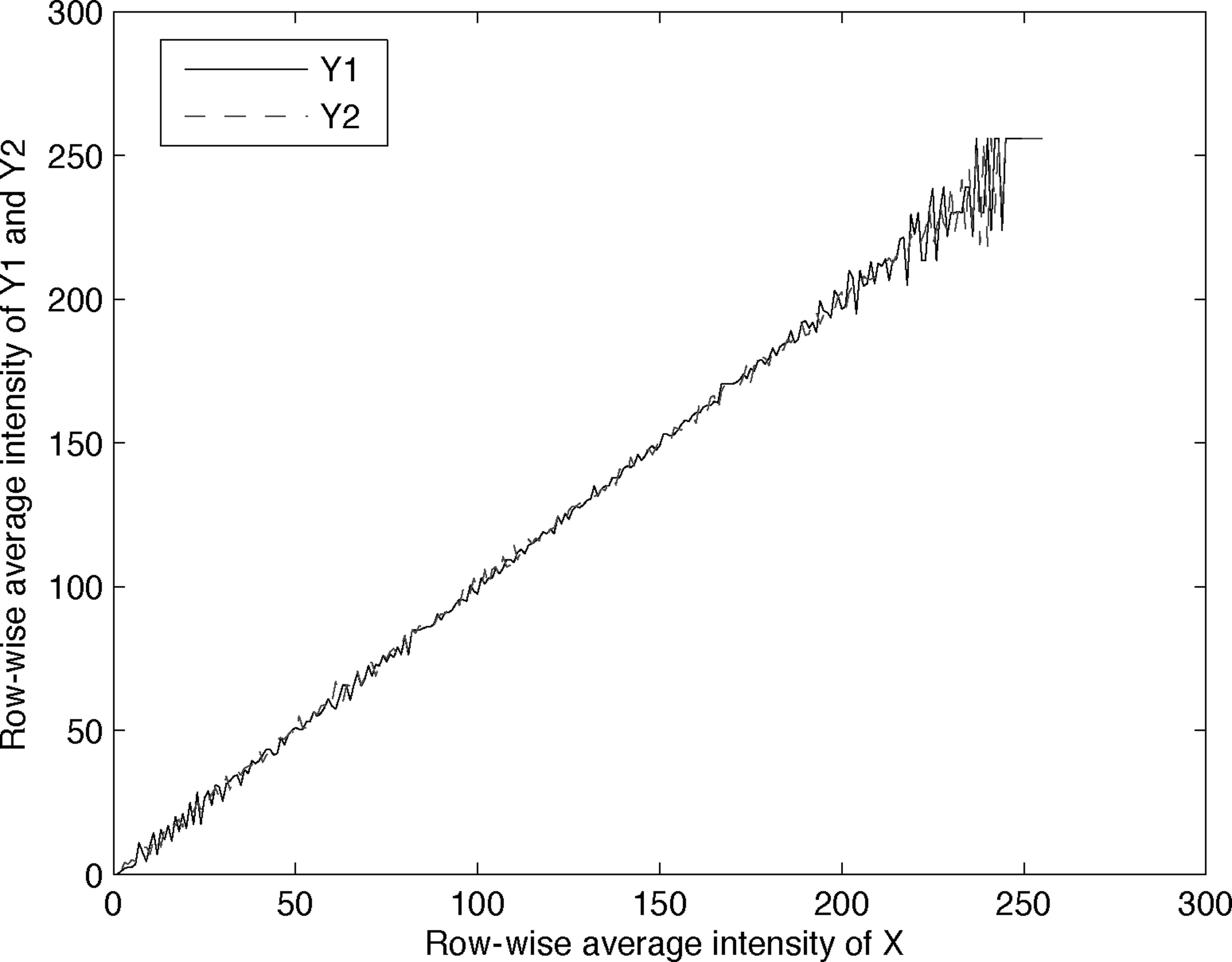
FIGURE 13.22
Row-wise average intensity of Y1 in Figure 13.4 and Y2 in Figure 13.9 vs row-wise average intensity of X in Figure 13.14 (Ramp).
and y1(i, j) and y2(i, j) are approximately independent with
such that
Thus, the intensity of DHSED is expected to be greater than or equal to that of DHCED, with equality if A = 255. The difference in average intensity is
The contrast is
We also simulate DHSED on Ramp to verify the equations above. The hidden pattern is still the Column in Figure 13.15. The DHSED generated Y1 and Y2 are shown in Figures 13.16 and 13.23, respectively. In Figure 13.28, the row-wise average intensity of Y1 and Y2 are plotted against the average intensity of the corresponding row in X. As expected, they are very similar to X, which verifies (13.39).
Figure 13.24 is the overlaid image Y. Similar to DHCED, the Y of DHSED is identical to Y1 and Y2 in the Ww region, with intensity decreasing from top to bottom. In the Wb region, the intensity of Y is as high as X at the top row. But as the intensity of X decreases towards the bottom of the image, the intensity of Y decreases faster in the center than on the two sides. In other words, the intensity of Y decreases faster in Wb than in Ww, making Wb visible in Y.
Similar to DHCED, to show the exact behavior of DHSED in Wb in Y, we compute the average intensity in the Wb for each row of Y and plot it against the average intensity of the corresponding row in X in Figure 13.25. Three curves are obtained for 3 values of L, namely L = 1, 5, 10. Also shown is the theoretical curve according to (13.42). It can be observed that the 3 empirical curves match the theoretical curve very well. This also suggests that the choice of L does not have much effect on the intensity of Wb in Y.
We also compute the difference between the average intensity in Wb and Ww regions for each row of Y, and plot this Δintensity against the average intensity of the corresponding row in X in Figure 13.26. Similarly, the contrast is computed and plotted in Figure 13.27. Also shown in the two figures are the theoretical behavior predicted by (13.43) and (13.44). It can be observed that the empirical Δintensity curves and contrast curves are similar to the corresponding theoretical curves, as expected. Again, the choice of L has little effect.
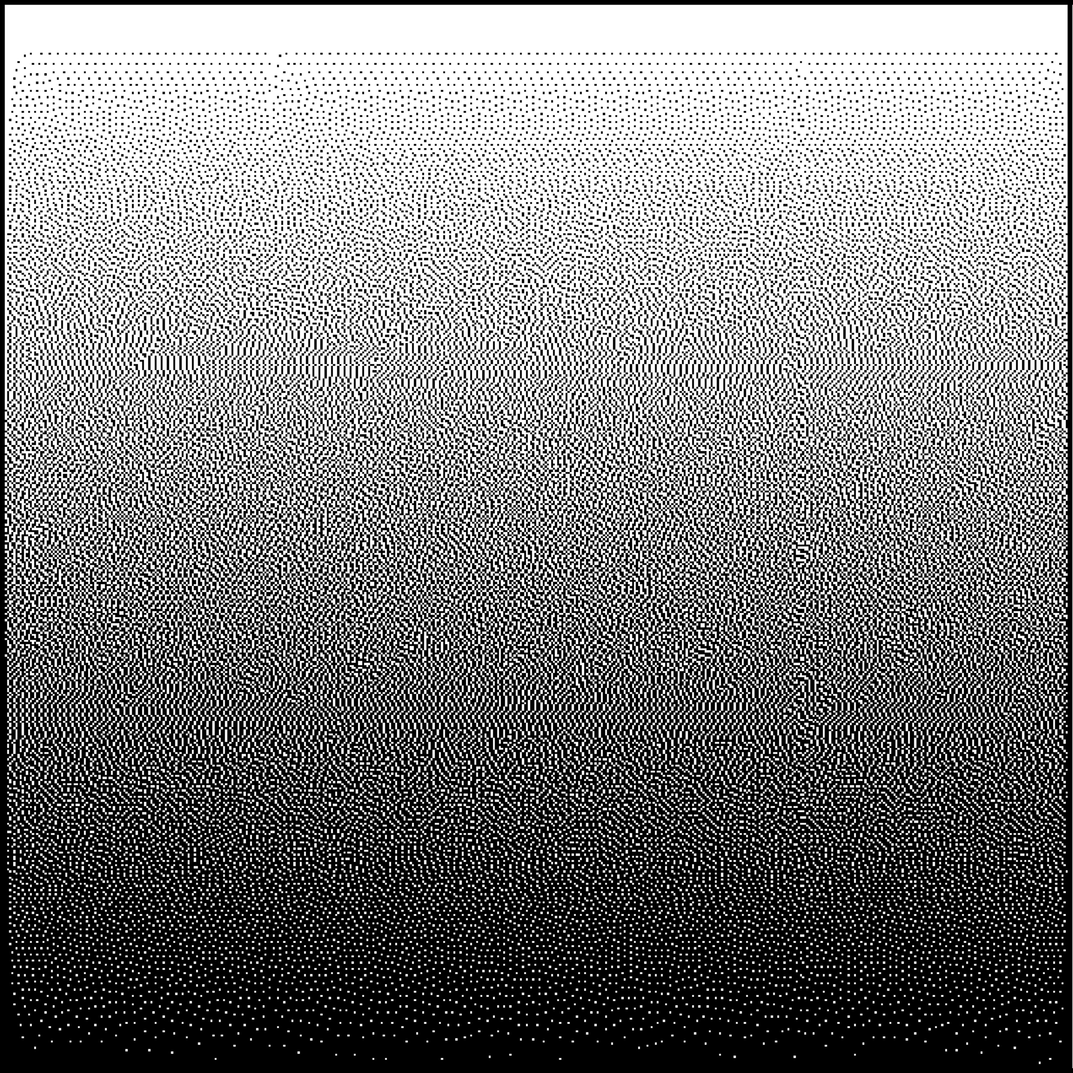
FIGURE 13.23
DHSED-generated Y2 (L = 5) of Ramp with respect to X in Figure 13.14, W in Figure 13.15 and Y1 in Figure 13.16.

FIGURE 13.24
Image Y obtained by overlaying Y1 in Figure 13.16 and Y2 in Figure 13.23.
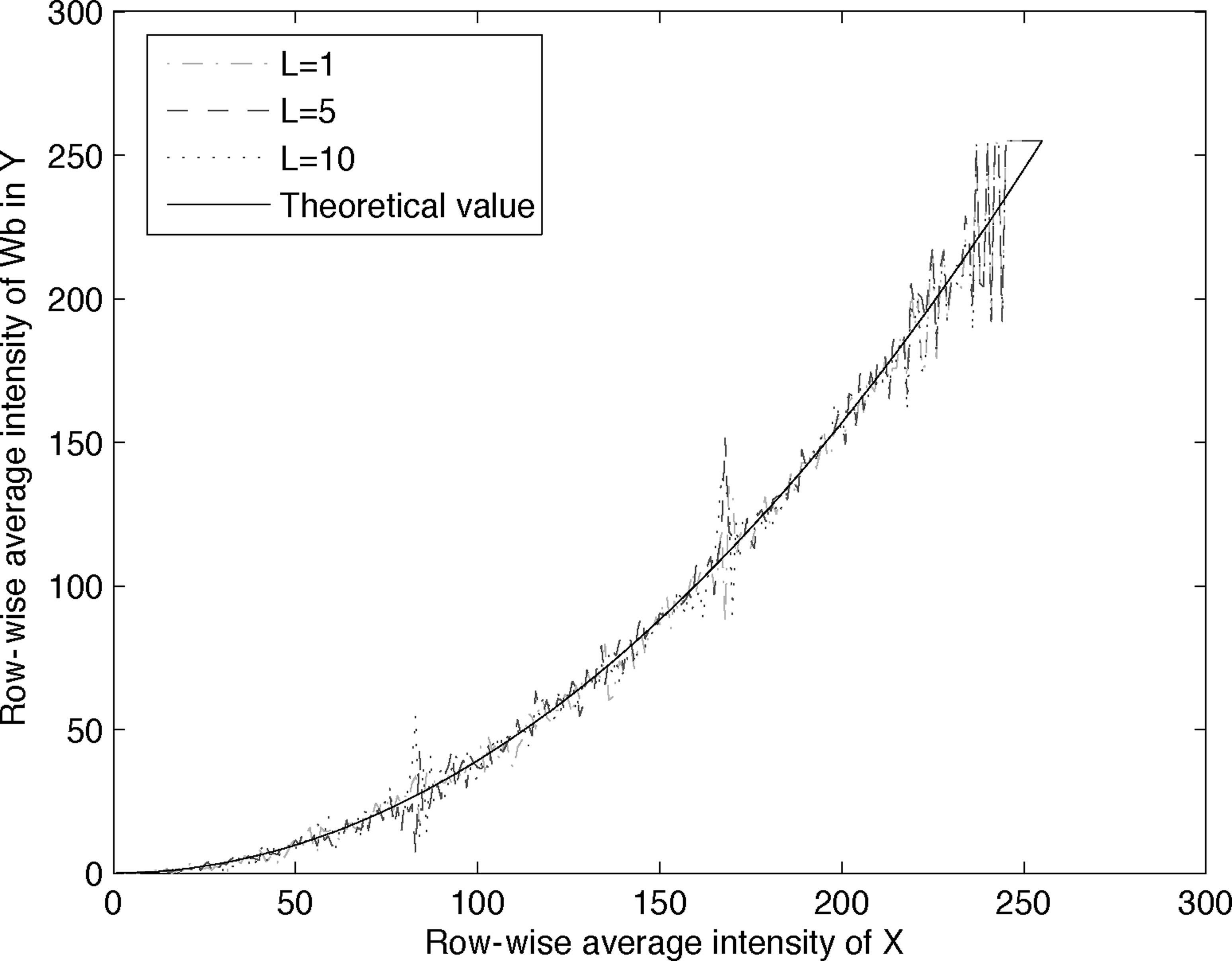
FIGURE 376.13
Row-wise average intensity of Wb in Y in Figure 13.24 vs row-wise average intensity of X in Figure 13.14 (Ramp).
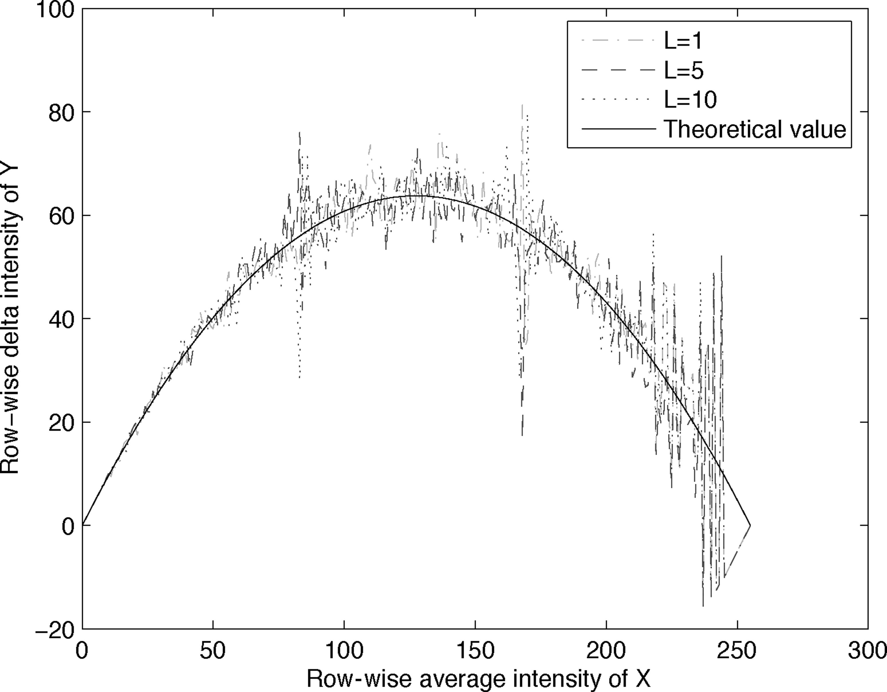
FIGURE 13.26
Row-wise Δintensity of Y in Figure 13.24 vs row-wise average intensity of X in Figure 13.14 (Ramp).

FIGURE 377.13
Contrast of Y in Figure 13.24 vs row-wise average intensity of X in Figure 13.14 (Ramp).
Comparing DHCED and DHSED, they have the same Y1. For their Y2, their pixel values are identical in Ww but different in Wb. On overlaying the corresponding Y1 and Y2, the Y of both DHCED and DHSED are identical in Ww, but DHCED has lower E[y(i, j)] in Wb than DHSED such that the black patterns of W would look darker in DHCED than in DHSED as predicted by Figure 13.29. And, the contrast of the revealed W in DHCED is higher than that in DHSED as predicted by Figure 13.30.
13.6 Summary
In this chapter, we introduce two ways to achieve steganography in halftone images, namely DHSED and DHCED. Both methods can embed a binary secret pattern into two halftone images that come from the same multitone image. When the two halftone images are overlaid, the secret pattern is revealed. DHCED can further embed a binary secret pattern into two halftone images from two different multitone images. DHSED operates by introducing different stochastic phases in the two images. DHCED operates by favoring certain conjugate values for each pixel and taking on the values only if the implied distortion is small enough. Both theoretical analysis and simulation results suggest that DHCED can give better contrast of the revealed secret pattern than DHSED.

FIGURE 13.28
Row-wise average intensity Y1 in Figure 13.4 and Y2 in Figure 13.23 vs rowwise average intensity of X in Figure 13.14 (Ramp).

FIGURE 13.29
Theoretical average local intensity of Wb in Y for DHSED and DHCED vs row-wise average intensity of X in Figure 13.14 (Ramp).

FIGURE 379.13
Theoretical contrast of Y for DHSED and DHCED vs row-wise average intensity of X in Figure 13.14 (Ramp).
Bibliography
[1] B.E. Bayers. An optimum method for two level rendition of continuous tone pictures. In Proceedings of the IEEE International Communication Conference, pages 2611–2615, 1973.
[2] R.W. Floyd and L. Steinberg. An adaptive algorithm for spatial grayscale. In Proceedings of the Society of Information Display, volume 17, pages 75–77, 1976.
[3] M.S. Fu and O.C. Au. Data hiding in halftone images by stochastic error diffusion. In Proceedings of the IEEE International Conference on Acoustics, Speech, and Signal Processing, volume 3, pages 1965–1968, May 2001.
[4] M.S. Fu and O.C. Au. Steganography in halftone images: Conjugate error diffusion. Signal Processing, 83((10):2171–2178, 2003.
[5] J.F. Jarvis, C.N. Judice, and W.H. Ninke. A survey of techniques for the display of continuous tone pictures on bilevel displays. Computer Graphics and Image Processing, 5((1):13–40, 1976.
[6] P. Moulin and R. Koetter. Data-hiding codes. In Proceedings of the IEEE, volume 93, pages 2083–2126, December 2005.